Studies on Reliability and Measurement Error of Measurements in Medicine – From Design to Statistics Explained for Medical Researchers

Introduction

Suppose you are conducting a clinical trial in healthy cross-country athletes, and the primary outcome is Achilles tendon cross-sectional area (CSA) measurement as assessed by magnetic resonance imaging (MRI).¹ Should the same rater assign the Achilles tendon CSA score to the images at baseline and at follow-up moments for each person? And can you assume that if one technician acquires the set of images of a particular person, the CSA score will be the same as when another technician would have acquired the images for the same person? Can you use the results of a reliability study conducted with an Esaote E-Scan XQ (Genoa, Italy, 0.18 T), whereas the MRI device available in your hospital is the Philips Achieva 3T MRI scanner (Best, the Netherlands)?

All these questions are reliability questions. They refer to whether specific sources of variation influence the score (also called value or result) of the individual measurement. The sources of variation described in the example above are different raters, technicians, or machines. Other examples of sources of variation include different occasions (such as moments of the day or different days) when measurements are repeated, different rater’s backgrounds, different environments, different modes of administration or different software (see Appendix 1 for an overview).²

Reliability is defined as the proportion of the total variance in the measurements, which is due to “true” differences between patients.³ The aim of a reliability study is to assess whether and to what extent an instrument is able to distinguish between situations of interest. In a clinical situation, patients are often the objects of interest to be distinguished by the instrument, but it can also be healthy individuals, caregivers, clinicians, or body structures (eg, joints or lesions), etc. When the sample of objects (eg, patients) is homogenous in the construct of interest (ie, small variation between the patients in a sample), it is more difficult to distinguish between them. The goal of a reliability study is to identify important other sources of variation: ie, those that are not of interest but can substantially influence the measurement result. In other words, the goal is to identify the sources of variation that introduce the most noise. Subsequently, such sources of variation can be minimized where possible, and the reliability study repeated to document the reduction in noise. For example, in an inter-rater reliability study, the influence of having different raters involved in the measurement is investigated. If this influence is small, the score obtained by one rater can be generalized to the score obtained by another rater. In that case, it does not matter which rater takes the measurement, because raters are exchangeable. If the influence of the source of variation (eg, raters) is large, the measurement may be improved by better standardization, or by applying restrictions to that source of variation. For example, instructions to raters could be improved (better standardization) or the same rater could measure a patient over time (number of raters restricted to 1). Another option to obtain more reliable results is to take the mean score of multiple measurements as the final score. The reliability of a measurement instrument with a continuous score can be analyzed with an intraclass correlation coefficient (ICC).

Suppose now that we use the Achilles tendon cross-sectional area (CSA) measurement as assessed by magnetic resonance imaging (MRI), and we measure a score of 54.1 mm². How sure are we that this score is indeed 54.1mm²? There is a measurement error in every measurement, even in thoroughly described measurement protocols, or seemingly simple measurement instruments. In line with the classical test theory (CTT), the aim of a study on measurement error is to investigate the precision of the score based on an additive error model. Measurement error is defined as “the systematic and random error of a patient’s score that is not attributed to true changes in the construct to be measured”.³ The measurement error refers to the precision of the numerical size of a score of a patient. It refers to how similar the scores of repeated measurements in a (single) stable patient are to each other.⁴ The measurement error of a measurement instrument with a continuous score can be analyzed with the standard error of measurement (SEM) – not to be confused with the standard error of the mean – and is expressed in the unit of measurement. The SEM of the Achilles tendon CSA measurement as assessed by MRI was shown to be 1.3 mm².¹ In 95% of cases, we can trust that a person’s score will lie in the range between the observed score plus and minus 1.96 times the SEM, ie, with a score of 54.1 mm² between 51.6 mm² and 56.6 mm².

In addition to evaluating the reliability and measurement error of a measurement instrument, other measurement properties are also important to evaluate to understand the quality of a measurement instrument, such as various forms of validity, and responsiveness.³ However, these measurement properties can be investigated in separate studies, each having other design requirements and preferred statistical methods, and are beyond the scope of this paper.

Reliability and measurement error are two closely related but distinct measurement properties that can be assessed with the same data collected.² Several designs can be chosen to assess reliability and measurement error of a measurement instrument, and each design includes one or more sources of variation. Designing such studies and certainly choosing the appropriate ICC and SEM formulas can be challenging, and choices depend on the number of sources of variation and the purpose of the measurement.

The theory for reliability that we use in this study is based on the CTT and its extension, Generalizability (G) theory. Many books and methodological papers have been written about understanding ICCs and G theory from a statistical perspective (e.g.),^5,6 which may be rather difficult to understand for many medical researchers. Moreover, often the examples used are from behavioral and social science^7,8 or education⁹ where the focus is often on the reliability of individual items that measure a construct (ie, internal consistency). In clinical measurement instruments, it is often not possible to replace specific items or variables with comparable others (for examples as can be done in a math test) or remove unreliable items altogether (for example in measurements based on one parameter obtained from an image). As studies on reliability and measurement error are important to undertake for clinical measurement instruments, we aim to explain how to design and conduct such studies in the medical field for instruments with continuous (total) scores. In this paper, we explain reliability and measurement error studies as they are performed in clinical measurements with continuous scores by listing the most frequent research questions, clarifying the resulting design choices, and the corresponding statistical formulas for ICCs and SEMs. In Section 1, we will explain the design choices. This section is based on results of a Delphi study on developing standards for assessing the quality of studies on reliability and measurement error.² In Section 2, we will introduce CTT and G theory, some specific terminology from G theory, and explain the general idea of applying Venn diagrams to visualize the design of a reliability study. In Section 3, we use the Venn diagrams to explain the requirements for data collection and the calculation of the corresponding formulas for reliability and measurement error. When results of studies on reliability and measurement error show that the measurement needs to be improved, one method to do so is by taking the average of repeated measurements, to arrive at a more reliable score on the measurement. In Section 4 on D-studies, we explain how to choose the number of repetitions. We close the paper with recommendations on reporting in Section 5.

In a reliability study, one or more potential sources of variation are investigated. In our terminology, the “rater” (r) assigns the score, the “technician” (t) acquires an image, and the “machine” (m) applies the specific technique to obtain the image (eg, MRI or positron emission tomography (PET)), often a specific brand of a machine (eg, Esaote or Philips). We use “patients” (p) to indicate the population of interest throughout this paper. We use the term “score” when we refer to the result of a measurement (either categorical or continuous) and “result” when we refer to the outcomes of the study on reliability or measurement error. In this paper, we will only focus on continuous scores, and on the parameters ICC or SEM based on variance components.

Section 1. How to Design a Study on Reliability and Measurement Error?

The basic design of a study on reliability or measurement error includes repeated measurements in stable patients. However, many choices can be made about how these measurements are actually performed, for example, which machine is used, whether the same rater performed the measurement, or whether patients received specific instructions to perform the measurement. Each of these choices leads to a different design (and a different research question). Table 1 summarizes the design choices in 7 points.² Below, we explain each of the choices.

Table 1 Choices to Be Made in the Design of a Study on Reliability or Measurement Error

In addition to these seven choices, we need also to decide upon the number of repeated measurements and the sample size of the patients. Therefore, based on simulation studies, we developed an online application to facilitate these decisions.^10,11

1: The Name of the Outcome Measurement Instrument

The name of the measurement instrument may be obvious, for example, the PROMIS physical function item bank,¹² or the Nine Hole Peg Test.¹³ In other cases, it might be less straightforward, for example in the case of an imaging technique. There, the instrument is actually a combination of the technique or machine being used (eg, ultrasound), and the parameter being assessed, such as the “Greyscale ultrasound synovial thickening (synovial hypertrophy)”, Doppler ultrasound increased blood flow (Synovial hyperemia). Another example: “basal cell carcinoma lesions measured with real-time in vivo reflectance confocal microscopy”.

2: The Version of the Outcome Measurement Instrument or Way of Operationalization of the Measurement Protocol

Instruments can appear in various forms. For example, variation occurs in the number of items (eg, in the pain observation scale Doloplus¹⁴ version 1 had 15 items, but version 2 only 10), the duration of a test (eg, the walking test has 2, 6 and 12-minute versions),¹⁵ or the language used (eg, the English¹⁶ or Dutch version¹⁷ of the SF-36 Health Survey). Other details of the measurement protocol implementation may also be relevant, for example the professional background and expertise of the raters involved, the brand and type of the machine used, the moment of the day when the measurement is conducted, etc. These details refer to known or assumed source of variation that influence the score. However, as these sources of variation are not the focus of the study, these sources are actually kept stable across the repeated measurements (eg, restricted to use only one version of the measurement protocol). Documentation of such restrictions is important because they determine the extent of generalization, ie, to which version(s) or operationalization(s) of measurement instrument the results of the study apply and to which they do not apply.

In G theory, a restricted source of variation is called a facet of stratification.⁹ If the brand of the machine is a facet of stratification, each patient is only measured by one particular brand. It is also possible that more than one element is selected from the facet of stratification, for example two types of machines. In that case, part of the patients is only measured with machine A, while another part of the patients is only measured with machine B. The results can then only be applied to these two types of machines.

3: The Construct Measured by the Measurement Instrument

The construct, also called the outcome, the concept, or the (latent) trait, refers to what is being measured. The construct should be specified for reasons of clarity. When the name of the measurement instrument is the combination of the type of machine (eg, ultra sound (US)) and the parameter that is measured (eg, “Achilles tendon CSA measurement on US imaging”)¹ the specific parameter directly refers to the construct to be measured. However, it is not immediately clear that “Doloplus-2” concerns behavioral assessment of pain,¹⁴ so this should be made explicit.

4: Measurement Property of Interest

In the introduction of this paper, we explained that reliability and measurement error are two related but distinct measurement properties that can be investigated within the same study design and the same data. Reliability focuses on whether and to what extent potential sources of variation influence the score, whereas measurement error focuses on how close the scores of repeated measurements are to each other in a stable patient.⁴ Reliability is relevant when one wants to improve the measurement instrument (eg, the measurement protocol), whereas measurement error is relevant when one is using the measurement instrument as it is.² As both measurement properties can be calculated within in the same design and data collection, we recommend to always assess both measurement properties.

5: Components of the Measurement Instrument That Will Be Repeated

A study on reliability or measurement error concerns repeated measurements in stable patients.⁴ Either the whole measurement can be repeated or only some of its components (Appendix 1).² For example, when the reliability of the Achilles tendon CSA measurement by MRI is studied, the assessment of the entire measurement instrument should be repeated (Figure 1). This means that images should be acquired twice for each patient (eg, on separate days). However, we could also be interested in the reliability of the assignment of the CSA score of static MRI images, for example by different raters. In this case, we are interested in the inter-rater reliability of the assignment of the scores of static images. In such a study design, only the final component (the assignment of the score) is repeated (Figure 2).

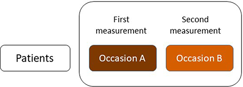Figure 1 Test–retest design of the assessment of reliability or measurement error of the entire measurement instrument.

Figure 2 Inter-rater design of the assessment of reliability or measurement error of the assignment of the score.

Note that when only the component “assignment of the score” is repeated (Figure 2), and subsequently the reliability or measurement error is calculated, the error introduced by the components that are not repeated (ie, equipment, preparation actions, collection of raw data, and data processing and storage) are not taken into account in the results of the study.

6: Specification of the Source(s) of Variation That Will Be Varied Across the Repeated Measurements

Often, one specific source of variation is varied across the repeated measurements, because you want to know whether (and to what extent) this specific source of variation influences the score. Examples of sources of variation are time or occasion (test–retest or intra-rater design), the professionals (inter-rater design), or the machines (inter-machine or inter-device design).¹⁸ This specific source of variation is then the focus of interest of the study to be varied across the repeated measurements within patients in the design. If this source of variation is found to be influential, it may be minimized through better standardization or restriction, to improve reliability of the measurement. In G theory, this source of variation is called the facet of generalization.⁹

The research question of interest has consequences for the assumptions that are made.¹⁹ For example, the aim is to evaluate intra-rater reliability, and patients are measured twice by the same rater within a time period of one week. In this case, we assume that there is no biological variation within patients, and patients are stable over this week on the construct of interest. If we find error in the scores, we interpret it as error due to the rater. With the same design, we could evaluate test–retest reliability: the patients are again measured twice by the same rater within a time period of one week. We are now interested in the influence of occasion, and in that case we assume that the rater is stable over time. If we do find error in the scores, we interpret this as error due to occasion, eg, instability over time or biological variation within patients.

It is also possible to simultaneously assess more than one source of variation in a single study. For example, both the technician who acquires the image and the rater who assigns the score can be varied across the repeated measurements within each patient (Figure 3). In this design, each patient is measured two times and receives a total of four scores.

Figure 3 Inter-technician inter-rater reliability design of the assessment of reliability of the entire measurement instrument.

The data from Figure 3 allow several different additional analyses. For example, the inter-rater reliability of the assignment of the score can be assessed with scores 1 and 2. If it turns out that this component does not introduce error in this part of the measurement, scores 1 and 4, for example, could be used to assess the inter-technician reliability.

A basic assumption is the independence of all measurements. That means that (1) the time interval between the repeated measurements is appropriate (depending on the construct to be measured and the patient population), to prevent recall bias, and to make sure that patients have not changed on the construct to be measured; (2) the measurement protocol was administered under the same condition in each measurement, meaning that, for example, no learning effects have occurred; and (3) the professional(s) who administered the measurement, or who assigned the score, did this without knowledge of scores or values of other repeated measurement(s) in the same patients.² If any of these issues are likely to occur, it could be taken into account in the study design, for example, when determining the appropriate time interval between measurements, or by introducing a familiarization session for conducting the measurement.

In the designs depicted in the Figures 1–3 we assume that all patients are measured by all technicians and raters involved in the study. There is only one measurement condition. For example, the aim is to assess the inter-rater reliability, and three raters are selected. Each patient is measured three times, once by each rater. This is called a crossed design, and “patients are crossed by rater”, written as “p × r”.⁷ However, there are also so-called nested designs when patients are not measured by all raters, ie, the rater is nested in the object of measurement (patient). For example, we could do a nested inter-rater reliability study where three pairs of raters (ie, three different measurement conditions) each measure one-third of the patients (see Figure 4). Another example is a nested intra-rater reliability study, where half of the patients is measured twice by rater A, and the other half twice by rater B. Both situations are written as “r: p” (“rater nested in patient”). These nested designs can be very efficient because the raters have to perform fewer assessments. In addition, this is also efficient from a practical point of view, because logistically this can often be better arranged. However, more complex statistics are required to take these different conditions into account. We will explain the statistics for nested designs in Appendix 2.

Figure 4 Nested inter-rater reliability design where the raters are nested in patients (for which we use the abbreviation: r: p).

Element 7: Patient Population

The reliability depends on the homogeneity or heterogeneity of the study population of the construct of interest. The selection of the study population (and thus its homogeneity) is an important design element. Therefore, the sample included in the study should be recruited from the population of interest. If the measurement instrument is usually applied to patients, healthy subjects should not be added in a study on the reliability and measurement error as this will create a more, unrealistic, heterogeneous sample.

In G theory, the study population is called object of measurement or the facet of differentiation.⁹ This refers to who or what is being measured and scored. Often in the clinical field, the object of measurement represents patients, and we use patients as the population of interest in this paper, but it can also be proxies, healthcare professionals, or body structures (eg, joints or lesions).²

Section 2. The Theory, Generalizability Theory Terminology and Introduction of Venn Diagrams

Classical Test Theory and Generalizability Theory

The theory for reliability is based on the classical test theory (CTT) and its extension, Generalizability (G) theory. CTT explains that each observed score is composed of two components: a true score and an error. In G theory, the true score is called the universe score. The true score remains unknown and can only be estimated, for example as an average over repeated measurements in a stable patient. The error in an observed score is due to the influence of all (known and unknown) sources of variation (apart from the influence of the patient, ie, the object of measurement). The error can be either systematic or random (residual error). Systematic error is the average difference in scores between the two “elements” of source of variation and is assumed to be the same for all patients. Next to this, there is residual (or random) error which varies from patient to patient.²⁰ The true score of the patients will influence the observed score (unless the measurement has poor validity). We hope that the variation in scores across patients is mainly due to variation in true scores, rather than to error that is due to these known and unknown other sources of variation. The main difference between CTT and G theory is that CTT estimates the influence of only one source of variation at a time in addition to the patient, while G theory can estimate the influence of multiple sources of the variation at the same time.

This influence of the true score or the error on the observed score is expressed by variance components. These variance components can be obtained in a repeated measurement design, for example by ANOVA or multilevel methods (see also below).^9,21

Generalizability Theory Terminology

Facets

Facets refer to the sources of variation that can influence the observed score of a measurement instrument.⁸ As explained in Section 1 there are three types of facets:

1. Facet of differentiation (also called the object of measurement). This refers to who or what is being measured, often patients (Section 1.7). We want to differentiate between the selected elements of this facet, and we ultimately score these elements.⁹ We assume that these elements remain stable regarding the construct being measured during the repeated measurements.

2. Facet of generalization. This is the potential source of variation (eg, technicians, raters, or occasions) that is being varied across the repeated measurements in stable patients (Section 1.6). We want to investigate the contribution of this facet to the variation in scores, in order to understand whether we can generalize a score obtained by one element from the facet (eg rater A) to a score obtained by another element from that facet (eg rater B).

3. Facet of stratification. This is a facet that could influence the score, but it is not the focus of the study and therefore restricted (ie, kept constant) across the measurements within a patient (Section 1.2). Suppose we want to evaluate the inter-technician reliability, and we know or assume that “brand of machine” is a source of variation that influences the score (Figure 5). As we are not specifically interested in the influence of the brand of the machine (m) in this study, we restrict it by using only one brand of machine for measuring each patient. By definition, the object of measurement (eg, the patient (p)) is nested in a facet of stratification. Often, only one element of a facet of stratification is selected, for example all patients are measured on an Esaote MRI machine. However, it could also be that some patients (Figure 5, patients 1–25) are measured by machine A, and other patients (Figure 5, patients 26–50) are measured by machine B, eg, Philips MRI machine. Still, patients are nested in machine. Results of the study cannot be automatically generalized beyond the facets of stratification, that is beyond the chosen brand(s) of machine.

Figure 5 Inter-technician reliability design where the patient (object of measurement) is crossed with technician (facet of generalization) (p x t), but nested in machine (facet of stratification) (p: m).

Selection of Elements and Recruitment of Study Participants

A facet consists of a universe of elements, eg, all potential patients, types of machines or raters in the world.⁹ Elements from the population (eg, the sample of patients or the raters) are selected to participate in the study. It depends on the specific context of use of the study which patients and professionals are recruited in the study. If the context is to investigate the potential quality of a newly developed measurement instrument in a population for which it is theoretically aimed to be applied, the sample of patients should be purposefully selected so that the distribution of patients is “flat” across the range of possible values of the instrument (ie, NOT “representative”, “Gaussian”, “random” or “convenience” sample from the target population). In other words, the extremes of the scale must be well represented in order to make statements about the full range of the scale. In such a study, a sample of well-trained professionals should be recruited to perform the measurement. If the quality of the instrument is established, and the context is to investigate how the instrument functions in routine care, the sample of patients should be representative of that population, and the recruited professionals should be representative of the population of professionals involved in routine care. Therefore, the context of the study determines the eligibility criteria. Based on these criteria, an adequate sample of patients (object of measurement), professionals (facets of generalization), and type(s) of machines (facet of stratification) are selected to be included in the study. In practice, a compromise is often necessary between ideal sampling and the availability of elements (patients, professionals, machines, etc.).

Agreement versus Consistency

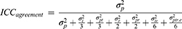
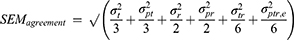
Next, we need to choose whether or not we are interested in the systematic error, that is the systematic difference of a facet of generalization. We call a difference between raters systematic if, for example, on average rater A scores 5 points higher than rater B. If we are interested in these systematic differences in the facet of generalization, we need to take it into account in the estimation of the parameters of reliability or measurement error. These parameters are then called ICC_agreement and SEM_agreement, respectively. In this case, we want to know whether we can generalize the value of a score obtained by rater A to the value of a score obtained by rater B (see Figure 6 upper panel). If we are not interested in the systematic difference, we ignore these in the parameter estimations, and we are estimating the ICC_consistency and SEM_consistency. In this situation, we are interested in whether the patients are ranked the same order in the repeated measurements (Figure 6 lower panel). The ICC_agreement is also called D-coefficient, φ-coefficient, or the absolute parameter; and for ICC_consistency the terms G-coefficient, Ερ-coefficient or the relative ICC parameter are used.

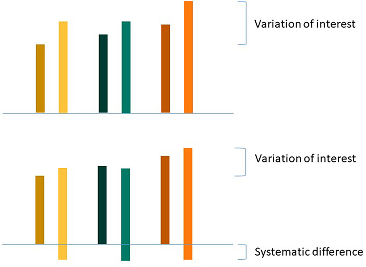Figure 6 Variation of interest for agreement parameters (upper panel) and variation of interest for consistency parameters (lower panel); patients: yellow, green, orange; raters: dark, light.

In clinical measurements, we are often interested in the absolute value of scores (agreement) rather than in a relative interpretation of scores of the patients (consistency). Therefore, we recommend in many cases in measurements in medicine to use ICC_agreement and SEM_agreement. An example of where we are interested in a relative interpretation (ie, ICC_consistency, and SEM_consistency) could be when we want to rank patients with a severity scale on a waiting list for an intervention, rather than to use the absolute scores of the severity scale. In a reliability study, two clinicians rate the severity of all patients on the same day on a 0–10 point scale. The patient with the highest urgency should have received the highest score by both clinicians, and the one with the lowest urgency should have received the lowest score by both clinicians (and so on). For this purpose of measurement, it does not matter whether one clinician is more strict and scores between, eg, 2 and 7, while the other clinician is less strict and scores between, eg, 4 and 9, as long as the ordering of the patients is the same. If the ICC_consistency is sufficient, it means that raters would order the patient in a similar way. However, it does not necessarily mean that raters would come to the same score for each patient.

To inform us on the magnitude of the systematic difference, both the agreement and consistency parameters can be estimated based on the same design, and can be compared. When the results are very close, the systematic difference is small. In Section 3, we will explain how this choice leads to different formulas for ICCs or SEMs.

Random and Fixed Facets

The ICC and SEM are constructed from variance components, which can be estimated by ANOVA or multi-level methods. In these analyses, a facet can be considered either as fixed or random. We consider it a random facet, if we want to generalize the score obtained by one element of the facet (eg by rater A) to another element (eg to rater B). In that case, we are interested in the magnitude of the systematic difference of that facet. Hence, this facets is included in the statistical model as a random component (see also Appendix 3), and the systematic variance component is estimated separately from the residual variance component.

When we are not interested in the extent of the systematic difference of a facet of generalization, this facet of generalization can be considered as fixed. Consequently, the systematic difference of the facet is removed from the calculation of the reliability parameters (ie, consistency parameters, see also Section 3) and is included as a co-variate in the statistical model to adjust the estimation of the other variance components in the model. The facet of differentiation (object of measurement) is always considered a random facet, and a facet of generalization is often considered as a random facet in medicine. A facet of stratification is always considered to be fixed, because we are not interested in the systematic difference between the chosen elements of the facet of stratification. As this facet is restricted (ie, already fixed) across repeated measurements in stable patients, it is not included in the statistical model, and we do not have to adjust for it.

When we consider the facet as random, we assume that the elements actually in our study (eg, the available raters, patients) are a random selection from the pool of possible elements (ie, population), even though raters are selected from available raters and patients are a consecutive sample. A facet is considered fixed when certain elements (from all theoretically possible elements) are purposefully selected. For example, a specific brand of machine can be selected, or the raters in a trial, where the objective is to document adequate proficiency.⁸

Venn Diagrams to Visualize the Design of a Reliability Study

Venn diagrams are used in Section 3 to derive the appropriate ICC formula corresponding to the design of the study. Here, we first explain the general idea of applying the Venn diagrams to visualize the design of a reliability study.

Assume that the observed score of a person on a measurement instrument can be depicted as a surface (Figure 7). This surface is made up of several circles. Each circle reflects a facet (including the object of measurement) – all facets together determine the observed score. Circles that partly overlap each other refer to those facets being crossed with each other. If one circle is depicted within another circle, the facet of the inner circle is nested in the other facet.

Figure 7 Venn diagrams for crossed and nested designs; diagram A = object of measurement crossed with a facet of generalization, interest in all systematic differences (agreement)(p x r); diagram B = object of measurement crossed with a facet of generalization, systematic difference ignored (consistency)(p x r); diagram C = facet of generalization nested in object of measurement (r: p); diagram D = object of measurement nested in facet of stratification (p: m), and facet of generalization nested in object of measurement (r: p). Blue surface = the variation of interest, ie, the main effect of the object of measurement; white surfaces = measurement error of interest; red surface = measurement error that will be ignored or restricted part of the measurement.

Each part of the different circles refers to the variation in score either due to the specific facet or to an interaction between two or more facets. This influence on the score is expressed in a variance component (σ²).^9,21 The influence of a facet on its own is depicted as the part of a circle that does not overlap any other circle and is called the main effect. The main effect of the facet of differentiation (object of measurement), for example the patients (), expresses the variation between the patients. Note that when this variation is large, it is a more heterogeneous population, and it is easier to distinguish between the patients. The main effect of a facet of generalization, for example that of the technician () or the rater (), expresses the systematic difference of the facet, for example between technicians or between raters, respectively. The main effect of a facet of stratification, for example the brand of machine (), cannot be assessed in the specific study, as this facet is not varied but restricted (kept constant) within the repeated measurements of a patient.

The overlapping parts represent the interaction between two or more facets (eg, or ) and are also part of the systematic error. Unknown error, coming from unknown facets that are not considered in the design, is included in the residual or random error, which also contains the interaction between all known facets. This latter interaction and the unknown error cannot be further disentangled in the current design. For example, in an inter-rater reliability design, the residual error includes all unknown errors and the interaction between the patient and the rater. In this design, the residual error is expressed as .⁵

In the diagrams A and B of Figure 7 the surface consists of three parts: the influence of the object of measurement (the main effect of the patients), which refers to the heterogeneity (true variation, ie, differences between patients in the construct being measured); the influence of the facet of generalization (main effect of the raters) which refers to the systematic difference between the elements of these facets; and finally, the interaction between the two facets patients and raters, which is depicted as the overlap between the two facets. This is the residual error (e.g. ), as it includes the unknown error in addition to this interaction.

The surface of each part of a circle is either colored (in blue or red) or white (Figure 7). The blue surfaces refer to the variation of interest, ie, what we want to differentiate. For example, the variation between patients. This is represented by the main effect of the object of measurement.

The white surfaces refer to the measurement error of interest. As there will always be some measurement error in a measurement, there will always be a white part of the surface. The measurement error always contains the residual error, which is the unknown error and the interaction between the patient and the facet(s) of generalization, represented by the overlapping part (Figure 7 diagrams A and B). When we are interested in the systematic difference of the facet of generalization (ie, agreement), we include the main effect of the facet of generalization into the measurement error of interest (Figure 7 diagram A). In Figure 7 diagrams C and D the facet of generalization (rater) is nested in the patient, and the main effect of the rater cannot be disentangled from the residual error, and it automatically is in the measurement error of interest.

Red surfaces refer to facets that will be ignored in the calculation, either because we are not interested in the systematic difference of that facet (of generalization) and have chosen to determine the consistency parameters (as in Figure 7 diagram B), or because the facet is restricted in the design of the study (not varied within the patients, ie, a facet of stratification, as in Figure 7 diagram D).

In this paper, we use an equal size for each (crossed) circle for simplicity. However, the magnitude of the variance component of a facet would determine the true size of a circle.

Section 3. How to Choose the Appropriate ICC and SEM Parameter?

Here, we discuss the specific Venn diagrams associated with a specific design and data collection scheme, where we purposefully vary none, one or two potential sources of variation across the repeated measurements within patients. We will explain various crossed designs. For related nested designs, we refer to Appendix 2.

The contribution of each facet or interaction between facets to the variation in observed scores is expressed with variance components. Information on how to calculate variance components can be found in the literature, eg, Bloch and Norman⁹ or Liljequist et al.²¹ These variance components can be obtained in a repeated measurement design, for example, by ANOVA or multilevel methods. We developed the R package “Agree” to estimate all parameters with multilevel methods.²² The advantage of a multilevel model is that this method is robust against missing data and able to deal with unbalanced designs (ie, where the number of elements of the nested facet is differently across the nests; in other words, when the sample size in each measurement condition is not the same).⁹ In addition, we developed a vignette for the Agree package, in which we explain how to calculate variance components, ICC and SEM parameters and the 95% confidence intervals for ICCs²³ (see also Appendix 3). In Appendix 4 we will show how to calculate the various variance components for crossed and nested designs in SPSS to be used in the different designs as explained below. However, SPSS ignores patients with missing data.

Below, we explain the meaning of different parts of a Venn diagram, and how to obtain the corresponding ICC and SEM. To build the Venn diagrams and the formulas, we will use a “set of rules” as formulated and explained by Brennan,⁷ Streiner and Norman,²⁴ and Bloch and Norman.⁹ We explain both agreement and consistency parameters.

Note that in different study designs, different forms of ICCs and SEMs should be applied, and different assumptions have to be made. These different studies may give different results and give specific information about the reliability and measurement error of (the different components of) the instrument under study.¹⁹

Building the ICC and SEM Formula’s

ICCs and SEMs are built from various variance components. There is no single ICC or SEM formula, but rather a whole family of formulas. The basic formula of the ICC is a ratio of the variation between the patients (the variation of interest) depicted as the blue parts, divided by the sum of the variation between patients and the measurement error of interest depicted as the white parts.^7,8 The SEM (ie, the measurement error of interest), depicted as the white parts, is calculated by taking the square root of the variance components depicted in white.²⁵

Depending on how many different facets (including the facet of differentiation, ie, the object of measurement) can be disentangled in the chosen design, a one-way, two-way or three-way model should be used to obtain the variance components. We can only disentangle a facet of generalization, when we include this in the design, and its measurement conditions are known. This means that we vary this facet across the repeated measurements in the patients and register which element of the facet of generalization is involved in which repeated measurement. For example, which rater took the first measurement, and which rater the second measurement. Please note that although in each model (ie, one-way, two-way, or three-way effects model) the variance between the patients is calculated, the magnitude of this variance component can differ between the different models. In a two- and three-way effect model, more sources of variation are recognized, and these sources are detracted from the main effect of patients.⁸

One-Way Random Effects Model: Quantification of the Measurement Error

The one-way random effects model is chosen when we want to understand whether there is any room at all to improve the measurement, given the variation between patients in our population of interest. In the most simple design of a study on reliability and measurement error, all patients have repeated measurements without using pre-defined measurement conditions for any facets of generalization.⁵ This means that each measurement is performed by any available technician, rater, etc. (Figure 8A data collection scheme). Actually, all sources of variation (eg, technician, rater, but also moment of the day, and even unknown facets) are nested in the object of measurement (patient),⁵ and we cannot disentangle any systematic difference for any facet of generalization. As we have no specific information about the influence of these potential sources, they are all part of the residual error (p,e) (Figure 8A Venn diagram), and we cannot choose between agreement or consistency parameters. This ICC is based on the one-way random effects model (Figure 8A statistical formulas), also known as ICC (1.1).⁶

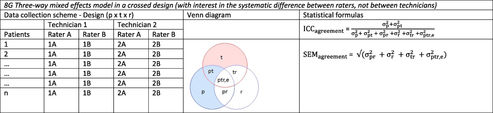
Figure 8 Continued.

Figure 8 Various one-way, two-way and three-way crossed effects model; (A) one-way random effects model; (B) two-way random effects model for agreement in crossed design; (C) two-way mixed effects model for consistency in crossed design; (D) two-way random effects model for agreement with patient nested in machine, crossed with rater; (E) three-way random effects model for agreement in a crossed design; (F) three-way mixed effects model for consistency in a crossed design; (G) three-way mixed effects model in a crossed design (with interest in the systematic difference between raters, not between technicians); n = number of included patients; A, B, C, D, E, F = refer to a specific rater; Blue surface = variation of interest, white surface = measurement error of interest, red surface = variation that will be ignored; *Unknown or no pre-defined measurement conditions were specified for any facet of generalization. Abbreviations: p, patient; p,e, residual error; r, rater; pr,e, residual error; m, machine; t, technician; pt, interaction between patient and technician; pr, interaction between patient and rater; tr, interaction between technician and rater; ptr,e, residual error; ICC, intraclass correlation coefficient, SEM, standard error of measurement; σ2, variance component.

The goal of calculating the ICC_one-way is to understand whether the score is influenced by sources of variation, other than by the variation between patients. If so (ie, a low ICC, for example, below 0.70), there may be room for improvement of the measurement instrument. The goal of calculating the SEM_one-way is to show how large the measurement error is when the measurement is applied in clinical practice or research using the measurement protocol under study, expressed in the unit of measurement of the instrument. This is extremely relevant to know when interpreting the scores of an instrument. When the measurement error is large (eg, larger than the minimal important change value), the measurement needs to be improved. In that case, a new study on reliability (using more complex designs, as will be explained below) can be conducted to understand which sources of variation influence the scores most, and whether standardizing or restricting these sources can indeed improve the measurement.

Two-Way Effects Models: Interest in One Specific Facet of Generalization

A two-way design is chosen to evaluate the influence of one additional source of variation. If one source of variation is varied over the repeated measurements within patients, using predefined measurement conditions, a two-way effects model can be used to split the influence of the specific source of variation into the systematic error and the random (residual) measurement error. The design can be crossed or nested.

In a crossed design, all patients are measured by the selected elements from that source. For example, if two raters are involved in the study, both raters measure all patients (Figure 8B data collection scheme). Both the influence (main effects) of the object of measurement () and of the facet of generalization () on the observed score can be distinguished from the residual error () (Figure 8B Venn diagram). If we want to estimate the agreement parameters, we consider the systematic difference between the raters (ie, its main effect ) also to be part of the measurement error of interest, in addition to the residual error (). Both ICC and SEM parameters are based on a two-way random effects model for agreement (Figure 8B statistical formulas), also known as ICC (2.1).⁶

Using the same design (Figure 8C data collection scheme) as we just described, we could also choose to ignore the systematic difference between the raters, and subsequently estimate the consistency parameters. The main effect of the facet of generalization is now depicted in red (see Figure 8C Venn diagram). In the statistical formulas, this main effect of the facet of generalization is ignored in the estimation of the parameters. These ICC and SEM are based on a two-way mixed effects model for consistency (Figure 8C statistical formula), also known as ICC (3.1).⁶

In a nested design, some of the patients are measured under one measurement condition (eg, one rater pair), while other patients are measured under another measurement condition (eg, another rater pair). These designs can be efficient, but are more complex, and are described in Appendix 2.

In the designs described so far, we have not yet introduced a facet of stratification. In a design with a facet of stratification, the object of measurement (patient) is nested in this facet (eg, machine) (Figure 8D Venn diagram). This occurs when, eg, some of the patients are measured with machine 1 and others are measured with machine 2 (Figure 8D data collection scheme), for example, due to practical reasons. However, the variation due to machine (ie, the main effect of machine) cannot be disentangled with the collected data, as this facet is not varied across the repeated measurements within patients but rather restricted within the patients. Therefore, this facet of stratification has only consequences for the generalization of the resulting ICC and SEM value, not for the results itself. The statistical models for the estimation of the ICC and SEM agreement and consistency parameters are therefore the same whether or not a facet of stratification is included in the design. In Figure 8D a crossed design is shown, with the estimation of the agreement parameters.

Three-Way Effects Models: Interest in Two Specific Facets of Generalization

A three-way design is chosen to evaluate the influence of two additional sources of variation. We might be interested in the influence of two different facets of generalization on the score and study these at the same time, for example technician and rater. We will explain the different models using crossed designs. The nested designs are described in Appendix 2. As the addition of a facet of stratification will not change the statistical formulas (as we just showed), we will not explain this option any further.

Crossed Design for Agreement Type of the Parameters

Suppose we are interested in the influence of both technicians and raters on scores based on images, and we involve two technicians and two raters. In this case, we want to know whether a score obtained by one technician and one rater can be generalized to a score obtained by another technician and another rater. In a crossed design, each patient is measured by two technicians, and subsequently, the two raters assign the score to each set of images, resulting in four scores for each patient (see Figures 3 and 8E data collection scheme), so we have a crossed design with two facets of generalization. Next, we want to estimate the agreement parameters, because we are interested in the systematic differences of both of the facets (Figure 8E Venn diagram). Subsequently, the main effects of the facets of generalization (ie, and ), and all interactions are included in the denominator of the ICC (and depicted by a white surface in the Venn diagram in Figure 8E), as well as in the SEM formula (Figure 8E statistical formulas).

Crossed Design for Consistency Type of the Parameters

Suppose now that we are not interested in the systematic difference of any of the facets of generalization. However, in medicine, this is more a theoretical option. In practice, we could only think of the situation of having patients on a waiting list, where the rank order of a group of patients is relevant. The way we collect our data will be the same as described above (Figures 8E and F data collection scheme). However, we ignore the main effects of the facets of generalization (i.e. + ) and also the interaction between these two ( depicted in red (Figure 8F Venn diagram) in the statistical formulas. As we are no longer interested in the influence of these facets, the interaction between this facet and the object of measurement (i.e. + ) will now be considered as part of the main effect of the object of measurement and is depicted in blue (Figure 8F Venn diagram). Subsequently, both interactions are moved from the denominator in the ICC formula to the nominator in the ICC formula for consistency and ignored in the SEM formula for consistency. Now, the measurement error consists only of the residual error (i.e., ).

Crossed Design with One Random and One Fixed Facet of Generalization

We could think of a situation in which we include two facets of generalization, while we are only interested in the systematic difference of one of the two facets of generalization. For example, the patients are recruited from two hospitals because it is impossible to recruit enough patients from a single hospital. Suppose each hospital only has one technician, but both technicians will acquire a set of images for each patient in both hospitals (Figure 8G data collection scheme). Next, two raters are involved, and each rater assigns a score based on each set of images for each patient (resulting in four scores per patient, see also Figure 3). In future clinical practice, the measurements will be conducted by the very same technician (ie, in their own hospital), but the set of images can be scored by any of the raters. In this case, we are not interested in a systematic difference between the technicians , but only in the systematic difference between the raters (Figure 8G Venn diagram). The interaction between patient and technician () is now moved from the measurement error to the variation of interest (blue), while the interaction between the two facets of generalization () is still included in the measurement error of interest (white).

Section 4. Decision (D-) Studies

So far, we focus on the reliability and measurement error of one measurement. This means that the results of ICC or SEM studies refer to the situation where only one measurement is taken when the instrument is used, for example, in research or clinical practice. However, we do need repeated measurements to estimate the parameters. One of the ways to increase the reliability if it is too low (eg, below 0.70) and decrease the measurement error if it is rather large (eg, larger than the minimal important change value) is to use repeated measurements and take the average score of multiple measurements as the final score. Examples of such measurements are blood pressure measurements (where the average of three measurements is taken), multiple items in a unidimensional scale (where the sum score is calculated as the final score), or when parts of an imaging technique is repeated (for example, when a marker is placed on an image three times, and the average of the three placements is used as a result of the measurement).²⁶

The question arises how often (part of) the measurement should be repeated to reach adequate reliability, and this can be answered in a Decision (D-) study,^8,24 applying the formulas and variance components as explained above. We can divide a variance component (eg, estimated in a design with two repeated measurements) by another number of repetitions (eg, 3), to calculate how many repetitions are needed for the ICC to be high enough (eg, above 0.70).⁸

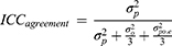
For example, we want to improve a measurement by taking the average of three occasions (eg, in a blood pressure measurement). In the formula of the ICC_agreement of an intra-rater reliability study (see Figure 8B where the facet of generalization is now “occasion” instead of “rater”), we can now divide each variance component that contains “occasion” by 3.

If we want to know the appropriate number of items in a unidimensional scale, the facet of generalization is “item”, and we can calculate which number of repeated items would lead to a sufficiently high ICC value.⁸

When we designed our study in such a way that we have three repeated measurements for the placement of the markers by the technicians , as well as two repeated measurements for the assignment of the score by the rater , we can work out which measurement strategy best optimizes the ICC: either by repeating the placement of the marker (t) or by repeating the assignment of the score (r), or even by repeating both. In the first case, all variance components containing “t” can be divided by 3; in the second case all variance components containing “r” can be divided by 2; and in the third case, the variance components are either divided by the number of t, r or t × r:

Note that the consequence of concluding about a specific measurement strategy is that future measurement should be conducted with the same measurement strategy (ie, the suggested repetitions). Issues of feasibility will, together with the results of the D-studies, lead to the most efficient choice of performing the future measurements to obtain a reliable score.

Section 5. Recommendations About Reporting on Studies of Reliability and Measurement Error

To report a study on reliability or measurement error, some guidance is available.^27,28 Based on our overview of designs of reliability studies, we emphasize that it is essential to clearly state the research question of the study, including the seven choices that are described in Section 1 of this paper and the context of use of the study (eg, whether it aims to test the potential quality of the measurement instrument or to test the applicability of the instrument in a specific population and setting). We recommend not only to estimate but also to report both reliability and measurement error. Next, we recommend to always report the ICC_agreement and SEM_agreement parameters; parameters for consistency are only relevant if assessing consistency is the specific aim of the study. Further, we strongly recommend reporting the values of all variance components, as this facilitates the comparison and pooling of studies in systematic reviews. Finally, we recommend to report the 95% confidence intervals for ICC⁶ and SEM, as this allows users to understand the precision of the ICC and SEM estimations,²³ and is needed for pooling the results. To estimate 95% confidence intervals for ICCs based on one- and two-way effects models analytical methods are available from the Agree package^22,29 (see also Appendix 3). To estimate 95% confidence intervals for three-way ICCs and SEMs bootstrap methods can be used.^30,31

Discussion

In this paper, we explained how various studies on reliability and measurement error can be designed, conducted and reported. We explained the various choices for designing such studies and showed data collection schemes, Venn diagrams and ICC and SEM formulas. Each design answers another research question. The choices to be made, as described in Section 1, can be understood as suggestions for formulating comprehensive research questions. The measurement schemes that we showed in the Figures in Section 1, and the Venn diagrams in Section 2 can be used in future studies on reliability and measurement error of outcome measurement instruments to facilitate well-considered design, analysis and reporting of these studies. In the measurement schemes, what is being repeated and what is being varied can be easily visualized to improve the understanding of readers. The Venn diagrams can help to easily build the appropriate statistical formulas for the study.

With regard to the analyses, the estimation of the variance components can be calculated in R²³ or in SPSS (Appendix 4).³² The calculation of the parameters in the various effects models, and the 95% confidence intervals of ICCs can be calculated in R.²³ Several other software programs exist for calculations of the variance components and the parameters, for example urGENOVA^7,33 or G_String.⁹

We need to point out that there is still some heterogeneity in the definitions of various key concepts between research fields (eg, medical vs social and behavioral sciences). Our definitions are based on consensus achieved within the COSMIN framework³ that we developed because consensus was lacking. Many different definitions have led to confusion about which measurement properties are relevant and which concepts they represent. The consensus-based definitions for reliability and measurement error are technical definitions. In this paper, we use conceptual definitions, which are in line with the consensus reached in the COSMIN study (Table 2).

Table 2 COSMIN Definitions and Conceptual Definitions Used in This Paper

The two measurement properties, reliability and measurement error, are relevant for different purposes. We may want to know whether we can improve the measurement instrument or measurement protocol. Therefore, we can conduct a repeated measurement study in stable patients in which we vary one or two sources that may influence the score. By looking at the variance components we get an idea which sources may be improved (by better standardizing or restricting the source). A goal could also be to study whether a score obtained by one element from a source (eg, one rater) can be generalized to another element (eg, another rater). The ICC informs as to whether such a generalization is possible (an often used cut-off value is 0.70). Yet another goal could be to evaluate how large the error is, and the extent to which we can trust an observed score. Therefore, we can estimate the standard error of measurement (ie, the measurement error of a single score), or the smallest detectable change (SDC) value (ie, 1.96 * √2 * SEM as the measurement error of a change score). These values, expressed in the unit of measurement, can be compared against meaningful other values, such as the minimal important change (MIC) value.³⁴

With regard to the sample size of reliability studies, to come to precise ICC and SEM estimation based on one-way effects models, an analytical approach can be used.³⁵ In addition, we performed simulation studies to investigate for which conditions of sample size of patients and number of repeated measurements (eg, raters) the optimal design (ie, balance between precise and efficient) to estimate the ICC and SEM can be achieved.¹¹ In these simulation studies, we restricted the analyses to select conditions for one-way and two-way effects models. Tailored recommendations can be found in the Sample Size Decision assistant for studies on reliability and measurement error.¹⁰ We are not aware of any sample size recommendations for studies using three-way effects models.

In this current paper, we focused on estimating the ICC and SEM by use of variance components. There are also other ways to arrive at the SEM estimations. One way is derived from the SD_difference, that is standard deviation of the difference of the scores on the repeated measurements, ie, with the formula SEM = SD_difference/√2, or based on the limits of agreement in a Bland and Altman plot.²⁵ Note that in these methods the systematic change between the repeated measurements (eg, systematic difference between raters) is ignored, and it equals the SEM_consistency.

Another way is derived directly from the ICC results, ie, with the formula SEM = SD * (√ 1-ICC). The standard deviation in this formula refers to the SD_pooled of the sample, that is of SD_test and SD_retest. This pooled SD ignores the systematic difference between the repeated measurements.²⁵ Note that this formula is often misused, ie, when an ICC from another population is used, for example a more heterogeneous population,²⁵ or when Cronbach’s alpha is used as the reliability parameter instead of the ICC. Cronbach’s alpha is based on a single measurement and only takes the systematic difference between the items into account.²⁵

In this paper, we focused on the design and the building of appropriate formulas within the scope of classical test theory. Modern test theory (item response theory) may also add to understanding the quality of measurement instruments consisting of a unidimensional multi-item scale and based on a reflective model. We recommend to consult a statistician or psychometrician when designing and analyzing complex studies on reliability and measurement error. Information on basic assumptions (eg, normal distribution of the measurements, equal population variances in the replicates, and equal correlation between pairs of replicates if there are more than two replicates per subject) can be found in general statistical books.

Knowing the reliability and measurement error of an outcome measurement instrument is important, as a measurement with low reliability or large measurement error introduces uncertainty in the scores obtained, and subsequently in research or clinical practice in which these instruments are applied. However, people use these imprecise scores often as the “true” score in their subsequent analyses or clinical decisions. In addition to reliable and with minimal measurement error, an outcome measurement instrument should also be valid and responsive.³

Conclusion

We hope that our suggestions for formulating comprehensive research questions, the measurement schemes as we showed in the Figures in Section 1, and the Venn diagrams in Section 3, will be used in future studies on reliability and measurement error of outcome measurement instruments to facilitate the reporting, comparison and pooling of the results of these studies in systematic reviews. We also hope that the use of Generalizability theory in biomedical research brings as much insight in measurement errors as it has done in other science areas. The knowledge of reliability of measurements and insight into the most important sources of measurement error can give clues to improve the quality of clinical measurements.

References

1. Stenroth L, Sefa S, Arokoski J, Toyras J. Does magnetic resonance imaging provide superior reliability for achilles and patellar tendon cross-sectional area measurements compared with ultrasound imaging? Ultrasound Med Biol. 2019;45(12):3186–3198. doi:10.1016/j.ultrasmedbio.2019.08.001
2. Mokkink LB, Boers M, van der Vleuten CPM, et al. COSMIN risk of bias tool to assess the quality of studies on reliability or measurement error of outcome measurement instruments: a Delphi study. BMC Med Res Methodol. 2020;20(1). doi:10.1186/s12874-020-01179-5
3. Mokkink LB, Terwee CB, Patrick DL, et al. The COSMIN study reached international consensus on taxonomy, terminology, and definitions of measurement properties for health-related patient-reported outcomes. J Clin Epidemiol. 2010;63(7):737–745. doi:10.1016/j.jclinepi.2010.02.006
4. de Vet HC, Terwee CB, Knol DL, Bouter LM. When to use agreement versus reliability measures. J Clin Epidemiol. 2006;59:1033–1039. doi:10.1016/j.jclinepi.2005.10.015
5. McGraw KO, Wong SP. Forming inferences about some intraclass correlation coefficients. Psychol Methods. 1996;1:30–46. doi:10.1037/1082-989X.1.1.30
6. Shrout PE, Fleiss JL. Intraclass correlations: uses in assessing rater reliability. Psychol Bull. 1979;86:420–428. doi:10.1037/0033-2909.86.2.420
7. Brennan RL. Generalizability theory. Statistics for Social Science and Public Policy. Springer-Verlag; 2001.
8. Shavelson RJ, Webb NM. Generalizability theory. A Primer. Vol 1. Measurement Methods for the Social Science. Sage Publishing; 1991.
9. Bloch R, Norman G. Generalizability theory for the perplexed: a practical introduction and guide: AMEE Guide No. 68. Med Teach. 2012;34(11):960–992. doi:10.3109/0142159X.2012.703791
10. Eekhout I, Mokkink LB. ICC & SEM power: sample size decision assistant for studies on reliability and measurement error; 2022. Available from: https://iriseekhout.shinyapps.io/ICCpower/.
11. Mokkink LB, HCWd V, Diemeer S, Eekhout I. Sample size recommendations for studies on reliability and measurement error: an online application based on simulation studies. Health Serv Outcomes Res Method. 2022. doi:10.1007/s10742-022-00293-9
12. Rose M, Bjorner JB, Gandek B, Bruce B, Fries JF, Ware JE. The PROMIS physical function item bank was calibrated to a standardized metric and shown to improve measurement efficiency. J Clin Epidemiol. 2014;67(5):516–526. doi:10.1016/j.jclinepi.2013.10.024
13. Fischer JS, Jak AJ, Kniker JE, Rudick RA, Cutter G. Multiple Sclerosis Functional Composite (MSFC). Administration and Scoring Manual. National Multiple Sclerosis Society; 2001.
14. Holen JC, Saltvedt I, Fayers PM, Hjermstad MJ, Loge JH, Kaasa S. Doloplus-2, a valid tool for behavioural pain assessment? BMC Geriatr. 2007;7:29. doi:10.1186/1471-2318-7-29
15. Butland RJ, Pang J, Gross ER, Woodcock AA, Geddes DM. Two-, six-, and 12-minute walking tests in respiratory disease. Br Med J. 1982;284(6329):1607–1608. doi:10.1136/bmj.284.6329.1607
16. Ware JE, Sherbourne CD. The MOS 36-item short-form health survey (SF-36). I. Conceptual framework and item selection. Med Care. 1992;30(6):473–483. doi:10.1097/00005650-199206000-00002
17. Aaronson NK, Muller M, Cohen PD, et al. Translation, validation, and norming of the Dutch language version of the SF-36 Health Survey in community and chronic disease populations. J Clin Epidemiol. 1998;51(11):1055–1068. doi:10.1016/s0895-4356(98)00097-3
18. Gellhorn AC, Carlson MJ. Inter-rater, intra-rater, and inter-machine reliability of quantitative ultrasound measurements of the patellar tendon. Ultrasound Med Biol. 2013;39(5):791–796. doi:10.1016/j.ultrasmedbio.2012.12.001
19. Koo TK, Li MY. A guideline of selecting and reporting intraclass correlation coefficients for reliability research. J Chiropr Med. 2016;15(2):155–163. doi:10.1016/j.jcm.2016.02.012
20. White E, Armstrong BK, Saracci R. Principles of Exposure Measurement in Epidemiology. Collecting, Evaluating, and Improving Measures of Disease Risk Factors. Oxford University Press; 2008.
21. Liljequist D, Elfving B, Skavberg Roaldsen K. Intraclass correlation - A discussion and demonstration of basic features. PLoS One. 2019;14(7):e0219854. doi:10.1371/journal.pone.0219854
22. Eekhout I. Agree: agreement and reliability between multiple raters. R package version 0.1.8. Available from: https://github.com/iriseekhout/Agree/.
23. Eekhout I, Mokkink LB. Estimating ICCs and SEMs with multilevel models. Available from: https://www.iriseekhout.com/r/agree/.
24. Streiner DL, Norman G. Health measurement scales. In: A Practical Guide to Their Development and Use.
25. de Vet HC, Terwee CB, Mokkink L, Knol DL. Measurement in Medicine. Practical Guides to Biostatistics and Epidemiology. Cambridge University Press; 2011.
26. Skeie EJ, Borge JA, Leboeuf-Yde C, Bolton J, Wedderkopp N. Reliability of diagnostic ultrasound in measuring the multifidus muscle. Chiropr Man Therap. 2015;23:15. doi:10.1186/s12998-015-0059-6
27. Kottner J, Audige L, Brorson S, et al. Guidelines for Reporting Reliability and Agreement Studies (GRRAS) were proposed. J Clin Epidemiol. 2011;64(1):96–106. doi:10.1016/j.jclinepi.2010.03.002
28. Gagnier JJ, Lai J, Mokkink LB, Terwee CB. COSMIN reporting guideline for studies on measurement properties of patient-reported outcome measures. Qual Life Res. 2021;30:2197–2218. doi:10.1007/s11136-021-02822-4
29. Demetrashvili N, Wit EC, van den Heuvel ER. Confidence intervals for intraclass correlation coefficients in variance components models. Stat Methods Med Res. 2016;25(5):2359–2376. doi:10.1177/0962280214522787
30. Efron B. Better bootstrap confidence intervals. J Am Stat Assoc. 1987;82(397):171–185. doi:10.1080/01621459.1987.10478410
31. Loy A, Korobova J. Bootstrapping clustered data in R using lmeresampler. arXiv. 2021;20:54.
32. de Vet HCW. Guide for the calculation of ICC in SPSS. Available from: http://www.clinimetrics.nl/images/upload/files/Chapter%205/chapter%205_5_Calculation%20of%20ICC%20in%20SPSS.pdf.
33. Brennan RL. urGENOVA. University of Iowa; 2021. Available from: https://education.uiowa.edu/research-centers/center-advanced-studies-measurement-and-assessment/computer-programs.
34. Terwee CB, Peipert JD, Chapman R, et al. Minimal important change (MIC): a conceptual clarification and systematic review of MIC estimates of PROMIS measures. Qual Life Res. 2021;30(10):2729–2754. doi:10.1007/s11136-021-02925-y
35. Zou GY. Sample size formulas for estimating intraclass correlation coefficients with precision and assurance. Stat Med. 2012;31:3972–3981. doi:10.1002/sim.5466
© 2023 The Author(s). This work is published and licensed by Dove Medical Press Limited. The
full terms of this license are available at https://www.dovepress.com/terms
and incorporate the Creative Commons Attribution
- Non Commercial (unported, 3.0) License.
By accessing the work you hereby accept the Terms. Non-commercial uses of the work are permitted
without any further permission from Dove Medical Press Limited, provided the work is properly
attributed. For permission for commercial use of this work, please see paragraphs 4.2 and 5 of our Terms.
Recommended articles
Assessing the Smallest Detectable Change of the Kessler Psychological Distress Scale Score in an Adult Population in Japan
Uchida H, Kuroiwa C, Ohki S, Takahashi K, Tsuchiya K, Kikuchi S, Hirao K
Psychology Research and Behavior Management 2023, 16:2647-2654
Published Date: 13 July 2023
Development and Validation the Uterine Fibroid Symptom and Quality of Life Short-Form: Integrating Classical and Modern Test Theory
Zhang Y, Xu W, Nie Y, Zhang J, Chen D, He C, Xu F, Bai J, Shi Q
Patient Preference and Adherence 2026, 20:594260
Published Date: 27 May 2026