The Potential of a CT-Based Machine Learning Radiomics Analysis to Differentiate Brucella and Pyogenic Spondylitis

Introduction

Spinal infections encompass a range of diseases caused by various factors, with an estimated incidence rate ranging from 0.4 to 7.2 cases per 100,000 individuals per year.^1,2 Pyogenic spondylitis (PS) is a frequently encountered condition with an acute or subacute onset in the emergency department. It has been observed to have an increasing incidence rate and is often initially misdiagnosed by healthcare professionals.^3,4 Brucella spondylitis (BS) is a common manifestation in the osteoarticular system among individuals with human Brucellosis. It occurs as a result of infections caused by different species of Brucella, and it continues to pose a significant global public health concern.^5,6 BS has been found to have a high prevalence in developing areas and countries.⁷ To diagnose spinal infections, a thorough medical history and physical examination should be conducted to identify possible risk factors for infection. Common clinical manifestations include non-specific back pain, fever, and neurological symptoms caused by compression of the spinal cord and/or nerve roots.^8,9 Fever is a common symptom but may not always be present. Approximately 50% of patients with pyogenic spine infections and even higher percentages in fungal, mycobacterial, and Brucella infections may be afebrile.¹⁰ Palpation may reveal paravertebral muscle spasm, and marked tenderness with percussion over the infected spinal segment is a consistent finding in 75% to 95% of cases. Early diagnosis of spinal infections can be challenging due to the non-specificity of symptoms and signs, leading to delayed identification that can take weeks or months.¹¹ Hence, it is vital to maintain a high level of awareness and clinical suspicion. Factors like geographic location and occupational history should be highlighted during the patient’s clinical evaluation to increase suspicion specifically for brucellosis. These include working in a slaughterhouse or meat-packing environment, recent travel to endemic regions, consuming undercooked meat or unpasteurized dairy products, engaging in hunting activities involving certain animals, assisting animals during childbirth, and working in a laboratory handling Brucella specimen.¹²

Notably, both PS and BS are among the diseases caused by bacterial infections. Initial laboratory testing should include inflammatory markers such as WBC, ESR, and CRP. They are inflammatory markers that are commonly used to help in diagnosing spinal infections. Elevated ESR is observed in 75% of cases, while an elevated CRP has a higher sensitivity of 98%.^11,13,14 WBC, on the other hand, is less reliable and can be within the normal range in up to 55% of patients with spinal infections.¹⁴ Serology screening for spinal infections typically includes agglutination tests like the plate agglutination test (PAT; tiger red plate agglutination test (RBPT; and serum (tube) agglutination test (SAT; which rely on the reactivity of antibodies against smooth lipopolysaccharide (LPS).¹⁵ Isolation of germ and/or histopathology examination of the bone, marrow and/or tissue from the surgical area of patients are the gold standard. Blood culture is the first test in the microbiologic diagnosis of Pyogenic spondylitis, and Yee et al reported the true positive rate 53.4% (31/58).¹⁶ Mangalgi et al reported an overall blood culture true positivity of 24.8%, 43.1%, and 34.9% by conventional, liquid culture, and clot culture techniques, respectively, for Brucella.¹⁷ In a study conducted on 136 patients with Pyogenic spondylitis, the reported true positive rate of tissue culture using biopsy samples was 39.7% (29/73).¹⁸ Furthermore, the high laboratory requirements for the aforementioned culturing methods cannot be met in most endemic areas due to underdeveloped economies, posing a challenge for differential diagnosis.¹⁹ Thus, it is still highly challenging to differentiate these two diseases clinically. It remains a significant hurdle.²⁰ Previous studies primarily concentrated on analyzing radiological signs.^8,21–23 Spinal infections can cause damage to the structures of the spine, including the vertebral bodies and intervertebral discs, leading to increased spinal instability. Computed tomography (CT) can clearly depict the morphological erosion and vertebral destruction.²⁴ Liu et al found that vertebral body destruction was more extensive in the PS group compared to the BS group (35.8% vs 12.5%, with a positive predictive value of 63.16%).²⁵ However, radiological findings on images can be subject to interpretation, leading to bias in interpreting similar radiological signs.²⁶ Moreover, the lesions on both exhibit quite similar characteristics, including adjacent vertebral bodies with destruction of the intervertebral disc and involvement of the paravertebral soft tissues, resulting in cold abscess formation. Consequently, it can be challenging to differentiate between BS and PS based solely on CT images at times.

It is necessary to explore innovative, rapid, and objective approaches that consider various factors to examine intricate and subtle connections among clinical and radiological risk factors and their associated outcomes. Radiomics is an emerging technique that involves the objective and quantitative characterization of lesions by quantifying imaging through the utilization of high-dimensional imaging features.²⁷ This would shift subjective signs to objective features.²⁸ The potential of radiomic features to predict cancer genetics and treatment outcomes has recently garnered significant attention.²⁹ They offer substantial promise for personalized medicine. However, there is an expected significant increase in the quantity of relevant information that requires processing beyond the capacity of current analytical approaches. Furthermore, machine learning (ML) methodologies have the potential to alleviate some of these limitations. Machine learning algorithms are emerging as powerful methods for detecting intricate underlying patterns from massive amounts of data, particularly when confronted with classification tasks, which are common challenges in the medical field.^30,31 Risk prediction entails employing computer algorithms to analyze vast datasets that comprise numerous multidimensional variables. By identifying intricate, high-dimensional, and nonlinear relationships among different clinical features, one can generate outcome predictions based on data analysis.^32–35 This will provide a new approach that improves the accuracy of diagnosis and enables timely identification of patients at risk of PS or BS, which can lead to improved outcomes and mitigate burdens and costs. Early diagnosis of patients suspected of having PS or BS using innovative non-invasive measures can reduce the need for surgery and lower the overall surgical rate.

However, we have not found any previous research that applies machine learning algorithms to diagnose spine infectious diseases through analysis of radiomics. Therefore, we developed multiple machine learning models and visualized black-box interpretations of radiomics features. The goal was to provide guidance for the clinical and radiological screening of patients with PS or BS, aiding in personalized decision-making.

Methods

Ethics Committee board of Xinjiang Medical University Affiliated First Hospital (K202309-15) gave approval to this research, which involved a retrospective analysis. Due to the retrospective study design and de-identification during the process of data collection, individual agreements and written informed consent were considered unnecessary and were therefore waived.

Patients

We retrospectively searched patients diagnosed as PS or BS from the spine surgery department from January 2017 to January 2022. The diagnosis of these patients took clinical presentations, laboratory and radiology findings into consideration. The study’s inclusion criteria were established as follows: (1) patients of or above the age of 18 years; (2) initial CT examination showed morphological changes including bony sequestrum, posterior vertebral arch involvement, spinal epiduritis, paravertebral abscess, psoas abscess, vertebral body osteolysis, vertebral compaction, spinal cord compression, nerve root compression, vertebral destruction, disc space narrowing, osteosclerosis around erosions, spondylodiscitis, paraspinal abscess, etc.; (3) clinical manifestations include fever, sweating, loss of appetite, fatigue, weight loss, spinal tenderness, paravertebral tenderness, and neurological deficits such as radiculopathy, weakness or paralysis, paresthesia, etc.; (4) raised inflammation indicators (erythrocyte sedimentation rate, C-reactive protein and white blood cell count). (5) positive bacterial culture of a biopsy specimen or positive blood culture for PS; BS were evaluated by blood or bacterial culture positivity of biopsy specimens from the affected region.¹⁰ Serum agglutination test (SAT) exhibiting a titer of ≥1/160 or histological granulomatous tissue finding were also used to diagnose BS.³⁶

The participants were excluded if they met any of the exclusion criteria, which were as follows: (1) previously infected with tuberculosis fungi, viral, parasitic infections or other types of infections that were not specified or confirmed by laboratory testing; (2) the presence of lumbosacral lesions caused by metastasis, multiple myeloma, spine deformity, bone fracture, spondylolisthesis etc.; (3) displayed a poor health status such as uncontrolled diabetes, chronic renal failure, chronic obstructive pulmonary disease, multiple-organ dysfunction syndromes (MODS) etc.; (4) history of previous spinal surgery.

In our research, following the aforementioned both inclusion criteria and exclusion criteria, a total of 138 patients were enrolled. Then, we randomly split whole cohort into training group (n = 97) and testing group (internal validation set) (n = 41) with ratio of 7:3 for further model construction and validation using function from scikit-learn library (https://scikit-learn.org/).

Patients Data Collection

The retrospectively retrieved materials include demographic and imaging data. Demographic information include age, gender, the body mass index (BMI). The imaging data used in our study consisted of CT images without contrast in Digital Imaging and Communications in Medicine (DICOM) format, which were obtained prior to surgery, which included a series of slices.

CT Acquisition

The CT scan was conducted utilizing a GE VCT 64-slice scanner (GE Medical Systems Milwaukie, USA). To achieve the desired results, a tube voltage of 120-kV was set, and the tube current was automatically adjusted. The rotation speed was set at 0.6 seconds to obtain an average slice thickness of 2.5 mm for all helical mode CT scans. The Picture archiving and communication system (PACS) was employed to obtain images via the use of the Digital Imaging and Communications in Medicine (DICOM) technology.

Extracting Radiomic Features Through Image Segmentation and Pre-Processing

To perform image segmentation and lesion identification, two experienced radiologists, M.M. and W.S., with 5 and 10 years of experience in spine imaging, independently manually delineated the lesion boundaries slice by slice. No specific thresholds were applied during the delineation process. The delineation included both bony structures and soft tissue lesions when evident. Any disagreements in the delineation of lesions were resolved through consensus. We choose to process multiple ROIs within a single case by averaging the radiomics feature values.³⁷ This was done using the open-source 3D Slicer 4.10.1 platform (https://www.slicer.org/); individually segmenting each slice. They followed the edges of the lesions and outlined all identified lesions, including multifocal or multicentric cases. Image pre-processing was done with registration and resampling to achieve a uniform pixel dimension of 1.0 x 1.0×1.0 mm3 via linear and nearest-neighbor interpolation for CT images and segmentation images, respectively.³⁸ Additionally, normalization was carried out by setting parameters normalize Scale to 100, normalize to true and binWidth to 25.

For radiomic feature extraction, the Pyradiomics package³⁹ in Python v.3.9 was utilized, extracting a total of 1535 features consisting of original and filtered features. The original features included shape-based, first-order statistical, and texture features such as gray level co-occurrence matrix (GLCM; gray-level size zone matrix, gray level run length matrix (GLRLM; neighboring gray tone difference matrix features, and gray-level dependence matrix features. Notably, the filtered features are obtained through feature transformation to the original image using wavelet, square, square root, local binary pattern 2D, Laplacian Gaussian, logarithm, exponential, and gradient.

Feature Selection and Radiomics Score Building

As described above, features consist of clinical and radiomics feature. As for the former (clinical features), we adopted using univariate logistic regression analysis. Then, multivariate analysis was performed based on the result. High dimensional feature space of image was obtained. However, the inclusion of all these features will increase the complexity of and multicollinearity of classifier and this would occur the risk of overfitting that would affect the discrimination performance of the model.⁴⁰ In our study, we aimed to select features with stable and reliable manual segmentations for further analysis. To determine this, we assessed the agreement or consistency of manual segmentations performed by different annotators using the intraclass correlation coefficient (ICC). By selecting features with a high ICC agreement, we aimed to include those that had consistent and reliable delineations of the regions of interest. This approach minimized potential variability introduced by different interpretations or delineations, ensuring the reliability of the selected features for further analysis. We only included features in our analysis that exhibited a high level of stability and suitability for segmentation based on their ICC agreement of ≥0.80. This threshold ensured that the selected features had consistent and reliable manual segmentations, making them suitable for subsequent analysis.⁴¹ Subsequently, we performed a univariate analysis to assess the screening potential of each feature. We performed t-tests for variables that followed a normal distribution and used the Mann–Whitney U-test for variables that did not follow a normal distribution. Only features with a significance level of P < 0.01 in the univariate analysis were selected for further investigation.⁴¹ To address redundancy among the features, we performed a Spearman correlation analysis and removed pairs of features with a correlation coefficient of 0.85 or higher.⁴² Both related features were eliminated from the analysis. Lastly, we employed the least absolute shrinkage and selection operator (LASSO) to identify the most relevant features while simultaneously penalizing the coefficients of unimportant features to zero. We achieved this by employing ten cross-validations and a maximum of 1,000 iterations. This technique helped us select the significant features with non-zero coefficients that were used subsequently to build our predictive model.⁴³ Radiomic scores were built by means of weighted coefficients in a linear formula.

Model Construction and Optimization

Considering the classification problem at hand, we employed a total of nine distinct machine learning models: support vector machine (SVM); logistic regression (LR); random forest (RF); extreme gradient boosting (XGBoost) classifier, light gradient boosting (LGBoost) classifier, decision tree (DT); linear discriminant analysis (LDA); k-nearest neighbor classifier (KNN); and Gaussian naive Bayes classifiers (GNB). These models were utilized to develop a predictive model based on selected features, as depicted in Figure 1, which was constructed using the training set. LR is still one of the most extensively used method in data mining.⁴⁴ DT, as nonparametric model, take no predefined special assumptions, showed great prediction ability in clinical classification task.⁴⁵ RF is a tree-based ensemble method using bagging techniques to generate a more accurate result.⁴⁶ XGBoost and LGBoost are also ensembled tree-based algorithms achieved by a procedure called boosting.⁴⁷ SVM has been reported with remarkable performance in image classification, which is realized by consuming multiple-support vectors in its intrinsic structure.^48,49

Figure 1 Workflow of this study. Abbreviations: ROI, region of interests; LASSO, least absolute shrinkage and selection operator.

Machine learning algorithms consist of many parameters. Yet, different combination of parameters will incur different prediction performance. Thus, it is necessary to carry out hyperparameters tuning.⁵⁰ We adopted grid search tuning pattern. Furthermore, we noticed conventional cross-validation (CV) might suffer data leakage risk in tuning process.⁵¹ Consequently, it is viewed as best better option using nested-resampling cross-validation techniques where the evaluation process (cv = 5) will separate from tuning procedure (cv = 4). The above-mentioned process was implemented by scikit-learn package (Version 0.23.0, https://scikit-learn.org/stable/) with Python.

Model Performance Evaluation

For each of the models, receiver operating characteristic (ROC) curves were created to gauge the discriminative capacity. We also computed area under the curve (AUC), specificity, and sensitivity to assess the models’ discriminatory potential. The calibration plot was utilized to compare predicted versus observed values for individual cases. Additionally, a decision curve analysis (DCA) was executed to appraise the clinical efficacy of diverse radiomics models.

Model Interpretation and Feature Importance

Interpreting machine learning models and identifying the essential features can be challenging since the algorithm’s accurate prediction mechanisms are often perceived as inscrutable (“black box” models). To mitigate this issue, we incorporated the permutation feature importance (PFI); local interpretable model-agnostic explanations (LIME); and Shapley additive explanation (SHAP) value methods in our study. This innovative approach aims to provide greater transparency and aid in deciphering how the algorithm makes its predictions for a particular cohort of patients. PFI, also known as Mean Decrease Accuracy (MDA); is revealing the dependence of model on specific feature.⁵² LIME learns a surrogate local model which is closer to original model, then display the weighted component of given model.⁵³ SHAP uses additive feature attribution methods and game theory of Shapley values to calculate the importance of feature. These approaches can explain various black-box ML models.⁵⁴

Statistical Analysis

We used descriptive measures between two groups (PS and BS), where continuous variables belonging to normal distributions used t-test are shown as the means ± standard deviations (SDs). To test variables that did not follow a normal distribution, we conducted a Mann–Whitney U-test. For categorical variables, we used the Chi-squared or Fisher’s exact tests, depending on the expected cell count. Variables with P values less than 0.05 were considered significant in their impact on the patient outcomes. All statistical analyses were performed using the R software (version 4.2.2; http://www.r-project.org).

Results

Clinical Characteristics

The patient features of two groups are shown in Table 1. A total of 138 cases were enrolled in this study, and all of them underwent surgical intervention.

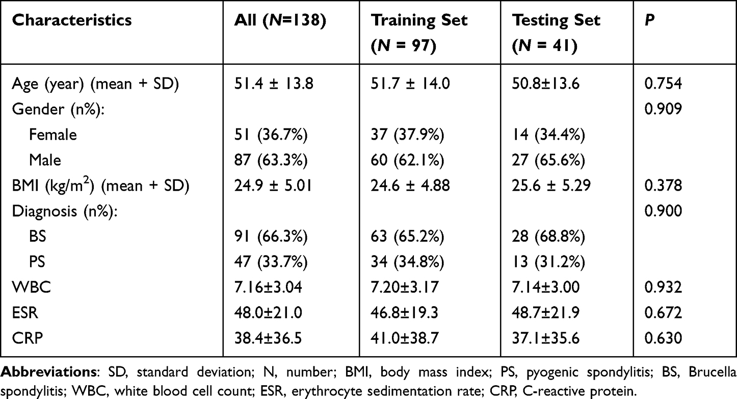Table 1 Characteristics at Baseline Between Training Set and Testing Set

Feature Selection

This study employed both univariate and multivariate logistic regression to examine the clinical characteristics of the subjects. From a total of 1535 features, we selected 956 features that demonstrated high stability and reliability, with an intraclass correlation coefficient (ICC) greater than 0.80. Feature selection was conducted using the univariate analysis method, resulting in 494 features selected. After eliminating redundant features via applying Spearman correlation analysis, we identified 62 relevant features. Lastly, for optimal feature selection, we utilized the LASSO algorithm, which identified 15 features as most effective, as illustrated in Figure 2. Furthermore, we compared the final selected features between PS and BS patients (Figure 3B) and it showed that there is no obvious collinearity existing among them (Figure 3A).

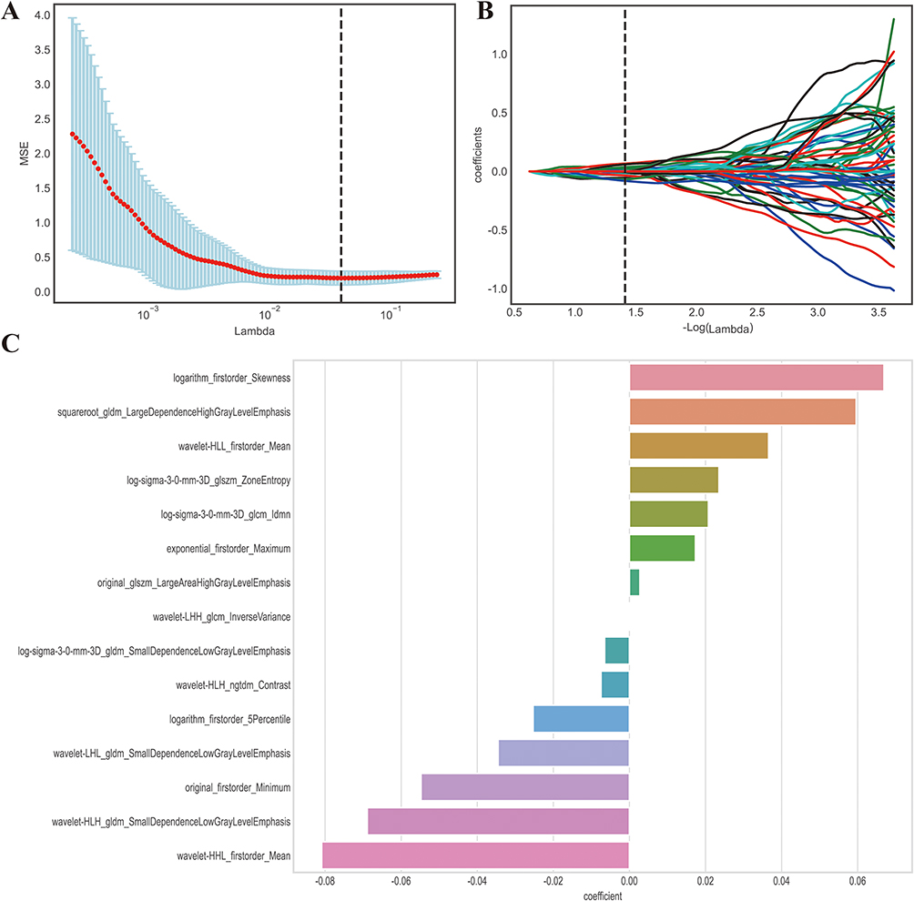Figure 2 LASSO algorithm employed for radiomics feature selection. (A) The MSE (mean square error) path represents the performance of the least absolute shrinkage and selection operator (LASSO) model at different values of the regularization parameter (lambda) utilizing 20-fold cross-validation. The lambda value (vertical dash line) that yields the lowest MSE is selected as the optimal amount of penalization. (B) LASSO coefficient profiles of the radiomics features. The coefficient profiles demonstrate the magnitude of the regression coefficients for each feature as the lambda value increases. Features with non-zero coefficients are considered selected by the LASSO model. (C) Coefficient for the 16 selected features. This component presents the magnitude of the regression coefficients for the 16 features selected by the LASSO model. The best lambda value is 0.0387, − log (lambda) is 1.412. Lambda represents the strength of the regularization penalty applied to the regression coefficients in LASSO. Vertical dash line is the best parameters (lambda) selected by LASSO cross-validation.

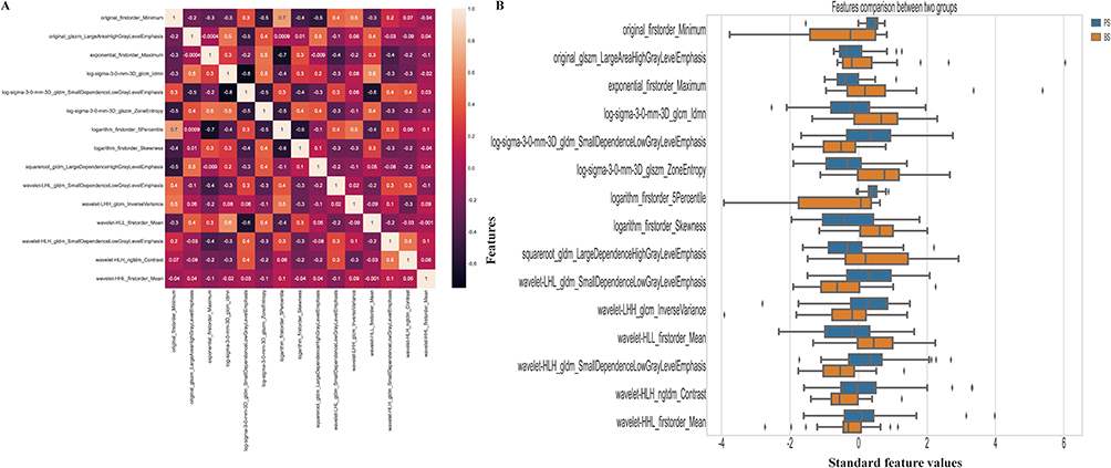Figure 3 Correlation analysis (A) and Comparison (B) of the selected features. (A) The correlation analysis heatmap of selected radiomics features. The heatmap visualizes the correlation coefficients between the selected features. Each cell in the heatmap represents the strength and direction of the correlation, with color indicating the magnitude. This analysis helps assess the relationships and potential multicollinearity among the selected features; (B) The horizontal bar plot displays a comparison of the selected radiomics features between two groups, using their standardized values. The x-axis represents the standardized values, while the y-axis displays the names of the selected features. The plot provides a visual comparison of the magnitudes of the selected features between the two groups. This information can help identify features that show significant differences between the groups.

Parameter Optimization

We compared several performance metrics for each algorithm with nested and non-nested resampling strategies respectively. The results of this analysis are presented in Figure 4, which provides a comprehensive overview of the performance of each algorithm under the different resampling strategies. The results indicate that non-nested cross-validation produces more favorable outcomes when assessing the model’s performance, potentially leading to overperformance bias. Consequently, we employed the nested cross-validation with grid-search method to fine-tune the hyperparameters of each classification algorithm.

Figure 4 Comparison of nest and non-nested cross-validation. (A) Accuracy of each classifier with and without nested cross-validation. The x-axis displays the names of the classifiers, while the y-axis represents the corresponding accuracy values achieved using both nested and non-nested cross-validation; (B) Precision of each classifier with and without nested cross-validation. The x-axis indicates the names of the classifiers, and the y-axis shows the precision values obtained using both nested and non-nested cross-validation; (C) F1 score of each classifier with and without nested cross-validation. The x-axis represents the classifier names, while the y-axis depicts the F1 score values obtained using both nested and non-nested cross-validation; (D) Recall of each classifier with and without nested cross-validation. The x-axis displays the names of the classifiers, and the y-axis shows the recall values achieved using both nested and non-nested cross-validation. Abbreviations: RF, Random Forest; XGB, Extreme Gradient Boosting; LGB, LightGBM; LDA, Linear Discriminant Analysis; LR, Logistic Regression; SVC, Support Vector Classifier; KNN, k-Nearest Neighbors; NB, Naive Bayes; DT, Decision Tree.

Classification Ability and Model Selection

In the training set, the AUC of the SVM, LR, XGBoost classifier, RF, LGBoost classifier, DT, LD, KNN, GNB classifiers were 0.93, 0.92, 1.00, 1.00,0.95, 1.00, 0.91, 0.91 and 0.93, respectively. Accordingly, in the testing set, the AUC of these seven classifiers were 0.80, 0.83, 0.84, 0.80, 0.82,0.57, 0.83, 0.87 and 0.88, respectively. The performance metrics of Recall, Brier loss, Log loss, and F1-scores consistently demonstrated that KNN outperformed other classifiers in accurately distinguishing PS from BS. Table 2 provides comprehensive details on the assessment indicators, while Figure 5 illustrates the ROC curves drawn from the classifiers employed. The calibration plot graphically demonstrates good concordance between the observed and evaluated data points, as evident from Figure 6A and B. Moreover, based on the decision curves of the five radiomic models as noticeable in Figure 6C and D, all models accurately outperformed the “treat-all-patients” and “treat-none” measures in predicting early PS. Therefore, KNN was selected for further interpretation in this study.

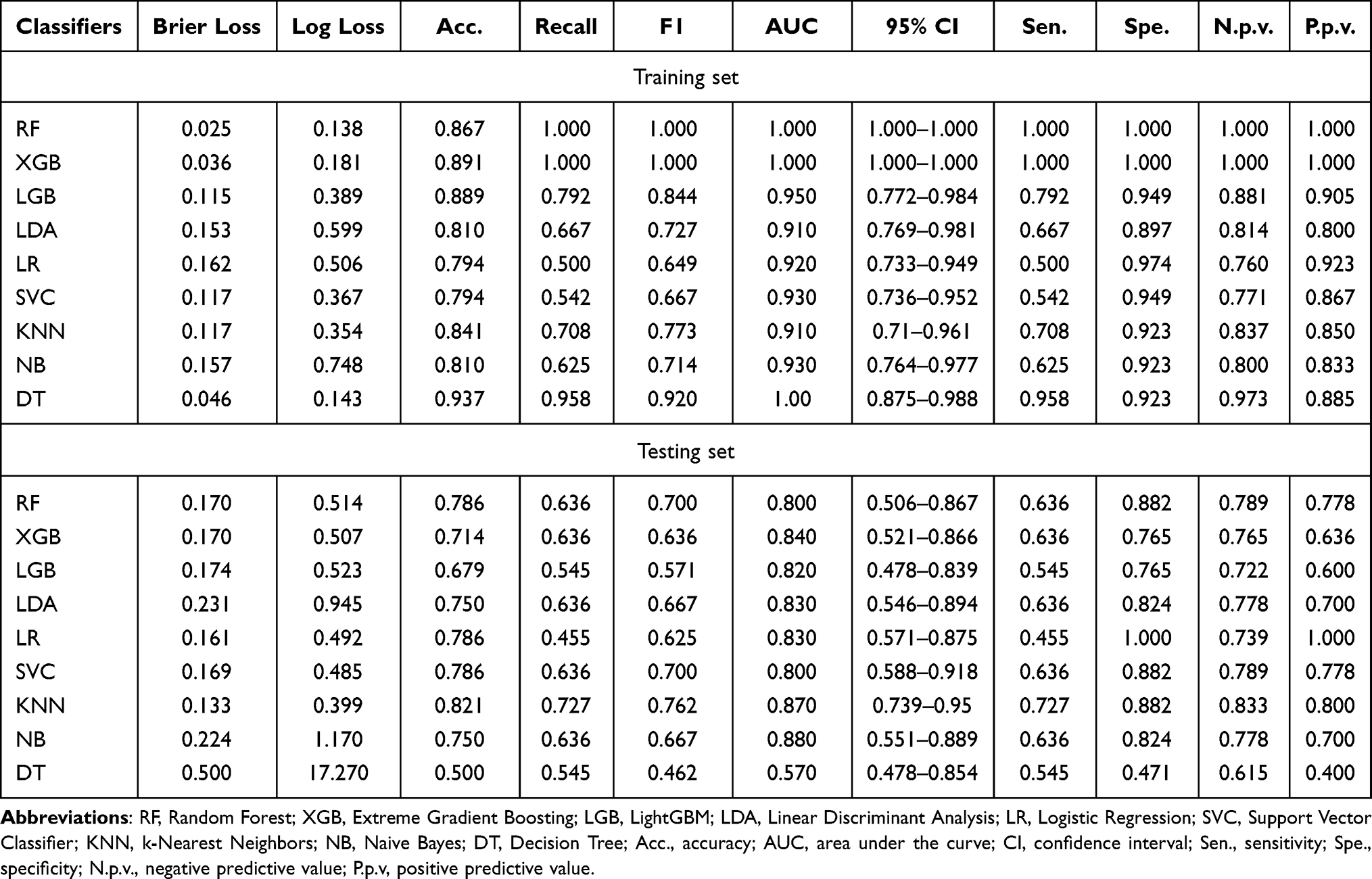Table 2 Diagnostic Performance of Each Model in the Training and Test Sets

Figure 5 The receiver operating characteristic curves (ROC) of the training set (A) and testing set (B). The receiver operating characteristic curve illustrates the tradeoff between the model’s sensitivity and its false positive rate, considering various anticipated probabilities of future Brucella spondylitis (BS). The area under this curve indicates the model’s predictive capability for estimating the probability of BS. A value of 0.5 represents a random estimator, while a perfect model would yield a value of 1.0. Abbreviations: RF, Random Forest; XGB, Extreme Gradient Boosting; LGB, LightGBM; LDA, Linear Discriminant Analysis; LR, Logistic Regression; SVC, Support Vector Classifier; KNN, k-Nearest Neighbors; NB, Naive Bayes; DT Decision Tree.

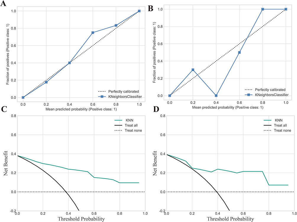Figure 6 Shows calibration curves and decision curve analysis (DCA) for the model’s performance evaluation. (A) The calibration curve for the training set; (B) The calibration curve for the testing set; (C) DCA curve for the training set; (D) DCA curve for the testing set. Calibration curves were employed to gauge the congruity between the observed and predicted diagnostic categories. Decision curve analysis (DCA) aids in appraising the model’s performance by examining the net benefit derived from employing the model at various threshold probabilities. It evaluates the balance between the sensitivity and specificity of the model and offers valuable insights into its potential clinical applicability.

Interpretation of Final Model

We deployed LIME, PFI and SHAP techniques to display the features importance and contribution of them to the model output. In the predictive model, the significance of features is represented by their ranking on the y-axis, while the x-axis represents a consolidated index reflecting the effect of individual features in the model. In LIME (Figure 7A) and PFI (Figure 7B); wavelet HLL first-order mean showed similar feature importance in top 5 features, which affected model final decision. Figure 7C displays the mean absolute Shapley values computed to determine the relative significance of individual radiomic characteristics included in the radiomics model developed. We found top 5 features that are important for model output: wavelet LHL small dependence low gray-level emphasis (GLDN); logarithm first order 5 Percentile, logarithm first-order skewness, log sigma 3.0 mm 3D small dependence low gray-level emphasis (GLDM) and original first-order minimum. The attributes that are most important to PS based on SHAP value are shown in Figure 7D in terms of their overall influence. The SHAP value’s magnitude indicates whether the PS probability value should increase or decrease. Each row in the graphic represents a feature, and the first column on the left lists each feature’s name. In Figure 7E, the decision plot demonstrates the prediction of PS by the radiomics model. The plot displays the SHAP values for each feature added to the basic model value from the bottom to the top, providing insight into the overall impact of each feature on the PS forecasting. The two-single case interpretation of prediction was also shown in Figure 8. (one patient with PS and one patient with BS)

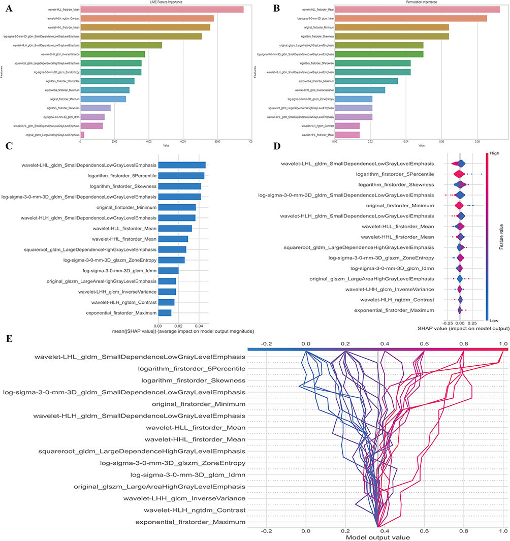Figure 7 Model interpretation using the LIME and SHAP framework. (A) Ranking feature importance using the LIME technique; (B) Ranking feature importance using permutation feature importance (PFI); (C) Ranking the relevance of features based on SHAP values obtained from the test set. A feature is deemed more significant if its average SHAP value is higher; (D) A summary plot illustrating the decision-making process of the radiomics model and the interactions among radiomics characteristics. Positive SHAP scores indicate a higher likelihood of correctly predicting PS, while a higher risk of PS is associated with a high value. Each point on the plot represents a patient’s forecast; (E) A decision graphic demonstrating the prediction of PS using the radiomics model. The plot shows the model’s base value and the SHAP values for each feature, highlighting the impact of each feature on the overall PS forecast as you move from bottom to top. The discrete dots on the right represent different eigenvalues, with the color indicating the magnitude of the eigenvalues (red for high and blue for low). The X-axis represents the SHAP value. In binary classification, the SHAP value can be seen as the size of the probability value influencing the model’s predicted outcome. It can also be interpreted as the extent to which each feature value influences the likelihood of a patient having PS. A positive SHAP value indicates an increased probability of PS, while a negative SHAP value suggests a decreased probability of PS (implying a likelihood of BS). Abbreviations: LIME, local interpretable model-agnostic explanations; SHAP, SHapley Additive exPlanations.

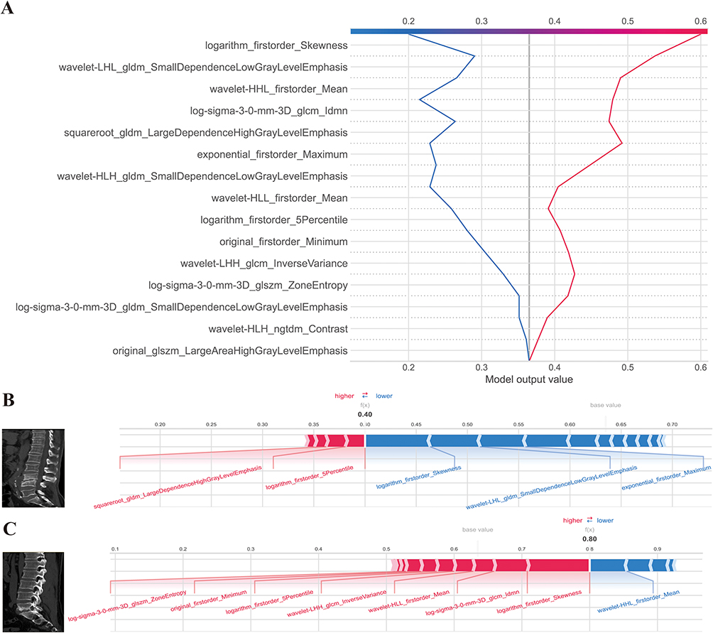Figure 8 SHAP decision and force plots. (A) Represents the SHAP decision plot for two patients in the testing set, where one is predicted with PS, and the other is predicted with BS; (B) Indicating the SHAP force plot for the PS patient, while the figure; (C) provides the SHAP force plot for the BS patient. Both patients presented with vertebral bone destruction, with one case observed at the L4-5 level and the other at the L5-S1 level. The destruction was characterized by the presence of bone hyperplasia and sclerosis along the edges. Particularly noteworthy is the predominant localization of the observed destruction along the intervertebral disc, implying a potential interplay between disc pathology and the underlying pathogenesis of the condition. The two-single case (one patient with PS and one patient with BS) prediction method was also shown in Figure 8A. Also, we offer two common instances to demonstrate the model’s interpretability: respectively, PS and BS patients. Each factor’s impact on prediction is shown with an arrow. According to the blue and red arrows, PS risk was either decreased (blue) or raised (red) by the factor. Abbreviations: LIME, local interpretable model-agnostic explanations; SHAP, SHapley Additive exPlanations.

Discussion

Accurate diagnose between PS and BS was of critical importance before treatment, because accurate diagnosis correlates with appropriate treatment option, determine treatment duration, select right antibiotics and manage complication.²¹ However, both PS and BS showed similar clinical symptoms such as fatigue, fever, back pain and weight loss. Inflammatory biomarkers, such as erythrocyte sedimentation rate, C-reactive protein and white blood cell account can be elevated in both PS and BS. In addition, both illnesses showed similar patterns of vertebral body involvement, like vertebral destruction, erosion, collapse paraspinal abscesses on CT imaging, therefore it was challenging to distinguish between them based routine CT features.^55,56 Biopsy procedures can be conducted under CT guidance to obtain samples for histological examinations and facilitate germ isolation/culture. This approach was particularly applicable for patients who do not require surgical intervention. Consequently, there was a pressing need to identify novel biomarkers that enable non-invasive diagnostic procedures, circumventing the requirement for CT-guided biopsy.

In the present investigation, we developed and evaluated an interpretable Machine Learning (ML) risk stratification tool to differentiate between PS and BS. Out of the nine ML classifiers implemented, K-Nearest Neighbors (KNN) demonstrated satisfactory performance in both the training set (AUC = 0.91) and testing set (AUC = 0.87); along with a relatively low loss value (Brier loss = 0.133, Log loss = 0.399). These promising findings underscore the potential of ML for enhancing the risk assessment procedure in clinical settings. Furthermore, using SHAP values and plots, the ML approach helped us identify crucial features. The cumulative importance of domain-specific features is illustrated and the visualization of feature significance can lend intuitive insights to physicians and enhance their understanding of the key features identified by KNN.

Radiomics analysis involved extracting a total of 15 radiomics features from medical images, which can be categorized into five groups. These categories were first-order features (6); Gray Level Co-occurrence Matrix (GLCM) features (2); Gray-Level Dependence Matrix (GLDM) features (4); Gray-Level Size Zone Matrix (GLSZM) features (2); and Neighborhood Gray Tone Difference Matrix (NGTDM) features (1). By analyzing these features, valuable insights can be gained regarding voxel intensities, texture patterns, and spatial distribution within the image. Using widely known and fundamental metrics, the first-order features primarily characterized the distribution of voxel intensities inside the picture region indicated by the mask. The grey-level relationships within an image were quantified by the GLDM features. The grey-level zones in an image were quantified by the GLSZM features. Coroller et al conducted a study to investigate whether pre-treatment radiomics data could predict the pathological response following neoadjuvant chemoradiation in patients with locally advanced non-small cell lung cancer; the results showed that first-order feature (wavelet HLL mean) was the only significantly predictive feature with an AUC of 0.63, which was found to be one of the significant features in our study.⁵⁷ Ma et al evaluated the potential value of radiomics features obtained from non-contrast computed tomography (NCCT) to detect acute aortic syndrome (AAS) images; they found nine radiomic features, which also included wavelet LLH mean feature, and SVM algorithm showed best performance 0.997 (95% CI, 0.992–1).⁵⁸ Furthermore, our findings were consistent with the study conducted by Wang et al, where they also identified several important features, including small dependence low gray-level emphasis, that can be utilized to predict the pretreatment CD8+ T-cell infiltration status in primary head and neck squamous cell carcinoma.⁵⁹ Ren et al conducted a study which showed that multimodal radiomics can distinguish between true tumor recurrence (TuR) and treatment-related effects (TrE) in glioma patients with high accuracy (AUC: 0.965 ± 0.069).⁶⁰ Our findings were consistent with this study, as we also found that wavelet HLL ngtdm contrast was a meaningful feature in identifying BS versus PS.

Machine learning models have been widely used in the medical field, from disease diagnosis and prognosis, to medical image analysis and personalized therapy. However, due to its complexity and difficult understanding how to arrive at their decision, machine learning also referred as black box model.⁶¹ Features like wavelet HLL mean, wavelet HLL ngtdm contrast, and small dependence low gray-level emphasis can be explained as having various rank statuses by these different interpretation algorithms. LIME-Local Interpretable Model-Agnostic Explanations, the LIME technique generates comprehensible justifications for each prediction made by intricate machine learning models. To help comprehend the reasons impacting the model’s conclusion, LIME outputs feature significance weights that show how much each feature contributes to the prediction for that particular instance.⁶² LIME model showed top 3 important features are wavelet HLL first-order mean, wavelet HLH ngtdm contrast and wavelet HHL first-order mean. Permutation feature importance (PFI) is a method for calculating how important various variables or features are in a machine learning model. The method involves arbitrarily varying a certain feature’s values and assessing the resulting shift in the predicted accuracy or model performance. When a feature is permuted, indicating that the feature is important and that the model significantly depends on it for correct predictions.⁵² In our study, top 3 important features indicated by PFI are wavelet HLL first-order mean, logsigma3-0-mm-3D-glcm-Idmn and original first-order minimum Value of the Shapley Additive Explanation (SHAP)-game theory is used by SHAP, a unified framework, to explain any machine learning model’s predictions. Every feature is given a value that represents its contribution to the prediction. With regard to explaining individual predictions, SHAP values offer a globally consistent method that emphasizes the significance of each characteristic in relation to other factors.⁶³ In the present research, SHAP model showed the most important features are wavelet LHL gldrm Small Dependence Low Gray-Level Emphasis, logarithm first-order 5Percentile, and logarithm first-order Skewness. The results revealed disparate rankings for features among the three interpretation models. Therefore, we recommend employing multiple-interpretation algorithms to inform decision-making processes.

Furthermore, important machine learning procedure called cross-validation divides data into training and testing sets in order to calculate the generalization accuracy of a classifier for a given dataset. To encompass feature selection and parameter tuning, it has been expanded in a variety of ways. Incorporating feature selection and machine learning parameter modification to train the best prediction model using nested CV is efficient.⁶⁴ In our study, we used nested cross validation and achieved excellent performance of the models.

Limitation

To the best of our knowledge, this study is the first to employ a radiomics combined machine learning method to distinguish between Brucella spondylitis and pyogenic spondylitis. However, there are some limitations in our study. Firstly, due to its retrospective nature and being conducted at a single center, our sample size remained relatively small despite collecting materials over a 5-year period and we did not have external validation set. Therefore, future investigations should aim for larger sample sizes and involve multiple centers, include external validation sets. Secondly, the retrospective design of the study may have been influenced by case selection bias, potentially impacting the results. Thirdly, the performance of the developed model could be influenced by the choice of feature selection algorithm. Unfortunately, we were unable to accurately optimize the final selected features as we did not incorporate dimensionality reduction algorithms or employ cross-validation procedures in multiple classifiers. This limitation might have resulted in an inadequate selection of final features. Lastly, in our research due to this is a preliminary study that focused the radiomics features potential, qualitative evaluation features have not included, further we will expand our criteria and incorporate more useful information.

Conclusion

In conclusion, the presented radiomics machine-learning classifier demonstrates excellent predicted accuracy and stability. It offers a non-invasive approach to identify Brucella spondylitis and pyogenic spondylitis before clinical intervention. The radiomics combined machine learning model can provide valuable information for clinicians.

References

1. Kourbeti IS, Tsiodras S, Boumpas DT. Spinal infections: evolving concepts. Curr Opin Rheumatol. 2008;20(4):471–479. doi:10.1097/BOR.0b013e3282ff5e66
2. Hopkinson N, Patel K. Clinical features of septic discitis in the UK: a retrospective case ascertainment study and review of management recommendations. Rheumatol Int. 2016;36(9):1319–1326. doi:10.1007/s00296-016-3532-1
3. Davis DP, Wold RM, Patel RJ, et al. The clinical presentation and impact of diagnostic delays on emergency department patients with spinal epidural abscess. J Emerg Med. 2004;26(3):285–291. doi:10.1016/j.jemermed.2003.11.013
4. Kehrer M, Pedersen C, Jensen TG, Lassen AT. Increasing incidence of pyogenic spondylodiscitis: a 14-year population-based study. J Infect. 2014;68(4):313–320. doi:10.1016/j.jinf.2013.11.011
5. Heidari B, Heidari P. Rheumatologic manifestations of brucellosis. Rheumatol Int. 2011;31(6):721–724. doi:10.1007/s00296-009-1359-8
6. Pappas G, Papadimitriou P, Akritidis N, Christou L, Tsianos EV. The new global map of human brucellosis. Lancet Infect Dis. 2006;6(2):91–99. doi:10.1016/S1473-3099(06)70382-6
7. Alp E, Doganay M. Current therapeutic strategy in spinal brucellosis. Int J Infect Dis. 2008;12(6):573–577. doi:10.1016/j.ijid.2008.03.014
8. Lee KY. Comparison of pyogenic spondylitis and tuberculous spondylitis. Asian Spine J. 2014;8(2):216–223. doi:10.4184/asj.2014.8.2.216
9. Park JH, Shin HS, Park JT, Kim TY, Eom KS. Differentiation between tuberculous spondylitis and pyogenic spondylitis on MR imaging. Korean J Spine. 2011;8(4):283–287. doi:10.14245/kjs.2011.8.4.283
10. Aljawadi A, Jahangir N, Jeelani A, et al. Management of pyogenic spinal infection, review of literature. J Orthop. 2019;16(6):508–512. doi:10.1016/j.jor.2019.08.014
11. Babic M, Simpfendorfer CS. Infections of the Spine. Infect Dis Clin North Am. 2017;31(2):279–297. doi:10.1016/j.idc.2017.01.003
12. Sanodze L, Bautista CT, Garuchava N, et al. Expansion of brucellosis detection in the country of Georgia by screening household members of cases and neighboring community members. BMC Public Health. 2015;15:459. doi:10.1186/s12889-015-1761-y
13. Berbari EF, Kanj SS, Kowalski TJ, et al. 2015 Infectious Diseases Society of America (IDSA) clinical practice guidelines for the diagnosis and treatment of native vertebral osteomyelitis in adults. Clin Infect Dis. 2015;61(6):e26–46. doi:10.1093/cid/civ482
14. Dufour V, Feydy A, Rillardon L, et al. Comparative study of postoperative and spontaneous pyogenic spondylodiscitis. Semin Arthritis Rheum. 2005;34(5):766–771. doi:10.1016/j.semarthrit.2004.08.004
15. Zhang T, Wang Y, Li Y, et al. The outer membrane proteins based seroprevalence strategy for Brucella ovis natural infection in sheep. Front Cell Infect Microbiol. 2023;13:1189368. doi:10.3389/fcimb.2023.1189368
16. Yee DK, Samartzis D, Wong YW, Luk KD, Cheung KM. Infective spondylitis in Southern Chinese: a descriptive and comparative study of ninety-one cases. Spine (Phila Pa 1976). 2010;35(6):635–641. doi:10.1097/BRS.0b013e3181cff4f6
17. Mangalgi S, Sajjan A. Comparison of three blood culture techniques in the diagnosis of human brucellosis. J Lab Physicians. 2014;6(1):14–17. doi:10.4103/0974-2727.129084
18. Kim CJ, Kang SJ, Choe PG, et al. Which tissues are best for microbiological diagnosis in patients with pyogenic vertebral osteomyelitis undergoing needle biopsy? Clin Microbiol Infect. 2015;21(10):931–935. doi:10.1016/j.cmi.2015.06.021
19. Franco MP, Mulder M, Gilman RH, Smits HL. Human brucellosis. Lancet Infect Dis. 2007;7(12):775–786. doi:10.1016/S1473-3099(07)70286-4
20. Yilmaz MH, Mete B, Kantarci F, et al. Tuberculous, brucellar and pyogenic spondylitis: comparison of magnetic resonance imaging findings and assessment of its value. South Med J. 2007;100(6):613–614. doi:10.1097/SMJ.0b013e3180600eaa
21. Li T, Liu T, Jiang Z, Cui X, Sun J. Diagnosing pyogenic, Brucella and tuberculous spondylitis using histopathology and MRI: a retrospective study. Exp Ther Med. 2016;12(4):2069–2077. doi:10.3892/etm.2016.3602
22. Lim KB, Kwak YG, Kim DY, Kim YS, Kim JA. Back pain secondary to Brucella spondylitis in the lumbar region. Ann Rehabil Med. 2012;36(2):282–286. doi:10.5535/arm.2012.36.2.282
23. Bagheri AB, Ahmadi K, Chokan NM, et al. The diagnostic value of MRI in Brucella spondylitis with comparison to clinical and laboratory findings. Acta Inform Med. 2016;24(2):107–110. doi:10.5455/aim.2016.24.107-110
24. Cowan AJ, Green DJ, Kwok M, et al. Diagnosis and management of multiple myeloma: a review. JAMA. 2022;327(5):464–477. doi:10.1001/jama.2022.0003
25. Liu X, Zheng M, Jiang Z, et al. Computed tomography imaging characteristics help to differentiate pyogenic spondylitis from brucellar spondylitis. Eur Spine J. 2020;29(7):1490–1498. doi:10.1007/s00586-019-06214-8
26. Durand DJ, Robertson CT, Agarwal G, et al. Expert witness blinding strategies to mitigate bias in radiology malpractice cases: a comprehensive review of the literature. J Am Coll Radiol. 2014;11(9):868–873. doi:10.1016/j.jacr.2014.05.001
27. Yip SS, Aerts HJ. Applications and limitations of radiomics. Phys Med Biol. 2016;61(13):R150–66. doi:10.1088/0031-9155/61/13/R150
28. Hosny A, Parmar C, Quackenbush J, Schwartz LH, Aerts H. Artificial intelligence in radiology. Nat Rev Cancer. 2018;18(8):500–510. doi:10.1038/s41568-018-0016-5
29. Lambin P, Leijenaar RTH, Deist TM, et al. Radiomics: the bridge between medical imaging and personalized medicine. Nat Rev Clin Oncol. 2017;14(12):749–762. doi:10.1038/nrclinonc.2017.141
30. Sidey-Gibbons JAM, Sidey-Gibbons CJ. Machine learning in medicine: a practical introduction. BMC Med Res Methodol. 2019;19(1):64. doi:10.1186/s12874-019-0681-4
31. Deo RC. Machine learning in medicine. Circulation. 2015;132(20):1920–1930. doi:10.1161/CIRCULATIONAHA.115.001593
32. Wang Y, Fan Y, Bhatt P, Davatzikos C. High-dimensional pattern regression using machine learning: from medical images to continuous clinical variables. Neuroimage. 2010;50(4):1519–1535. doi:10.1016/j.neuroimage.2009.12.092
33. Lao Z, Shen D, Xue Z, Karacali B, Resnick SM, Davatzikos C. Morphological classification of brains via high-dimensional shape transformations and machine learning methods. Neuroimage. 2004;21(1):46–57. doi:10.1016/j.neuroimage.2003.09.027
34. Parmar C, Grossmann P, Bussink J, Lambin P, Aerts HJWL. Machine learning methods for quantitative radiomic biomarkers. Scientific Reports. 2015;5:ARTN 13087. doi:10.1038/srep13087
35. Leger S, Zwanenburg A, Pilz K, et al. A comparative study of machine learning methods for time-to-event survival data for radiomics risk modelling. Sci Rep. 2017;7(1):13206. doi:10.1038/s41598-017-13448-3
36. Gao M, Sun J, Jiang Z, et al. Comparison of tuberculous and Brucellar spondylitis on magnetic resonance images. Spine (Phila Pa 1976). 2017;42(2):113–121. doi:10.1097/BRS.0000000000001697
37. Castella C, Kinkel K, Eckstein MP, Sottas PE, Verdun FR, Bochud FO. Semiautomatic mammographic parenchymal patterns classification using multiple statistical features. Acad Radiol. 2007;14(12):1486–1499. doi:10.1016/j.acra.2007.07.014
38. Moudgalya SS, Wilson K, Zhu X, et al. Cochlear pharmacokinetics - micro-computed tomography and learning-prediction modeling for transport parameter determination. Hear Res. 2019;380:46–59. doi:10.1016/j.heares.2019.05.009
39. Fornacon-Wood I, Mistry H, Ackermann CJ, et al. Reliability and prognostic value of radiomic features are highly dependent on choice of feature extraction platform. Eur Radiol. 2020;30(11):6241–6250. doi:10.1007/s00330-020-06957-9
40. Wang T, Bezerianos A, Cichocki A, Li J. Multikernel capsule network for schizophrenia identification. IEEE Trans Cybern. 2022;52(6):4741–4750. doi:10.1109/TCYB.2020.3035282
41. Zhang J, Wang G, Ren J, et al. Multiparametric MRI-based radiomics nomogram for preoperative prediction of lymphovascular invasion and clinical outcomes in patients with breast invasive ductal carcinoma. Eur Radiol. 2022;32(6):4079–4089. doi:10.1007/s00330-021-08504-6
42. Leger S, Zwanenburg A, Leger K, et al. Comprehensive analysis of tumour sub-volumes for radiomic risk modelling in locally advanced HNSCC. Cancers (Basel). 2020;12(10). doi:10.3390/cancers12103047
43. Tibshirani R. Regression shrinkage and selection via the lasso: a retrospective. J R Stat Soc B. 2011;73:273–282. doi:10.1111/j.1467-9868.2011.00771.x
44. Maalouf M, Trafalis TB. Robust weighted kernel logistic regression in imbalanced and rare events data. Comput Stat Data Anal. 2011;55(1):168–183. doi:10.1016/j.csda.2010.06.014
45. Chang LY, Wang HW. Analysis of traffic injury severity: an application of non-parametric classification tree techniques. Accid Anal Prev. 2006;38(5):1019–1027. doi:10.1016/j.aap.2006.04.009
46. Gislason PO, Benediktsson JA, Sveinsson JR. Random forests for land cover classification. Pattern Recogn Lett. 2006;27(4):294–300. doi:10.1016/j.patrec.2005.08.011
47. Punmiya R, Choe S. Energy theft detection using gradient boosting theft detector with feature engineering-based preprocessing. IEEE Trans Smart Grid. 2019;10(2):2326–2329. doi:10.1109/Tsg.2019.2892595
48. Noble WS. What is a support vector machine? Nat Biotechnol. 2006;24(12):1565–1567. doi:10.1038/nbt1206-1565
49. Gomez-Chova L, Camps-Valls G, Munoz-Mari J, Calpe J. Semisupervised image classification with Laplacian support vector machines. IEEE Geosci Remote Sens. 2008;5(3):336–340. doi:10.1109/Lgrs.2008.916070
50. Xie YX, Zhu CY, Zhou W, Li ZD, Liu X, Tu M. Evaluation of machine learning methods for formation lithology identification: a comparison of tuning processes and model performances. J Petrol Sci Eng. 2018;160:182–193. doi:10.1016/j.petrol.2017.10.028
51. Parvandeh S, Yeh HW, Paulus MP, McKinney BA. Consensus features nested cross-validation. Bioinformatics. 2020;36(10):3093–3098. doi:10.1093/bioinformatics/btaa046
52. Altmann A, Tolosi L, Sander O, Lengauer T. Permutation importance: a corrected feature importance measure. Bioinformatics. 2010;26(10):1340–1347. doi:10.1093/bioinformatics/btq134
53. Lundberg SM, Lee S-I A unified approach to interpreting model predictions.
54. Shapley L. Quota solutions op n-person games1. Edited by Emil Artin and Marston Morse; 1953:343.
55. Sato K, Yamada K, Yokosuka K, et al. Pyogenic spondylitis: clinical features, diagnosis and treatment. Kurume Med J. 2019;65(3):83–89. doi:10.2739/kurumemedj.MS653001
56. Bodur H, Erbay A, Colpan A, Akinci E. Brucellar spondylitis. Rheumatol Int. 2004;24(4):221–226. doi:10.1007/s00296-003-0350-z
57. Coroller TP, Agrawal V, Narayan V, et al. Radiomic phenotype features predict pathological response in non-small cell lung cancer. Radiother Oncol. 2016;119(3):480–486. doi:10.1016/j.radonc.2016.04.004
58. Ma Z, Jin L, Zhang L, et al. Diagnosis of acute aortic syndromes on non-contrast CT images with radiomics-based machine learning. Biology (Basel). 2023;12(3). doi:10.3390/biology12030337
59. Wang CY, Ginat DT. Preliminary computed tomography radiomics model for predicting pretreatment CD8+ T-cell infiltration status for primary head and neck squamous cell carcinoma. J Comput Assist Tomogr. 2021;45(4):629–636. doi:10.1097/RCT.0000000000001149
60. Ren J, Zhai X, Yin H, et al. Multimodality MRI radiomics based on machine learning for identifying true tumor recurrence and treatment-related effects in patients with postoperative glioma. Neurol Ther. 2023;12(5):1729–1743. doi:10.1007/s40120-023-00524-2
61. Petch J, Di S, Nelson W. Opening the black box: the promise and limitations of explainable machine learning in cardiology. Can J Cardiol. 2022;38(2):204–213. doi:10.1016/j.cjca.2021.09.004
62. Shin J. Feasibility of local interpretable model-agnostic explanations (LIME) algorithm as an effective and interpretable feature selection method: comparative fNIRS study. Biomed Eng Lett. 2023;13(4):689–703. doi:10.1007/s13534-023-00291-x
63. Nohara Y, Matsumoto K, Soejima H, Nakashima N. Explanation of machine learning models using shapley additive explanation and application for real data in hospital. Comput Methods Programs Biomed. 2022;214:106584. doi:10.1016/j.cmpb.2021.106584
64. Spertus JA, Fine JT, Elliott P, et al. Mavacamten for treatment of symptomatic obstructive hypertrophic cardiomyopathy (EXPLORER-HCM): health status analysis of a randomised, double-blind, placebo-controlled, Phase 3 trial. Lancet. 2021;397(10293):2467–2475. doi:10.1016/s0140-6736(21)00763-7
© 2023 The Author(s). This work is published and licensed by Dove Medical Press Limited. The
full terms of this license are available at https://www.dovepress.com/terms
and incorporate the Creative Commons Attribution
- Non Commercial (unported, 3.0) License.
By accessing the work you hereby accept the Terms. Non-commercial uses of the work are permitted
without any further permission from Dove Medical Press Limited, provided the work is properly
attributed. For permission for commercial use of this work, please see paragraphs 4.2 and 5 of our Terms.