Stochasticity among Victims of COVID-19 Pandemic

Introduction

In the literature, the term heterogeneity echoes differently in one context versus another. Its root word lies in Greek “heterogenes” meaning different. In scientific disciplines, the word heterogeneity is popularly mentioned to have existed when the variance is large. In insurance applications, for example, the premium is assessed more if an insurer is in a heterogeneous group with high hazard proneness.⁵ The large (small) variance is indicative of heterogeneity (homogeneity). Ecochard⁶ has interesting discussions for heterogeneity. In healthcare disciplines, heterogeneity is referred to as different outcomes among patients. The utilized mathematical expressions are eased in this section with added descriptions. The main topic is all about detecting reasons for complex infectivity of COVID-19 and they squarely connect to their heterogeneity. There are two types of heterogeneity. One is the observable heterogeneity, and the other is non-observable heterogeneity. We have devised a novel method to identify and estimate the level of each type in this article. The heterogeneity is linked with a non-observable hidden trait as done in genetics. The heterogeneity refers dissimilar attributes across the subgroups of the population itself even before sampling. In a sense, the heterogeneity really points to the non-identical nature in a random sample or population. Sometimes, the heterogeneity implies a shifting stochasticity. In genetic studies, several authors refer to genetic heterogeneity as rather too difficult to ascertain. They really mean that because the alleles in more than one locus exhibit susceptibility to any disease including COVID-19, there is a need to track the loci to infer their heterogeneity. So, in a sense, the application of heterogeneity is really a discussion of an opposite to similarity across loci. The reader is referred to Elston et al (2002, pages 3404–344) for details.² Hope and Norris⁷ attempted to determine how heterogeneity played a role in judgements in the context of crime victimization. A formal definition of heterogeneity is examined later in the article and its properties are explored and itemized.

We use the notations y, θ, and H₀ to describe the observation, the unknown parameter, and the posed conjecture (in other words, hypothesis) pertinent to the chance-oriented mechanism behind the COVID-19 pandemic. However, in the literature, using a random sample from a population whose main parameter is θ, when the null hypothesis is tested, it is named the homogeneity test. This suggests that heterogeneity is really all about a shifting population. This creates more confusion. The source of such confusion with respect to heterogeneity emanates from its ill-communication. It is evident that there is a lack of a clear definition of heterogeneity given by Hunink et al (Chapter 12),⁸ for details. Neither the Encyclopedia of Statistical Sciences nor the Encyclopedia of Biostatistics has even an entry as if it is not pertinent in statistical disciplines.

One comes across different types of data in scientific studies. Drawing data from a binomial population is one of them and the data should possess an under dispersion (ie, variance of the binomial distribution is smaller than its mean).¹ From a Poisson population, the drawn random sample ought to reflect equality between the mean and variance. When the main (incidence rate) parameter of a Poisson chance mechanism is stochastically transient, the unconditional observation of the random variable convolutes to an inverse binomial model.⁹ The inverse binomial distribution is known to attest that the variance is larger than its mean (Stuart and Ord¹⁰ for details). Consequently, a comparison between the mean and variance characterizes only which type of binomial, Poisson, or inverse binomial possesses the underlying chance mechanism we are sampling from but does not inform anything about heterogeneity. Recently, Hassen et al¹¹ employed a statistical concept behind a stochastic hybrid Susceptible–Infectious–Removed (SIR) framework in a Poisson chance mechanism for COVID-19 evolution and transmission in the Maghreb Central Regions (which consists of Tunisia, Algeria, and Morocco) in Western Africa. The COVID-19 pandemic is virulent and rapidly spreading in Maghreb Central Regions as much as elsewhere in other parts of the world. Their version of the SIR-Poisson model successfully predicted the range of the future infected cases since its emergence until the end of the confinement period April 2020. They estimated an average number of two contacts in Tunisia, while it was three contacts in Algeria and Morocco by an infected individual. According to them, the pandemics declined in each of the three countries but did not end. Furthermore, they detected an evolutionary change in the sense that the pandemics spreaded more rapidly in Morocco and Algeria than in Tunisia, though the most affected country was Algeria with more deaths despite a high number of cures.

With details about the probabilistic patterns among coronavirus confirmed, recovered or cured people and those that succumb as fatalities/deaths in the 32 states/territories of India are given by Shanmugam.¹³ To track the confusion with respect to heterogeneity, let us consider the data given in Table 1,¹² describing the spread of COVID-19 among the voyagers in a Diamond Princess cruise ship, during the month of February 2020. The random variables Y₁, Y₂, and Y₃ denote, respectively, the number of COVID-19 cases, the number of asymptomatic cases and the number of symptomatic cases among them in time (date). Under a given COVID-19’s prevalence rate, λ>0, the number Y₁ perhaps follows a Poisson probability pattern. For a given number of COVID-19 cases in a date, the number Y₂ perhaps follows a binomial probability pattern with parameters , where 0<p<1 denotes the chance for a COVID-19 case to exhibit no symptom. Naturally, the number Y₃ should follow a binomial probability pattern with parameters . There is an implicitness between Y₂ and Y₃ in the sense that . There are three-time oriented groups of COVID-19 incidences in Table 1. There is an observable heterogeneity among the three groups. In such scenario, it occurs due to a non-observable (parametric) heterogeneity. In data analysis, it is important to distinguish observable versus non-observable heterogeneity. A literature search does not provide an answer to this question.

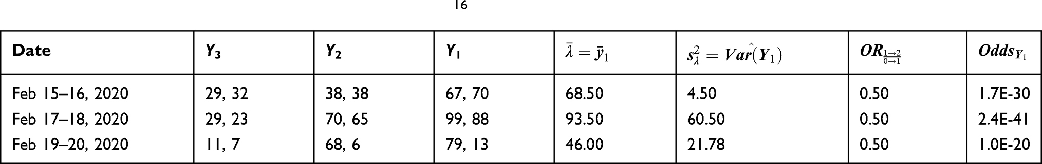Table 1 COVID-19 in Cruise Ship, 2020, Mizumoto et al16

It is evident that the average of the COVID-19 cases is an estimate of the COVID-19’s prevalence rate (ie, in Table 1). Their estimates impress that the prevalence rate is transient, not constant across every pair of two-day duration diads. The Poisson population from which the COVID-19 cases are drawn ought to have been dynamic, implying the existence of a Poisson heterogeneity. The heterogeneity can be defined and captured as follows. This is the theme and purpose in this research article.

Likewise, given that a fixed number, of COVID-19 cases has occurred, a part of them might be asymptomatic cases, and the remaining are symptomatic cases, . That is, and are complementary but . The heterogeneity in each of the two sub-binomial populations is captured in terms of the observation . We next try to define each binomial heterogeneity and compute them. In other words, we point out that the binomial heterogeneity is different from the Poisson heterogeneity. We then quantify their differences. A literature search offers no help to prove either the existence or absence of binomial heterogeneity in the data for or in Table 1. Hence, we continue probing matters with respect to heterogeneity.

The concept of heterogeneity seems to have escaped the researchers’ scrutiny for a long time. It is time well spent and worthwhile to revive an interest in the construct of heterogeneity and that is exactly what this article is trying to accomplish. Hence, we first define and construct an approach for the idea of heterogeneity. To be specific, we first discuss Poisson heterogeneity and then take up binomial heterogeneity. May be our research direction about heterogeneity is, perhaps, pioneering. However, we believe that our approach is easily extendable for many other similar methodological setups. We illustrate our definition and all derived expressions for heterogeneity using COVID-19’s data pertaining to the Diamond Princess cruise ship, Yokohama, 2020 as displayed in Table 1.

Poisson and Binomial Heterogeneities

Applied scientists emphasize that heterogeneity is of paramount importance in extracting and interpreting data evidence. Many data analysts are convinced that an unrecognized heterogeneity leads to a biased inference. To begin with, let us define heterogeneity. It is a factor causing non-similarities. In such scenario, we ought to identify its sources. We contemplate that there are two sources for heterogeneity to exist. One source ought to be from the drawn random sample of observations: , which we recognize as observable heterogeneity. The sampling variability, for a selected statistic would express the observable heterogeneity. Another source is manifested in a non-observable parameter, θ of the chance mechanism, which we recognize as non-observable heterogeneity. We wonder whether a non-uniform stochastic pattern of θ be indicative of the non-observable homogeneity. If the chance mechanism perversely selects a probability density function (pdf) for θ, how would it manifest itself to portray the non-observable heterogeneity? Both observable and non-observable heterogeneity together, ought to be involved to make any definition of heterogeneity complete. If so, how do we integrate them? Often, under/over-dispersion is confused to be heterogeneity. It seems that the over/under dispersion⁴ is precipitated by heterogeneity but not the other way. It is not obvious or proven so far in the literature on whether the converse is true. We focus only on Poisson and binomial populations to address heterogeneity and these arguments can be repeated for other populations considering similar methods.

Poisson Heterogeneity

Recall that the random integer, Y₁ denoting the number of COVID-19 cases in a place (like the Diamond Princess cruise ship) at a time (like February 2020) is a Poisson random variable with a specified prevalence rate, λ>0. That is, the conditional probability of observing number of COVID-19 cases under a prevalence rate λ>0 is with its expected number and variability . The reader is referred to Rajan and Shanmugam¹⁴ for detailed derivations of the Poisson mean and variance. The prevalence parameter λ itself is crucial in our discussions. The Poisson variability cannot be heterogeneity because the expected value also changes when the variability changes due to their inter-relatedness. Realize that no two individuals on the ship are assumed to have the same level of susceptibility to the COVID-19 virus. It is reasonable to imagine that the prevalence levels follow a conjugate, stochastic gamma distribution. The so-called conjugate prior knowledge in the Bayesian framework smooths the statistical analytic process. It is known that the conjugate prior for the Poisson distribution is gamma, whose pdf is

(1)

with an average. and variability , where the parameters α and β are recognized as hyper-parameters.¹⁴ Note that the hyperparameter α>0 causes the variability in the COVID-19’s prevalence rate to fluctuate up or down and hence, you would anticipate the heterogeneity to involve the hyperparameter α. But the question is how?

We assume that the probability of observing a non-negative COVID-19 cases, is a Poisson under a stable sampling population with an expected number and a variability . With replications, the observable heterogeneity should become estimable. That is to mention, the maximum likelihood estimate (MLE) of the COVID-19 prevalence rate is the average number, , of the observations. To discuss the non-observable heterogeneity, we need to integrate its conjugate prior for the non-observable λ with the likelihood and it results in an update and it is called posterior pdf for λ. The expressions for non-observable heterogeneity, observable heterogeneity and other expressions are derived and used.

Binomial Heterogeneity

In this section, we explore heterogeneity for two sub-binomial processes emanating from a Poisson process. The asymptomatic number, Y₂ and symptomatic number, Y₃ of COVID-19 cases are two branching binomial random numbers out of the Poisson random number, of COVID-19 cases. These two split random variables are complementary of each other in the sense that . Then, what are the underlying model for Y₂ and for Y₃? Are they correlated random variables? If so, what is their correlation? These are pursued in this section.

Let an indicator random variable, for a COVID-19 person to show asymptomatic symptom with a probability, 0<p<1 and to show symptomatic symptom with a probability, 0<1-p<1. Then, for a fixed , the random variable, follows a binomial probability distribution with parameters . Likewise, for a fixed , the random variable, follows a complementary binomial distribution with parameters . That is,

(2)

and

(3)

The expressions for non-observable heterogeneity, observable heterogeneity and other expressions are given in Appendix I.

Tango Index

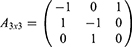
Lastly, we develop the Tango index and its significance level over the time period. Tango¹⁵ proposed an index to detect disease clusters in grouped data. This index received considerable attention in the literature. Following the line of thinking in Tango¹⁵ we could next assess the MLEs of several entities we estimated and displayed in Tables 1–3. There are three groups of duration. The group 1 consists of 15th and 16th of February 2020. The group 2 encloses data for 17th and 18th of February 2020. Group 3 contains data of 19th and 20th of February 2020. Two independent contrasts among the three groups are feasible. In an arbitrary style, we select to compare group 1 with group 2 and then group 2 with group 3. For this purpose, we formulate a contrast matrix

(4)

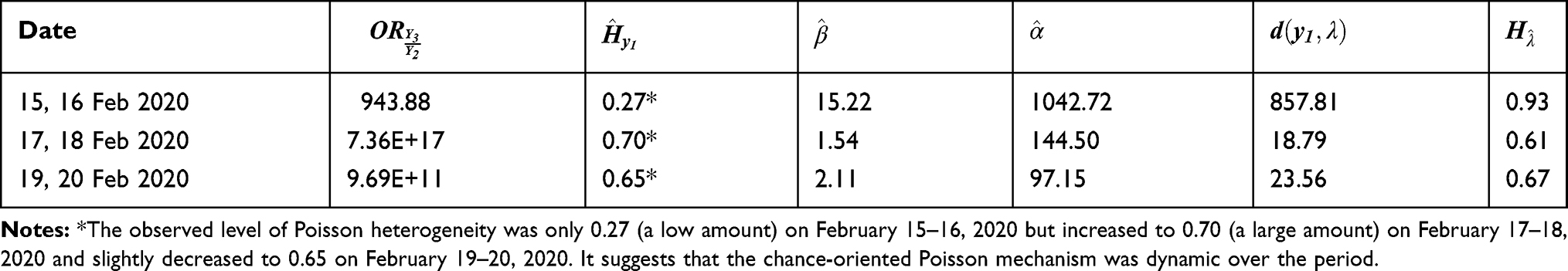Table 2 Results for Mizumoto et al’s COVID-19 Data in Diamond Princess

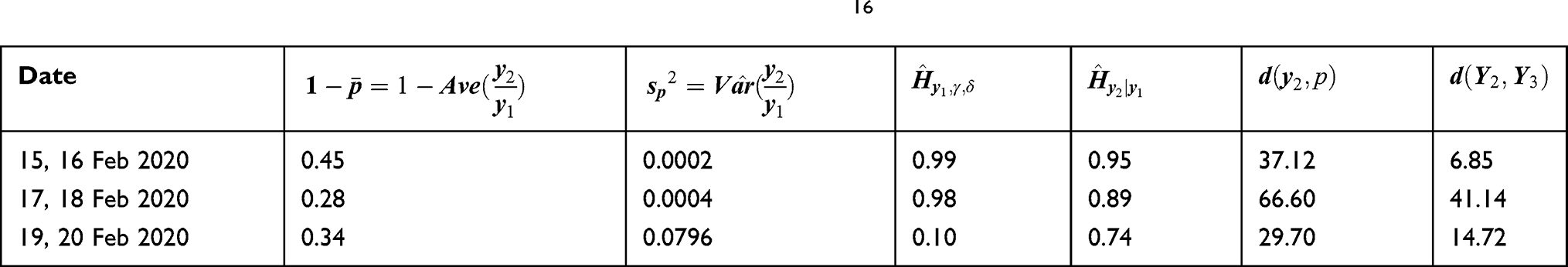Table 3 Results for Asymptomatic COVID-19 Cases in Mizumoto et al16

where the third column of the matrix needs no explanation. The Tango’s statistic T=_r′A_r follows a chi-squared distribution with v = 2 degrees of freedom (df), where _r is a row vector of the MLE of a chosen entity in our analytic results in Tables 1 or 2 or 3. For an example, let _r for the MLE of the COVID-19 prevalence rate, λ in the groups. Then, the Tango’s test statistic is T = 422.25 with v = 2 df and p-value=2.03975E-92. Likewise, the Tango’s test statistic value and its p-value are calculated and displayed in Table 4 for other entities.

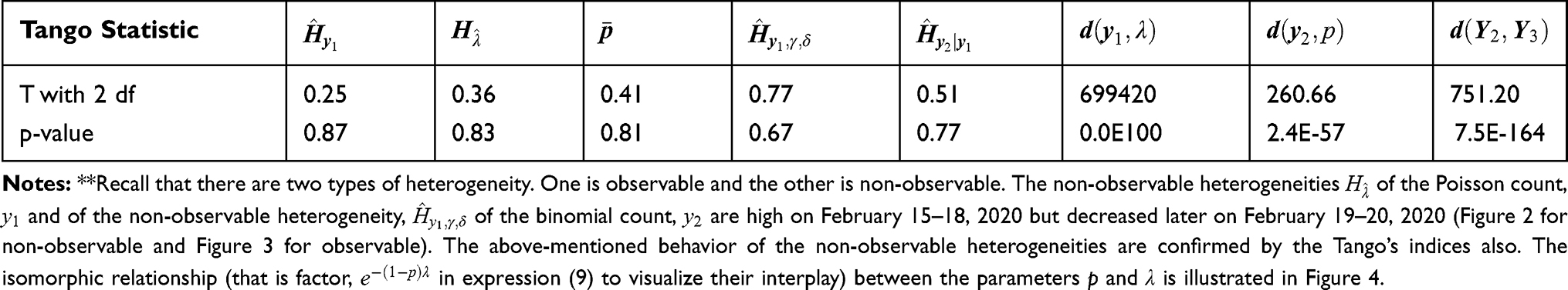Table 4 Tango’s Test Statistic** and Its P-value for Several Entities

Illustrating Using COVID-19 Data of the Diamond Princess Cruise Ship

In this section, we illustrate all the concepts and expressions of Poisson and Binomial Heterogeneities. Let us consider the COVID-19 data in Table 1 for the Diamond Princess Cruise Ship, 2020. The Diamond Princess is a cruise ship registered in Britain and operated across the globe. During a cruise that began on 20 January 2020, positive cases of COVID-19 linked to the pandemic were confirmed on the ship in February 2020. Over 700 people out of 3711 became infected (567 out of 2666 passengers and 145 out of 1045 crew), and 14 passengers died. To be specific, on the 15th of February 2020, 67 people were infected, on the 16th of February 2020, 70 people were infected, on the 17th of February 2020, there were 99 COVID-19 cases, on the 18th of February, another 88 cases were confirmed. The US government initially asked Japan to keep the passengers and crew members on board the ship for 14 days. The US government, however, changed its policy to bring them to Travis Air Force Base in California and the Base in San Antonio, Texas.

For each specified day in the first column in Table 1, the estimate of the COVID-19’s prevalence rate and its variance are calculated using expressions and . Both the prevalence and its variability increased and then decreased over the days. However, their correlation, is calculated using the observed numbers on and for each day (see in Table 2) and the estimated correlations had been stable over the days. Substituting and in the expression

(5)

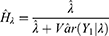
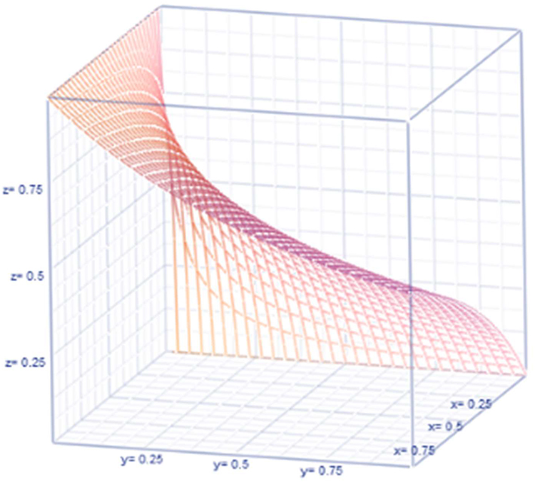
we obtained the non-observable heterogeneity and displayed in Table 2. The non-observable Poisson heterogeneity for was high in the beginning day, came down later but only to increase later. Using and in the expression

(6)

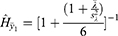
we obtained the observable heterogeneity and displayed in Table 2. The observable Poisson heterogeneity was low in the beginning day, increases and then to decrease. Note in Table 2 that the observable and non-observable Poisson heterogeneities are inversely proportional. In other words, the estimate of the shape and scale parameter in the Bayesian approach are respectively and (see their values in Table 2). The shape parameter value decreased consistently over the days. The scale parameter was high to begin with, then increased later. The distance, between the observable and non-observable Poisson mechanism for is calculated using the expression

(7)

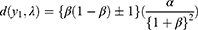
and displayed in Table 2. Notice that the distance was large to begin with, decreased then but to increase later over the days.

Note that we compute for the day. Then, we calculate the average: and the variance: , ( in Table 1) and it had been steadily increasing over the days since 15 February 2020. This is something valuable for the medical professionals learning the clinical nature of COVID-19. Using the expression,

(8)

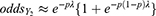
in Binomial Heterogeneity, we calculated the odds for a COVID-19 case to become an asymptomatic type and displayed in Table 2.

Likewise, using the expression

(9)

we estimated the odds for a COVID-19 case to become a symptomatic case and displayed in Table 2. Notice that both odds ( and ) are low but their odds ratio,

(10)

is not negligible but reveals that the situation is favorable to symptomatic rather than asymptomatic. This discovery is feasible because of the approach, and it is an eye-opening reality for the medical professionals in their desire to control the spread of the COVID-19 virus. Both the observable, and non-observable, binomial heterogeneity (see their values in Table 3) were decreasing for the number, of asymptomatic COVID-19 cases. The distance, between the observable and non-observable for asymptomatic cases was moderate in the beginning, then increased, and then decreased over the next days (see their values in Table 3). However, the distance, between the observable, of the asymptomatic cases and the observable, of the symptomatic cases was narrow, then wider, and then moderate over the days (their values in Table 3).

For a COVID-19 case to become a symptomatic type, the chance is moderate to less and then more over the days ( in Table 3). The estimate of the shape and scale parameter happened to be and respectively (see their values in Table 3). Both the shape parameter and the scale parameter values decreased drastically over the days. 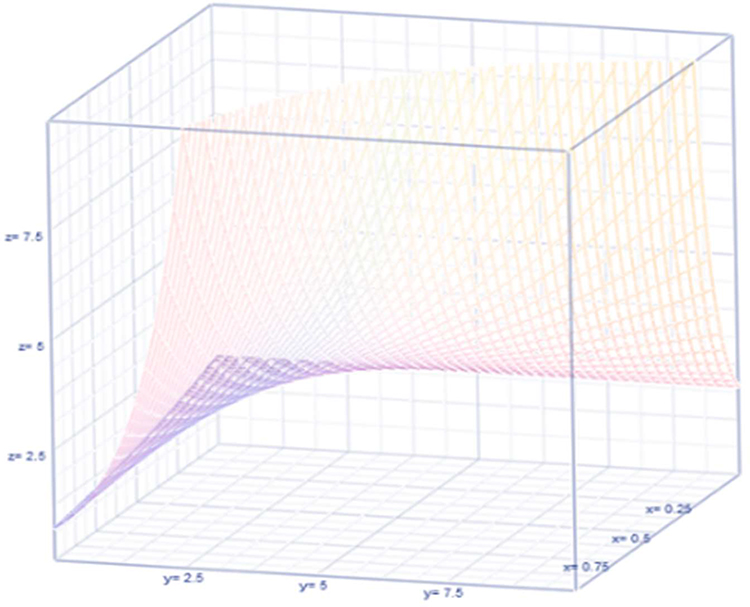From the p-values in Table 4, we infer that the prevalence rate, , the distances, , and do differ significantly over the three groups of diad days (Figure 1). The chance for COVID-19 to become an asymptomatic type does not differ significantly across the three groups. On the contrary, the non-observable heterogeneities of the Poisson random number, and of the binomial random number, are not significant. Likewise, the observable heterogeneities of the Poisson random number, and of the binomial random number, for a given are not significant.

Figure 1 Distance, in Poisson.

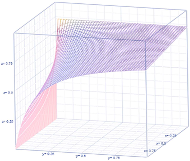Figure 2 Non-observable heterogeneity.

Figure 3 Observable heterogeneity.

Figure 4 The configuration isomorphic factor .

Discussion and Conclusion

The conclusions are reached based the new novel method that is generated in this article as there is no appropriate model or method in the literature. The sample size is sufficient. The control and experimental groups are not applicable in our discussion because of openly observed (not experimental) collection of COVID-19. The risk³ of contracting the COVID-19 virus during a cruise is more than in a community setting as confined spaces discourage non-pharmaceutical mitigation strategies such as social distancing, to be weakly implemented and, not to mention, breathing air is tightly internalized. More nations are afraid to let the voyagers come ashore at the seaports.³ Not even the ships are permitted to dock at the port as to not complicate virus mitigation efforts by the local surrounding communities. The scenario seems to be anti-humanistic. Crew members are known to have committed suicide on the ship itself. The medical doctors and/or pharmaceutical service were strained due to the infected and COVID-19 free voyagers. Lack of clear symptoms among those that were infected added to difficulties in managing the COVID-19 crisis onboard the ship, and for any ship for that matter. Most importantly, how do we dispose of the COVID-19 fatalities (bodies), in a safe manner?

Amid uncertainties about the root cause and/or the appearance of any symptoms, the best modelers can do (as it is done in this article) is to devise a methodology to address the observable as well as non-observable heterogeneity, estimate the proportion of COVID-19 cases to be asymptomatic, estimate the odds of becoming symptomatic, and the odds ratio for asymptomatic in comparison to those symptomatic among COVID-19 cases (Figure 5). Some of these are non-trivial to the professional experts dealing with the intention of reducing the spread of COVID-19 if not its total control. Still much of COVID-19 is a mysterious pandemic. It is clear that non-pharmaceutical mitigation strategies such as social distancing, utilization of face coverings, frequent hand sanitization, infected people quarantine on board, and severely controlled ship cleanliness and sanitation standards are required; this may only be successful with limited numbers of passenger and crew members. Given the nature of the disease, its heterogeneity and human social norms, pre-voyage and post-voyage quick testing procedures may become the new standard for cruise ship passengers and crew. The technological advances in testing provided today would facilitate more humanistic treatment as compared to archaic quarantine and isolation practices for all onboard ship. With quick testing, identification of those infected and thus not allowed to embark on a cruise or quarantine those disembarking, and other mitigation strategies, the popular cruise adventure could be available safely again. Whatever the procedures implemented, the methodological purpose of this study should add valuable insight in the modeling of disease and specifically, the COVID-19 virus.

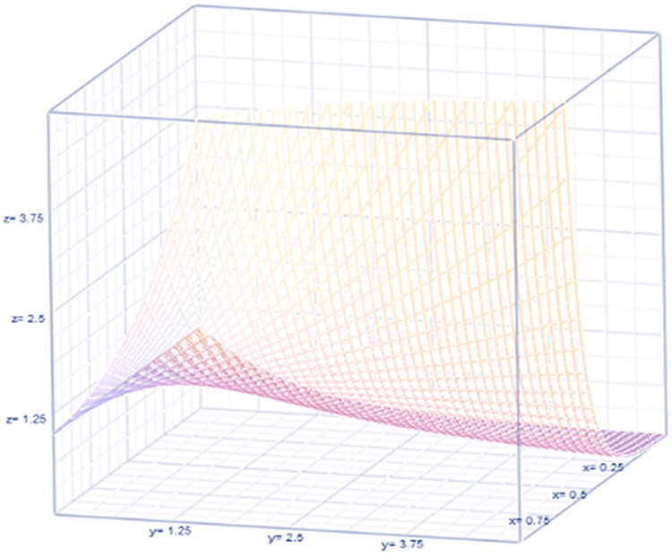Figure 5 Odds for asymptotic.

The novel method that is presented in this article offers an approach to extract the findings from any data in other disciplines also. The future research work ought to involve building data mining and/or regression fit for data with predictors on the pandemic incidences. The data collection methods could be survey or experimental design based as the method is then applicable to a variety of disciplines including marketing, sociology, business, computer information systems, communication engineering, medicine, public health, and artificial intelligence, among others.

References

1. Blumenfeld D. Operations Research Calculations Handbook. Boca Raton, Florida: CRC Press; 2020.
2. Elston R, Olson J, Palmer L. Biostatistical Genetics and Genetic Epidemiology. Baffins Lane, Chichester, West Sussex, UK: Wiley Press; 2002.
3. Khokhlov V. Conditional value-at-risk for elliptical distributions. Eur J Manag Bus Econ. 2016;2(6):70–79.
4. Shanmugam R, Radhakrishnan R. Incidence jump rate reveals over/under dispersion in count data. Int J Data Anal Inf Syst. 2011;3(1):1–8.
5. Spreeuw J. Heterogeneity in hazard rates in insurance, Tinbergen Institute of Research Series, 210 [Ph. D. thesis] Amsterdam: University of Amsterdam; 1999.
6. Ecochard J. Heterogeneity in fecundability studies: issues and modeling. Stat Methods Med Res. 2006;15:141–160. doi:10.1191/0962280206sm436oa
7. Hope T, Norris P. Heterogeneity in the frequency distribution of crime victimization. J Quant Criminol. 2013;29(4):543–576. doi:10.1007/s10940-012-9190-x
8. Hunink MG, Weinstein MC, Wittenberg E, et al. Decision Making in Health and Medicine: Integrating Evidence and Values. Cambridge, UK: Cambridge University Press; 2018.
9. Ross S. A First Course in Probability.
10. Stuart A, Ord K. Kendall’s Advanced Theory of Statistics, Volume 1. London: Oxford University Press; 2015.
11. Hassen HB, Elaoud A, Salah NB, et al. A SIR Poisson model for COVID-19 evolution and transmission inference in the Maghreb Central Regions. Arab J Sci Eng. 2021;46(1):93–102. doi:10.1007/s13369-020-04792-0
12. Mizumoto K, Chowell G. Transmission potential of the novel coronavirus (COVID-19) onboard the diamond Princess Cruises Ship, 2020. Infect Dis Model. 2020;5:264–270. doi:10.1016/j.idm.2020.02.003
13. Shanmugam R. Probabilistic patterns among coronavirus confirmed, cured and deaths in Thirty-two India’s States/Territories. Int J Ecol Econ Stat. 2020;41:45–56.
14. Rajan C, Shanmugam R. Discrete Distributions in Engineering and the Applied Sciences, Synthesis Lectures on Mathematics and Statistics. Vol. 12. 82 Winter sport Ln, Williston, VT 05495, USA: Morgan & Claypool Press; 2020:1–227.
15. Tango T. The detection of disease clustering in time. Biometrics. 1984;40:15–26. doi:10.2307/2530740
16. Mizumoto K, Kagaya K, Zarebski A, Chowell G. Estimating the asymptomatic proportion of coronavirus disease 2019 (COVID-19), cases on board the Diamond Princess cruise ship, Yokohama, 2020. Euro Surveill. 2020;25(10):1560–7917. doi:10.2807/1560-7917.ES.2020.25.10.2000180
© 2022 The Author(s). This work is published and licensed by Dove Medical Press Limited. The
full terms of this license are available at https://www.dovepress.com/terms.php
and incorporate the Creative Commons Attribution
- Non Commercial (unported, v3.0) License.
By accessing the work you hereby accept the Terms. Non-commercial uses of the work are permitted
without any further permission from Dove Medical Press Limited, provided the work is properly
attributed. For permission for commercial use of this work, please see paragraphs 4.2 and 5 of our Terms.