Random Forest Regression May Become the Optimal Regression Model for Osteoarthritis of the Knee in Elderly, in the Context of Embodied Cognition and Psychosomatic Medicine

Introduction

Regression analysis is widely used in disciplines such as medicine and psychology, and its importance is particularly prominent when dealing with longitudinal research data.^1–3 Longitudinal studies, which involve multiple measurements of variables from the same group over time, reveal the dynamic relationships between variables as they change, providing a vital statistical tool for understanding complex causal relationships. In medical research, regression analysis is employed to predict disease progression, evaluate treatment outcomes, and explore associations between risk factors and health outcomes.^3,4 In psychological research, regression analysis is often used to examine relationships between psychological states, behaviors, and environmental factors, helping researchers derive meaningful conclusions from large datasets.⁵ Despite the extensive use of regression models in both medical and psychological research, the optimal regression approach for predicting psychosomatic outcomes in patients with knee osteoarthritis (KOA) remains unclear.

Meanwhile, growing attention has been paid to embodied cognition and psychosomatic medicine in the treatment of chronic diseases. In current hospital applications, the background of embodied cognition and psychosomatic medicine is increasingly valued, especially in the treatment of chronic diseases and mental health issues.^6,7 The theory of embodied cognition highlights the central role of the body in cognitive and emotional regulation. Hospitals are starting to design more personalized and holistic treatment plans by considering not only patients’ physical responses, emotional states, and cognitive processes but also how these factors interact.^8,9 For example, in the treatment of elderly patients with chronic pain, knee osteoarthritis (KOA), or depression, doctors not only focus on medication and surgery but also incorporate physical exercises, relaxation techniques, and cognitive-behavioral therapy to help patients improve their physical condition, which in turn promotes emotional and psychological health.¹⁰ Psychosomatic medicine further emphasizes the interaction between mental and physical health, recognizing the impact of psychological factors on the onset and treatment of diseases.¹¹ This approach has led to the use of psychological interventions, meditation, and breathing exercises in hospitals to help patients manage psychological stress, improve quality of life, and enhance overall treatment outcomes. Previous studies have typically focused on the application of individual regression techniques in clinical prediction tasks. However, few studies have conducted a comparative analysis of multiple regression models specifically in the context of post-treatment psychological outcomes among elderly KOA patients. This lack of comparison represents a significant gap in the current literature.

However, such psychosomatic processes are complex and may involve nonlinear and interactive effects across multiple domains. Regression models that can effectively capture these patterns are crucial for understanding and predicting post-treatment mental health outcomes. Different types of regression methods have their own strengths and weaknesses when handling longitudinal data.^12,13 Linear regression is the simplest method and is suitable for exploring linear relationships between variables. However, when dealing with longitudinal data, it may result in biased outcomes due to its neglect of time dependence.^14–16

In contrast, non-parametric methods such as random forest regression and gradient boosting decision tree (GBDT) can capture more complex nonlinear relationships.^17–19 Although these methods excel in predictive accuracy, they may fail to fully account for the dynamic characteristics of time series in longitudinal studies due to their lack of time dependency mechanisms.^20,21 Similarly, AdaBoost regression improves prediction performance by combining multiple weak learners, but its neglect of time dependence also limits its application in longitudinal research.^22,23 Thus, selecting an appropriate regression method to analyze longitudinal data, especially in the presence of complex time effects, is a key challenge for researchers.^24,25 Despite extensive applications of regression analysis in medical and psychological research, the optimal regression model for predicting psychosomatic outcomes in KOA patients remains unclear.

Previous studies have shown that KOA patients not only suffer from physical pain but also frequently experience depression, anxiety, and sleep disorders.^10,26–28 Factors such as gender, age, anxiety, depression, pain, and sleep quality all influence the post-treatment depression of elderly knee osteoarthritis (KOA) patients.^26–30 Based on the impact of these factors on patients’ post-treatment depression, this study aims to compare several common regression methods to evaluate their strengths and weaknesses in such research, assess their predictive performance, and further validate previous conclusions.

Therefore, this study aims to systematically compare the predictive performance of five commonly used regression models—non-negative linear regression, stochastic gradient descent, AdaBoost, random forest, and GBDT—in forecasting post-treatment depression among elderly KOA patients. By examining their accuracy, error rates, and coefficient patterns, we aim to identify the most suitable model for capturing psychosomatic dynamics in longitudinal clinical data and to provide guidance for future psychosomatic research involving predictive modeling.

Research Design and Methods

Instruments

This study employed multiple scales to assess the psychological and physiological states of elderly knee osteoarthritis (KOA) patients.

First, pain intensity was measured using the Visual Analog Scale (VAS), a widely used clinical tool for pain assessment. Patients indicated their pain levels on a horizontal line, with scores ranging from 0 (no pain) to 10 (severe pain). The VAS has demonstrated good reliability and validity, making it a quick and accurate measure of subjective pain experience.^31–33

Anxiety was assessed using the Beck Anxiety Inventory (BAI), developed by Beck et al to measure the severity of various anxiety symptoms. The BAI exhibits high internal consistency, with Cronbach’s alpha ranging from 0.92 to 0.94, and possesses good convergent and discriminant validity, making it suitable for evaluating anxiety in elderly patients.^34,35

Depressive symptoms were measured using the Geriatric Depression Scale (GDS), specifically designed for the elderly and sensitive to the core symptoms of depression in older adults. The GDS has high internal consistency and test–retest reliability, with Cronbach’s alpha between 0.88 and 0.94, demonstrating its effectiveness in screening for depression among the elderly.^36,37

Sleep quality was evaluated using the Pittsburgh Sleep Quality Index (PSQI), which includes 19 items divided into 7 components to provide a comprehensive assessment of the patient’s sleep status over the past month. The PSQI has good internal consistency (Cronbach’s alpha = 0.83) and test–retest reliability (0.85) and is widely used in studies on sleep disorders and psychological health.^38,39

Sample and Data Collection

The study sample consisted of knee osteoarthritis (KOA) patients hospitalized in the Department of Orthopedics and Traumatology at the Affiliated Hospital of Southwest Medical University in Luzhou, China, between September 2023 and February 2024. Inclusion criteria were patients aged over 55 years, with clear consciousness, and able to complete the questionnaire independently. Exclusion criteria included patients with severe internal diseases, major trauma, or hospital stays of less than 7 days or more than 30 days.

A total of 234 patients were initially screened for eligibility. Of these, 144 patients met the inclusion criteria and completed the pre-treatment survey, resulting in a response rate of approximately 61.5%. During the follow-up period, 106 patients completed the post-treatment survey, indicating a follow-up rate of 73.6%. The primary reasons for non-participation in the follow-up included refusal to continue (10 patients) and loss to follow-up due to discharge or transfer (28 patients). Missing data were handled using multiple imputation methods to ensure the robustness of the analysis. All participants provided informed consent before participation. Missing data were handled using Multiple Imputation by Chained Equations (MICE), implemented in SPSS 26.0. Five imputed datasets were generated and pooled to ensure stable estimation. The imputation model included all variables used in the analysis to maintain consistency and reduce bias.

Data Processing and Regression Model Selection

Data Cleaning and Standardization

Before data analysis, the raw data were cleaned and standardized using SPSS 26.0. First, missing data and outliers were removed to ensure data integrity and accuracy. Then, all variables were standardized to eliminate differences in measurement scales, making the regression analysis more comparable. All continuous variables were standardized using z-score normalization, where each variable was transformed to have a mean of 0 and a standard deviation of 1. This was done to ensure that all predictors were on a comparable scale, minimizing bias in model training caused by differing units of measurement.

Correlation and Collinearity Analysis

Before performing regression analysis, correlation analysis was conducted using SPSS 26.0 to examine the linear relationships between variables. Pearson correlation coefficients and variance inflation factors (VIFs) were calculated to assess potential collinearity issues and provide a foundation for subsequent regression analysis. In addition to calculating the Variance Inflation Factor (VIF) for each predictor, we also examined tolerance values and pairwise Pearson correlations. While no VIF exceeded the threshold of 10, variables with VIFs above 2.5 were further reviewed. No variable was removed due to collinearity, but we retained this analysis to ensure the robustness of coefficient estimation across models.

Regression Model Selection and Evaluation

This study analyzed the influence of gender, age, pre-treatment pain, depression, anxiety, and sleep on post-treatment depression in elderly KOA patients using various regression models. Specifically, several regression methods were applied. Non-negative linear regression was implemented using the LinearRegression module in Python 3.7 (sklearn version 0.24), with the positive parameter set to True. Linear regression (SGD) and AdaBoost regression were implemented using the MLPRegressor module. Random forest regression was implemented using the RandomForestRegressor module, and GBDT regression used the GradientBoostingRegressor module. All models were implemented in Python 3.7 with sklearn version 0.24, and regression coefficients were tested using the Kruskal–Wallis test in R, with key coefficients further analyzed using Bootstrap methods.

Non-negative Linear Regression is a variant of linear regression that constrains the regression coefficients to non-negative values. This method is useful when the relationship between predictor and outcome variables is expected to be unidirectional (ie, increasing the predictor should increase the outcome). In psychological and medical research, non-negative linear regression prevents the occurrence of negative coefficients, which is crucial when interpreting certain practical issues.⁴⁰

Linear Regression: As a fundamental regression method, linear regression is suitable for exploring linear relationships between variables. However, in longitudinal data, the time dependence of the data may cause the model to miss the dynamic changes in the time series. Therefore, residual analysis was conducted to ensure the model’s reasonable interpretation of the data.^41–43

Random Forest Regression: This method enhances predictive ability by constructing multiple decision trees. Random forest performs well with high-dimensional and nonlinear data, but it lacks a mechanism for handling time dependence. To address this, lagged variables were introduced to better capture the characteristics of time series.⁴⁴

AdaBoost Regression: AdaBoost is an ensemble learning method that improves prediction accuracy by weighting multiple weak learners. Although it performs well with complex data, it also lacks time-dependence handling. Therefore, lagged variables were similarly introduced to enhance its performance in longitudinal studies.²³

Gradient Boosting Decision Tree (GBDT): GBDT offers high flexibility in handling nonlinear relationships, making it particularly suitable for datasets with complex interactions. However, as GBDT does not naturally handle time series, appropriate feature engineering was required to capture the time dynamics.⁴⁵

Model Evaluation Criteria

Coefficient of Determination (R²): Measures the explanatory power of the model on data variation. The closer the R² value is to 1, the stronger the model’s explanatory power. However, R² is not sensitive to model complexity, so other metrics should be considered when comparing models.⁴⁶

Mean Squared Error (MSE): Measures the average squared error between predicted and actual values. MSE is sensitive to large errors, highlighting significant deviations, but may amplify errors due to outliers.⁴⁷

Mean Absolute Error (MAE): Calculates the average of the absolute errors between predicted and actual values. MAE provides an intuitive understanding of errors and is less sensitive to outliers than MSE, making it suitable for situations where all errors are treated equally.⁴⁸

Results

Descriptive Statistics

In Table 1 and Figure 1, the variables involved in the study include gender (sex), age (age), pre-treatment pain (P1), pre-treatment depression (D1), pre-treatment anxiety (A1), pre-treatment sleep (S1), post-treatment pain (P2), post-treatment depression (D2), post-treatment anxiety (A2), and post-treatment sleep (S2).

Table 1 Descriptive Statistics

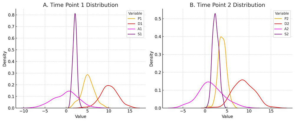Figure 1 Comparison of distributions at two time points. Notes: (A) is the time point 1 distribution; (B) is the time point 2 distribution; P1 is pre-treatment pain; D1 is pre-treatment depression; A1 is pre-treatment anxiety; S1 is pre-treatment sleep; P2 is post-treatment pain; D2 is post-treatment depression; A2 post-treatment anxiety; S2 is post-treatment sleep.

The mean value for gender (sex) is 0.2642, indicating a higher proportion of females in the sample (Table 1). The skewness is 1.085, and the kurtosis is −0.838. The mean age of participants is 59.6415 years, with a median of 60 (Table 1), suggesting a relatively concentrated age distribution (Figure 1). The skewness is −0.853, and the kurtosis is 0.849 (Table 1), indicating a relatively symmetrical age distribution with a slight negative skew (Figure 1), meaning that the sample contains a slightly higher proportion of middle-aged and elderly patients (Figure 1).

The mean pre-treatment pain score (P1) is 5.2075, with a median of 5 (Table 1), indicating that most patients experienced moderate levels of pain. The skewness is −0.564, and the kurtosis is 1.376, showing a fairly symmetrical distribution with a slight negative skew (Table 1). The mean pre-treatment depression score (D1) is 15.3208, with a median of 15 (Table 1), suggesting that patients had relatively high levels of depression. The skewness is −0.008, and the kurtosis is 0.424, indicating a symmetrical distribution (Table 1). The mean pre-treatment anxiety score (A1) is 7.7358 (Table 1), with a median of 6, indicating relatively high anxiety levels. The skewness is 4.667, and the kurtosis is 27.019, showing a highly positively skewed distribution with a significant number of extreme high scores. The mean pre-treatment sleep score (S1) is 1.8679, with a median of 2, suggesting poor sleep quality among patients. The skewness is −0.205, and the kurtosis is 0.505, indicating a symmetrical distribution (Table 1).

The mean post-treatment pain score (P2) is 2.6415, with a median of 2 (Table 1), indicating a significant reduction in pain after treatment. The skewness is 1.010, and the kurtosis is 0.568, showing a positively skewed distribution (as Table 1 and Figure 1). The mean post-treatment depression score (D2) is 10.1321, with a median of 11, indicating a decrease in depression levels (as Table 1 and Figure 1). The skewness is −0.234, and the kurtosis is −0.396, suggesting a symmetrical distribution (as Table 1 and Figure 1). The mean post-treatment anxiety score (A2) is 2.8113, with a median of 2, showing a significant reduction in anxiety levels (as Table 1 and Figure 1). The skewness is 1.611, and the kurtosis is 2.311, indicating a highly positively skewed distribution (as Table 1 and Figure 1). The mean post-treatment sleep score (S2) is 1.2667, with a median of 1, indicating improved sleep quality. The skewness is −0.065, and the kurtosis is −0.532, showing a symmetrical distribution (as Table 1 and Figure 1).

Overall, the distribution shapes of most variables meet the necessary criteria, particularly for pre-treatment depression, pre-treatment anxiety, and pre-treatment sleep, which show relatively symmetrical distributions. Therefore, standardization of the data should be performed before further analysis. The treatment appears to be effective, and the overall distribution of the data is reasonable, allowing for subsequent statistical analysis.

Correlation Analysis

Gender showed a significant positive correlation with post-treatment pain (P2) (r = 0.213, p = 0.029) (as Table 2 and Figure 2), indicating that female patients had higher post-treatment pain scores. Gender was negatively correlated with age (r = −0.270, p = 0.005), suggesting that female patients were generally younger (as Table 2 and Figure 2). Age was significantly positively correlated with pre-treatment pain (P1) (r = 0.699, p < 0.001), pre-treatment depression (D1) (r = 0.507, p < 0.001), and pre-treatment anxiety (A1) (r = 0.428, p < 0.001), indicating that older patients scored higher on these pre-treatment variables. Age was negatively correlated with post-treatment sleep (S2) (r = −0.233, p = 0.017), suggesting that older patients had lower post-treatment sleep quality scores (as Table 2 and Figure 2).

Table 2 Correlation Statistics

Figure 2 Correlation heatmap. **Correlation is significant at the 0.01 level (two-tailed). *Correlation is significant at the 0.05 level (two-tailed). P1 is pre-treatment pain; D1 is pre-treatment depression; A1 is pre-treatment anxiety; S1 is pre-treatment sleep; P2 is post-treatment pain; D2 is post-treatment depression; A2 post-treatment anxiety; S2 is post-treatment sleep.

Pre-treatment pain was significantly positively correlated with pre-treatment depression (D1) (r = 0.496, p < 0.001), pre-treatment anxiety (A1) (r = 0.582, p < 0.001), and pre-treatment sleep (S1) (r = 0.302, p = 0.002), indicating a close relationship between pain and depression, anxiety, and sleep quality (as Table 2 and Figure 2). Pre-treatment depression was significantly positively correlated with pre-treatment anxiety (A1) (r = 0.403, p < 0.001), pre-treatment sleep (S1) (r = 0.352, p < 0.001), and post-treatment pain (P2) (r = 0.201, p = 0.039), indicating a strong association between depression and anxiety, sleep quality, and pain (as Table 2 and Figure 2). Pre-treatment anxiety was significantly positively correlated with pre-treatment sleep (S1) (r = 0.311, p = 0.001) and post-treatment anxiety (A2) (r = 0.612, p < 0.001), indicating a close relationship between anxiety and sleep quality and subsequent anxiety levels (as Table 2 and Figure 2).

Pre-treatment sleep was significantly positively correlated with post-treatment sleep (S2) (r = 0.373, p < 0.001), suggesting strong consistency between pre-treatment and post-treatment sleep quality (as Table 2 and Figure 2). Post-treatment pain was significantly positively correlated with post-treatment depression (D2) (r = 0.351, p < 0.001) and post-treatment anxiety (A2) (r = 0.493, p < 0.001), indicating a close relationship between post-treatment pain and depression and anxiety (as Table 2 and Figure 2). Post-treatment depression was significantly positively correlated with post-treatment anxiety (A2) (r = 0.395, p < 0.001) and post-treatment sleep (S2) (r = 0.458, p < 0.001), indicating a close association between depression, anxiety, and sleep quality (as Table 2 and Figure 2). Post-treatment anxiety was significantly positively correlated with post-treatment sleep (S2) (r = 0.375, p < 0.001), suggesting a close relationship between anxiety and sleep quality (as Table 2 and Figure 2).

The correlation analysis results showed significant correlations between most variables, particularly those related to pain, depression, anxiety, and sleep quality. However, the high correlations between some variables (eg, age and pre-treatment pain, r = 0.699, and pre-treatment anxiety and pre-treatment depression, r = 0.582) suggest potential collinearity issues (as Table 2 and Figure 2). This collinearity may affect the independent contribution of variables in the regression analysis, leading to unstable model coefficients (as Table 2 and Figure 2). To mitigate this issue, the variance inflation factor (VIF) will be used in subsequent regression analyses to quantify the degree of collinearity, and the model will be adjusted if necessary to reduce the impact of collinearity on the results (as Table 2 and Figure 2).

Collinearity Analysis

The variance inflation factor (VIF) values from the table show that all variables have VIFs below 10 (Table 3). It is generally accepted that when the VIF is less than 10, the impact of collinearity on the regression results is considered acceptable.. In this study, most variables had VIF values well below 10, with the highest VIF being 3.861 for A2, which is still within a reasonable range (Table 3). Therefore, although some variables exhibit a degree of correlation, these correlations do not significantly negatively affect the regression analysis.

Table 3 Collinearity Analysis

Further analysis reveals that variables such as A2 (VIF = 3.861) and age (VIF = 2.693), while having slightly higher VIF values, remain within an acceptable range, indicating that their collinearity does not significantly impact the model’s stability (Table 3). The standard errors and t-values of the model also show no significant bias, suggesting that the model coefficients are robust.

In conclusion, while there is some collinearity among certain variables in this study, the overall collinearity issue is not severe and does not significantly affect the explanatory power or predictive accuracy of the regression model. The model fit remains reliable, and the conclusions are statistically meaningful.

Regression Analysis

Regression Coefficients

This study employed various regression models to analyze the data, aiming to compare the performance of different regression models in predicting the post-treatment depression (D2) of elderly knee osteoarthritis (KOA) patients and to explore the influence of each variable on depression (D2).

In the non-negative linear regression model, the coefficients for gender (sex), pre-treatment pain (P1), pre-treatment anxiety (A1), and pre-treatment sleep (S1) were 0 (Table 4). This is likely because the non-negative linear regression model enforces all regression coefficients to be non-negative. When certain variables have a negative or non-significant correlation with the dependent variable, the model is unable to express this relationship through negative coefficients, resulting in the coefficients for those variables being set to 0. Age and post-treatment sleep (S2) had a larger impact on depression (D2), with post-treatment sleep (S2) having a particularly large coefficient of 1.904 (Table 4).

Table 4 Regression

In the linear regression (SGD) model, pre-treatment depression (D1), pre-treatment anxiety (A1), and post-treatment anxiety (A2) had significant effects on depression (D2), with post-treatment sleep (S2) having the largest effect (0.741). Gender (sex) and age (age) also influenced depression, but to a lesser extent (Table 4).

In the AdaBoost regression model, post-treatment anxiety (A2) and post-treatment sleep (S2) had the greatest influence on depression (D2), indicating that these variables play a crucial role in predicting depressive states. In comparison, gender (sex) and pre-treatment anxiety (A1) had smaller effects (Table 4).

In the random forest regression model, post-treatment anxiety (A2) had the most significant impact on depression (D2), followed by pre-treatment depression (D1) and post-treatment sleep (S2) (Table 4).

In the GBDT regression model, gender (sex) and post-treatment anxiety (A2) had the largest effects on depression (D2), while the impact of other variables was relatively small (Table 4).

Kruskal–Wallis Rank-Sum Test for Regression Coefficients

The Kruskal–Wallis rank-sum test conducted on the regression coefficients showed that the test statistic (chi-squared) for all variables was 8, with p values of 0.4335. This indicates that there were no significant differences in the regression coefficients across the various regression models (Table 4).

Feature Importance Analysis

Since the Kruskal–Wallis test results were not significant, we further compared three key performance metrics: R², MSE, and MAE. Bootstrap analysis was conducted on these metrics to assess the stability and reliability of the models’ performance (Table 4).

Based on the results, although the differences in regression coefficients were not significant, the models exhibited differences in overall explanatory power (R²), prediction error (MSE), and mean absolute error (MAE). The random forest regression model performed the best, with a 95% confidence interval for R² ranging from 0.589 to 0.785, demonstrating strong explanatory power. It also had the lowest errors in MSE (confidence interval: 7.196 to 7.392) and MAE (confidence interval: 1.793 to 1.989), indicating the most accurate and robust predictive performance (as Table 5 and Figure 3).

Table 5 Comparison of Regression Model Performance

Figure 3 Comparison of R-squared, MSE, and MAE values for five regression models. Notes: 1=Non-negative Linear Regression 2=Linear Regression (SGD) 3=AdaBoost Regression 4=Random Forest Regression 5=GBDT Regression. (A) is R-squared value comparison; (B) is MSE value comparison; (C) is MAE value comparison.

In comparison, the AdaBoost regression model ranked second, with an R² confidence interval of 0.403 to 0.599. Although its performance was inferior to the random forest model, it still outperformed the other models in terms of explanatory power and predictive accuracy (as Table 5 and Figure 3). The confidence intervals for MSE and MAE were 11.506 to 11.702 and 2.519 to 2.715, respectively, showing relatively low prediction errors (as Table 5 and Figure 3).

Linear regression (SGD) and non-negative linear regression models were quite similar in terms of explanatory power and predictive accuracy. The R² confidence interval for linear regression (SGD) was 0.188 to 0.384, with an MSE confidence interval of 16.511 to 16.707 and an MAE confidence interval of 3.208 to 3.404, indicating moderate explanatory power but higher error (as Table 5 and Figure 3). The non-negative linear regression model had an R² confidence interval of 0.151 to 0.347, an MSE confidence interval of 17.375 to 17.571, and an MAE confidence interval of 3.203 to 3.399, slightly underperforming linear regression (SGD) (as Table 5 and Figure 3).

The gradient boosting decision tree (GBDT) model performed the worst, with an R² confidence interval of −0.179 to 0.017, indicating almost no explanatory power (as Table 5 and Figure 3). Its MSE confidence interval was 25.067 to 25.263, and its MAE confidence interval was 2.243 to 2.439, both significantly higher than the other models, suggesting poor predictive performance on this dataset (as Table 5 and Figure 3).

By comparing the confidence intervals and coefficient sizes, we can examine the significance of the differences between the models. Based on the R² confidence interval comparison, we can see that the intervals for non-negative linear regression (0.151, 0.347) and linear regression (0.188, 0.384) overlap (Figure 4), indicating no significant difference between the models. There is partial overlap between the intervals for linear regression and AdaBoost regression (0.403, 0.599) (Figure 4), suggesting that the models may differ significantly. The intervals for AdaBoost regression and random forest regression (0.589, 0.785) almost do not overlap (Figure 4), indicating a significant difference between the models. GBDT regression, with a negative R², may not be suitable for this dataset, and the confidence intervals show significant differences across the models.

Figure 4 Comparison of R-squared, MSE, and MAE confidence intervals for five regression models. Notes: 1=Non-negative Linear Regression 2=Linear Regression (SGD) 3=AdaBoost Regression 4=Random Forest Regression 5=GBDT Regression. (A) is R-squared confidence interval comparison; (B) is MSE confidence interval comparison; (C) is MAE confidence interval comparison.

Based on the MSE confidence interval overlap, non-negative linear regression (17.375, 17.571) and linear regression (16.511, 16.707) show little overlap (Figure 4), indicating significant differences between the models. The confidence intervals for linear regression and AdaBoost regression (11.506, 11.702) do not overlap (Figure 4), indicating a significant difference between the models. The intervals for AdaBoost regression and random forest regression (7.196, 7.392) also do not overlap, and there is no overlap between random forest regression and GBDT regression (25.067, 25.263), indicating significant differences (Figure 4).

Based on the MAE confidence interval overlap, non-negative linear regression (3.203, 3.399) and linear regression (3.208, 3.404) show complete overlap (Figure 4), indicating no significant difference between the models. There is a slight overlap between linear regression and AdaBoost regression (2.519, 2.715) (Figure 4), indicating a significant difference. There is no overlap between the confidence intervals for AdaBoost regression and random forest regression (1.793, 1.989) nor between random forest regression and GBDT regression (2.243, 2.439), indicating significant differences (Figure 4).

In summary, except for non-negative linear regression and linear regression, which showed no significant differences in overall explanatory power (R²) and mean absolute error (MAE), other models showed significant differences in R², MSE, and MAE. The random forest regression performed the best across all indicators, followed by AdaBoost regression, while GBDT regression performed the worst. These results suggest that random forest regression may be a better choice for handling similar complex psychological data.

Discussion

Multiple regression analysis is widely used in various studies, but it remains unclear which specific regression method can more accurately predict the effects of independent variables on the dependent variable in complex longitudinal psychosomatic data.² This study applied several regression models (non-negative linear regression, linear regression (SGD), AdaBoost regression, random forest regression, GBDT regression) to analyze the depression state (D2) of elderly knee osteoarthritis (KOA) patients. Based on variables such as gender, age, pain (P1 and P2), depression (D1), anxiety (A1 and A2), and sleep (S1 and S2), we explored the predictive effects of different regression models on post-treatment depression (D2). By comparing the fit statistics and Bootstrap analysis results across models, we found that while there were no significant differences in the regression coefficients, the random forest regression model performed best in terms of overall explanatory power (R²), prediction error (MSE), and mean absolute error (MAE) in predicting the depression state of KOA patients, followed by the AdaBoost regression model, while the GBDT regression model performed the worst (Figure 4).

The random forest regression model performed best in predicting the post-treatment depression state of elderly knee osteoarthritis (KOA) patients, primarily due to its ability to effectively handle complex nonlinear relationships and interactions between multiple variables. Compared to linear regression or GBDT regression models, random forest regression is more robust, able to handle outliers and missing data, and reduces the risk of overfitting, thereby improving the model’s stability and accuracy. Additionally, the ensemble learning mechanism of random forest contributes to superior performance in terms of explanatory power (R²), prediction error (MSE), and mean absolute error (MAE), making it the most accurate model in this study (as Table 5 and Figure 3).

There were two primary reasons for selecting KOA patients as the study population. First, KOA is a common disease, particularly prevalent among the elderly, making sample recruitment easier.⁴⁹ Second, previous research has shown that KOA patients often experience comorbidities such as pain, depression, anxiety, and sleep disorders, which significantly affect their quality of life and mental health.^26–30 This makes KOA patients an ideal group for studying the relationship between chronic pain and psychological issues.

The findings of this study are consistent with prior research in some aspects but also show some differences. First, many studies have identified anxiety, depression, and sleep quality as key predictors of mental health in elderly KOA patients.^26–30,49 In this study, post-treatment anxiety (A2) and post-treatment sleep (S2) had significant effects on depression (D2) across multiple models, supporting this conclusion.

However, unlike some studies, this research found that gender, age, and pre-treatment pain (P1) were not significantly associated with post-treatment depression (D2). This discrepancy may be related to the characteristics of the sample or the data processing methods used in this study. Most of the patients in this study were middle-aged and elderly women, whose pain perception and coping mechanisms may differ from those of men or younger patients. Additionally, the regression models employed in this study may be better suited to capture the complex interactions between psychological variables rather than the direct effects of individual physiological factors on psychological states. The absence of significant predictive effects for gender, age, and pre-treatment pain may reflect sample homogeneity and the stronger influence of post-treatment psychosomatic factors. These findings do not imply a lack of sensitivity in the models but rather highlight the complex interplay between demographic, clinical, and psychological variables.

The results of this study have important clinical and theoretical implications. First, the study highlights the need to focus on anxiety levels and sleep quality in psychological interventions for elderly KOA patients, as these factors have significant effects on depression. This underscores the importance of targeted interventions, such as a combination of psychotherapy and pharmacotherapy, which may be effective in alleviating depressive symptoms. Additionally, the superior performance of random forest regression suggests that complex nonlinear models can better capture underlying patterns in patient data. Therefore, appropriate statistical models should be used when analyzing complex psychological data. Future research could validate these findings by expanding the sample size and incorporating more variables, as well as exploring the applicability of different models to other medical datasets. This could provide new insights for personalized treatment plans and related research data analysis.

In terms of methodological transparency, this study employed multiple imputation using the MICE (Multiple Imputation by Chained Equations) technique to address missing data, ensuring that all variables used in the predictive models were consistently represented across imputations. This approach reduces potential bias and improves the reliability of the results. Additionally, multicollinearity was assessed using both VIF and tolerance values. Although no variables exceeded the commonly accepted VIF threshold of 10, further scrutiny was applied to those with values above 2.5 to ensure coefficient stability across models. No variable was excluded, as the collinearity was within acceptable limits. These methodological choices strengthen the robustness and replicability of the findings. Taken together, these methodological refinements, combined with the comparative modeling approach, enhance the study’s value for future research in psychosomatic medicine and for developing personalized care strategies in elderly patients with complex physical and emotional health needs.

Interestingly, some variables such as gender, age, and pre-treatment pain did not emerge as significant predictors of post-treatment depression in most models. One possible explanation is that the psychological state after treatment may be more directly influenced by post-treatment experiences (such as anxiety and sleep quality) than by baseline physiological status. Additionally, the limited variation in gender (with a predominantly female sample) and age range (mostly elderly patients) may have reduced the statistical power to detect their effects. It is also possible that the coping strategies and treatment responses among female elderly patients are more homogeneous, potentially obscuring the influence of these demographic factors.

Despite the meaningful conclusions drawn from this study, there are some limitations. First, the sample size was relatively small, focused on a specific region, and predominantly female, which may have led to some collinearity issues and limited the generalizability of the results. Future studies should expand the sample size and include patients from diverse regions and cultural backgrounds to improve the external validity of the findings. Second, although multiple regression models were applied in this study, the specific performance of each model under different data characteristics was not thoroughly explored. Future research could incorporate model interpretability analysis to better understand the differences in model performance. Moreover, this study primarily relied on questionnaire data; future studies could consider including more objective physiological indicators, such as blood pressure and glucose levels, to provide a more comprehensive assessment of patients’ health status.

Conclusion

This study compared the performance of multiple regression models—including non-negative linear regression, stochastic gradient descent, AdaBoost, gradient boosting decision trees (GBDT), and random forest regression—in predicting post-treatment depression in elderly patients with knee osteoarthritis (KOA), using psychosomatic variables such as gender, age, pain, depression, anxiety, and sleep. While differences in regression coefficients were not statistically significant across models, the random forest regression model demonstrated superior predictive performance, with the highest R² and lowest error metrics, suggesting its suitability for capturing complex nonlinear relationships in psychosomatic data.

Notably, variables such as post-treatment anxiety and sleep quality emerged as the most influential predictors of depression outcomes, while demographic factors like gender and age, as well as pre-treatment pain, did not show significant effects. This may reflect the stronger role of post-treatment psychosomatic experiences in shaping psychological recovery and could also be attributed to the relatively homogeneous, predominantly female sample.

Overall, the findings highlight the value of machine learning approaches, particularly random forest regression, in enhancing predictive modeling for psychosomatic outcomes. Future research should consider expanding the sample size, incorporating more diverse populations, and including additional confounding variables to improve model generalizability and clinical applicability.

References

1. Cleophas T, Zwinderman A. Regression Analysis in Medical Research, for Starters and 2nd Levelers; New York: Springer;2021. doi:10.1007/978-3-030-61394-5
2. West SG, Aiken LS, Cham H, Liu Y. 227Multiple Regression: the Basics and Beyond for Clinical Scientists. In: Comer JS, Kendall PC editors. The Oxford Handbook of Research Strategies for Clinical Psychology. Oxford University Press;2013. doi:10.1093/oxfordhb/9780199793549.013.0013
3. Wu W, Selig JP, Little TD. 387Longitudinal Data Analysis. In: Little TD editor. The Oxford Handbook of Quantitative Methods in Psychology: Vol. 2: Statistical Analysis. Oxford University Press; 2013. doi:10.1093/oxfordhb/9780199934898.013.0018
4. Ravani P, Barrett B, Parfrey P. Modeling Longitudinal Data, II: standard Regression Models and Extensions. In: Barrett B, Parfrey P, editors. Clinical Epidemiology: Practice and Methods. Totowa, NJ: Humana Press; 2009:61–94. doi:10.1007/978-1-59745-385-1_4
5. Minqiang Z, Ping F. Psychological Statistics. The ECPH Encyclopedia of Psychology. Singapore:Springer Nature Singapore; 2024:1–5. doi:10.1007/978-981-99-6000-2_492-1
6. Tindula G, Gunier RB, Deardorff J. Early-life home environment and obesity in a Mexican American birth cohort: The CHAMACOS Study. Psychosomatic Medicine. 2019;81(2):209–219. doi:10.1097/PSY.0000000000000663
7. Kirmayer L, Gómez-Carrillo A. Agency, embodiment and enactment in psychosomatic theory and practice. Med Humanit. 2019;45(2):169–182. doi:10.1136/medhum-2018-011618
8. Cutica I, Vie G, Pravettoni G. Personalised medicine: the cognitive side of patients. Eur J Int Med. 2014;25(8):685–688. doi:10.1016/j.ejim.2014.07.002
9. M M, Sheelam P. Unveiling psychological perspectives on aging minds and cancer: a review. Int J Curr Sci Res Rev. 2023;06(12). doi:10.47191/ijcsrr/v6-i12-77
10. Yang W, Ma G, Li J, et al. Anxiety and depression as potential risk factors for limited pain management in patients with elderly knee osteoarthritis: a cross-lagged study. BMC Musculoskelet Disord. 2024;25(1):995. doi:10.1186/s12891-024-08127-0
11. Theodorakopoulou A, Tollos I, Christodoulou G. Therapeutic approaches in psychosomatic medicine from a biopsychosocial perspective. Psychiatr Psychiatr. 2021. doi:10.22365/jpsych.2021.022
12. Wei WWS. 458Time Series Analysis. In: Little TD editor. The Oxford Handbook of Quantitative Methods in Psychology: Vol. 2: Statistical Analysis. Oxford University Press; 2013. doi:10.1093/oxfordhb/9780199934898.013.0022
13. Fahrmeir L, Kneib T, Lang S, Marx B. Regression: Models, Methods and Applications; 2021. doi:10.1007/978-3-662-63882-8
14. Online Statistics Education. Lesson 1: simple linear regression. STAT 501. 2024.
15. LibreTexts Statistics. Simple linear regression - statistics libretexts. Stat Libr. 2024.
16. Thompson B. 7Overview of Traditional/Classical Statistical Approaches. In: Little TD editor. The Oxford Handbook of Quantitative Methods in Psychology: Vol. 2: Statistical Analysis. Oxford University Press; 2013. doi:10.1093/oxfordhb/9780199934898.013.0002
17. Krishnan NMA, Kodamana H, Bhattoo R. Non-parametric Methods for Regression. In: Krishnan NMA, Kodamana H, Bhattoo R, editors. Machine Learning for Materials Discovery: Numerical Recipes and Practical Applications. Cham: Springer International Publishing; 2024:85–112. doi:10.1007/978-3-031-44622-1_5
18. Machine Learning Plus. An introduction to gradient boosting decision trees; 2024. Available from: https://www.machinelearningplus.com/machine-learning/gradient-boosting/.
19. Baeldung. Gradient boosting trees vs. random forests; 2024. Available from: https://www.baeldung.com/cs/gradient-boosting-vs-random-forest.
20. Cha G-W, Moon H-J, Kim Y-C. Comparison of random forest and gradient boosting machine models for predicting demolition waste based on small datasets and categorical variables. Int J Environ Res Public Health. 2021;18(16):8530. doi:10.3390/ijerph18168530
21. MachineLearningMastery. Random forest for time series forecasting; 2024. Available from: https://machinelearningmastery.com/random-forest-for-time-series-forecasting/.
22. Ding Y, Zhu H, Chen R, Li R. An efficient adaboost algorithm with the multiple thresholds classification. Appl Sci. 2022;12(12):5872. doi:10.3390/app12125872
23. Inside Learning Machines. Understanding the adaboost regression algorithm; 2024. Available from: https://insidelearningmachines.com/adaboost-regression-algorithm/.
24. Duke University. Core guide longitudinal data analysis; 2020. Available from: https://sites.globalhealth.duke.edu/rdac/wp-content/uploads/sites/27/2020/08/Core-Guide_Longitudinal-Data-Analysis_10-05-17.pdf.
25. Harvard University. Approaches in longitudinal studies; 2024. Available from: https://www.hsph.harvard.edu/longitudinal-data-analysis/.
26. Kim HC, Lee J, Park CM. Bidirectional association between knee osteoarthritis and depressive symptoms: evidence from a nationwide population-based cohort. BMC Musculoskelet Disord. 2020. doi:10.1186/s12891-020-03816-w
27. Koho P, Johnson K, Khan R. Impact of central sensitization on pain, disability and psychological distress in patients with knee osteoarthritis and chronic low back pain. BMC Musculoskelet Disord. 2021. doi:10.1186/s12891-021-03950-x
28. My American Nurse. KOA and the associated costs and burdens; 2024. Available from: https://www.myamericannurse.com/koa-associated-costs-burdens/.
29. Li X, Zhang T. Chronic pain, depression, anxiety, and somatic amplification. J Pain Res. 2022. doi:10.2147/JPR.S303450
30. Liu X, Wang Z. Symptoms of anxiety and depression predicting fall-related outcomes among older Americans: a longitudinal study. BMC Geriatr. 2021. doi:10.1186/s12877-021-02345-x
31. Biomed Central. Systematic review on VAS pain scores in knee osteoarthritis. 2024.
32. Dovepress. Test-retest reliability validity and minimum detectable change of visual analog scale. 2024.
33. Researchgate. The visual analog scale for pain assessment in clinical settings. 2023.
34. Beck AT, Steer RA, Brown GK, Steer RA. Beck Anxiety Inventory (BAI). J Consult Clin Psychol. 1988;56(6):893–897. doi:10.1037/0022-006X.56.6.893
35. Julian LJ. Validity and reliability of the beck anxiety inventory. J Psychopathol Behav Assess. 2011;33:509–516.
36. Sheikh JI, Yesavage JA. The Geriatric Depression Scale (GDS): an overview of psychometric properties. Clin Gerontol. 1986;5:165–173.
37. Park JH, Kim KW. Validity of the geriatric depression scale among older adults: a review. Am J Geriatr Psychiatry. 2010;18:125–130.
38. Buysse DJ, Reynolds CF, Monk TH, Berman SR, Kupfer DJ. The Pittsburgh Sleep Quality Index (PSQI): a new instrument for psychiatric practice and research. Psychiatry Res. 1989;28(2):193–213. doi:10.1016/0165-1781(89)90047-4
39. Mollayeva C, Zhang, H, Zhao, M, Li, Z, Cook, CE, Buysse, DJ, Zhao, Y, Yao, Y, et al. Reliability, Validity, and Factor Structure of Pittsburgh Sleep Quality Index in Community-Based Centenarians. Front Psychiatry. 2020;11:573530. doi:10.3389/fpsyt.2020.573530..
40. Predictive Modeler. Non-negative least squares regression - practical applications in data science. 2024.
41. StatTrek. Residual analysis in regression; 2024. Available from: https://stattrek.com/regression/residual-analysis.
42. Fahrmeir L, Kneib T, Lang S, Marx B. Regression: Models, Methods and Applications. Springer Berlin Heidelberg; 2013.
43. Manning Publications. Chapter 12. regression with kNN, random forest, and XGBoost; 2024. Available from: https://livebook.manning.com/book/machine-learning-with-r-the-tidyverse-and-mlr/chapter-12/1.
44. Analytixlabs. Random forest regression: mastering the technique; 2024. Available from https://www.analytixlabs.co.in/blog/random-forest-regression-a-comprehensive-guide.
45. Springer. Sliding Window GBDT for Electricity Demand Forecasting. SpringerLink. 2024.
46. SuperMoney. The coefficient of determination (R2) - overview and calculation. 2024. Available from: https://www.supermoney.com/learn/coefficient-of-determination.
47. Quickonomics. Mean Squared Error (MSE) definition and examples; 2024. Available from: https://quickonomics.com/mean-squared-error-mse.
48. Fiveable. Mean Absolute Error (MAE): definition, use and calculation. 2024. Available from: https://library.fiveable.me/mae-definition-use-calculation.
49. Spandidos D. Knee Osteoarthritis (KOA): current status and prevalence in the elderly. J Clin Res Aging. 2024.
© 2025 The Author(s). This work is published and licensed by Dove Medical Press Limited. The
full terms of this license are available at https://www.dovepress.com/terms
and incorporate the Creative Commons Attribution
- Non Commercial (unported, 4.0) License.
By accessing the work you hereby accept the Terms. Non-commercial uses of the work are permitted
without any further permission from Dove Medical Press Limited, provided the work is properly
attributed. For permission for commercial use of this work, please see paragraphs 4.2 and 5 of our Terms.
Recommended articles
Family Functioning is Associated with Post-Stroke Depression in First-Ever Stroke Survivors: A Longitudinal Study
Wang X, Hu CX, Lin MQ, Liu SY, Zhu FY, Wan LH
Neuropsychiatric Disease and Treatment 2022, 18:3045-3054
Published Date: 29 December 2022
Bidirectional Association Between Probable Depression and Multimorbidity Among Middle-Aged and Older Adults in Thailand
Pengpid S, Peltzer K, Anantanasuwong D
Journal of Multidisciplinary Healthcare 2023, 16:11-19
Published Date: 7 January 2023
Influence of Knee Osteoarthritis Severity, Knee Pain, and Depression on Physical Function: A Cross-Sectional Study
Sonobe T, Otani K, Sekiguchi M, Otoshi K, Nikaido T, Konno S, Matsumoto Y
Clinical Interventions in Aging 2024, 19:1653-1662
Published Date: 5 October 2024
Journey Mapping for Symptom Management in Adolescents with Depression: A Longitudinal Qualitative Study of Dynamic Patient-Centered Pathways
Fang S, Chen F, Zhu X, Bian J, Zhang J, Wang Y, Wang Y
Journal of Multidisciplinary Healthcare 2025, 18:5039-5060
Published Date: 20 August 2025