Handling Missing Values in Interrupted Time Series Analysis of Longitudinal Individual-Level Data

Introduction

Interrupted time series (ITS) is a widely used quasi-experimental approach that evaluates the potential impact of an intervention over time, using longitudinal observational data.¹ It has frequently been used to evaluate intervention effects in longitudinal population studies; for example, to evaluate the impact of policies and social interventions on clusters, such as districts, cities and countries.^2,3 While ITS comes from social science literature, it is becoming more widespread in health research.^4,5 ITS may be used to address causal questions that are not feasible for a randomised controlled trial, but with stronger assumptions.⁶ The methodology for the analysis of ITS studies is well developed,^1,7,8 and typically uses segmented regression (SR) analysis.^4,5 Given a time point, for example the initiation of treatment, we may observe a change in the values of a variable before and after that time point, and then compare the trajectories of change at the intervention. The pre-treatment trajectory is regarded as the control ‘period’ and the post-treatment trajectory as the intervention ‘period’, so that each individual acts as their own control. The difference between mean trajectories at the intervention time is then used to estimate the effect of the intervention.¹

In SR analysis, when individual-level data are available, a typical approach is to average the data at each of the predefined time points/units (eg, months or years) and then model the time series over these time points.^5,9–11 In other words, all outcome variable measurements available from individuals are averaged at each time point, and then these averages are used as population-level data for performing the SR analysis. This approach is reasonable if the same people provide data at each time point, but in observational data this is rarely the case. For example, in clinical practice, younger women are more likely than younger men to have weight recorded when they consult their family physician (general practitioner).¹² In other words, the distribution of missing data in weight depends on the individual’s sex, so weight is missing at random (MAR) given sex. The same will apply to other partially observed outcomes that are MAR. With such data, the average points will be biased – and so will the intercept of the trajectories estimated by SR models – because they will include more measurements from women than men, and women will typically weigh less than men. Moreover, if the proportion of women and men with observed weight varies at each time point, the slope of the trajectories can also be biased.

Figure 1 presents a scenario where weight is constant over time for all individuals (half men, half women; men weigh 85kg, and women weigh 55kg, resulting in an overall average of 70kg). In this scenario, all individuals have a weight measurement at treatment initiation (t=0), but at different time points before and after treatment initiation the relative proportion of women and men with a weight record varies due to missing data. The average observed weight at each time point becomes biased, providing a false impression of weight change over time. Thus, the ‘aggregate-level’ SR analysis performed with averages calculated at pre-defined time points can produce biased estimates due to missing data.

Figure 1 Real weight trajectory (circle/solid line) and observed weight trajectory (diamond/dash line) following the averaging-step with different proportion of women and men observed at each time point in a recreated scenario.

An alternative approach to the ‘aggregate-level’ SR analysis is to use mixed models, which are based on individual-level data, avoiding the averaging-step described above. Formally, these mixed models are also segmented models, but they include random intercept and slopes (random effects) that cannot be included by the ‘aggregate-level’ SR models due to the averaging-step. Mixed models estimate identical linear trajectories to ‘aggregate-level’ SR models under perfect balance (when all individuals are included at each time point). However, in contrast to ‘aggregate-level’ SR models, the mixed model approach can provide unbiased estimates when data in the outcome variable are MAR.¹³ Following the same example as before, a mixed model directly uses weight measurements taken at different time points from the same individual, and models the population trajectory based on all individual trajectories, taking account of the longitudinal correlation. Thus, no initial averaging-step at each time point is needed. If individuals have missing weight records over time, the mixed model approach implicitly imputes those missing values, meaning that observations from all individuals – even those with just one record over time – contribute to the analysis.

Despite these advantages, mixed models cannot automatically handle missing data in the covariates, and individuals with covariates missing are by default omitted from regression analyses in all standard software packages. One way to address this issue is to use multilevel multiple imputation (MMI) for missing covariate data in conjunction with mixed models. MMI generates multiple datasets with missing covariate values replaced by imputed values (drawn from the conditional predictive distribution of the missing data given the observed data). Then, MMI fits the substantive model of interest in each imputed dataset and, in the final step, combines the model estimates into an overall estimate, taking into account variation within and between the imputed datasets.¹⁴ In our setting, the substantive model fitted at the second step is a mixed model.

In this study, we demonstrate how standard ITS analysis, based on average estimates at each predefined time point, gives biased results when data are MAR. Subsequently, we illustrate how the use of mixed models, with or without MMI of individual data, avoids this bias.

Our objectives are 1) to examine the potential problems arising from the ‘aggregate-level’ SR analysis when outcome data are missing, evaluating mixed models as an alternative approach; 2) to compare the performance of mixed models with and without MMI for handling missing data on covariates.

The rest of this article is structured as follows. In Section 2 we present a motivating example of ITS to estimate the effect of initiating antipsychotic drugs (olanzapine) on weight gain, showing that the standard approach of aggregating the data and then using SR gives clinically different results to using mixed models (with and without MMI). Section 3 presents a simulation study, which demonstrates that this difference is because the standard ‘aggregate-level’ approach is biased when data are MAR. We conclude in Section 4 by discussing the practical and methodological implications of our findings. Stata and R codes for reproducing our results are provided in the Appendices. It should be noted that this study did not cover ITS modelled on consecutive cross-sectional samples (eg, incidence trajectories modelled with data from different individuals over time).

Motivating Example: ITS for Effect of Antipsychotic Drugs on Weight

In this motivating example, as well as in the later simulation study, we focus on assessing estimators for the regression coefficients of pre- and post-treatment weight trajectories.

Data and First Analysis

We used data from The Health Improvement Network (THIN) database, which includes electronic health records from ~12 million individuals registered with 711 UK general practices.¹⁵ In the UK, more than 95% of people are registered with a general practice (GP), and THIN is roughly representative of the general population.¹⁶ THIN data include demographics (eg, sex, age, social deprivation) and clinical records (eg, drug treatments, diagnoses, health outcomes). In this study, we only included data from general practices that met quality criteria for computer usage¹⁷ and whose reported mortality rate is consistent with national statistics.¹⁸

We performed an ITS analysis to investigate the long-term effects of the initiation of antipsychotic drug treatment on people’s body weight. It is known that specific antipsychotic treatments are likely to increase body weight substantially over a relatively short period,¹⁹ but we have less information on potential long-term effects.²⁰ In this study, the exposure of interest was the initiation of olanzapine (a second-generation antipsychotic), and the outcome was body weight (in kilograms). We modelled the development of weight over time using linear splines with two knots. In other words, our model estimated how weight changed in three time periods: 1) pre-treatment: from 4 years before treatment initiation up to treatment initiation; 2) short-term: from treatment initiation to 6 weeks (short-term), and 3) long term: from 6 weeks to 4 years post-treatment. We adjusted for sex, age at initiation (in years) and smoking at initiation of treatment (smoker vs non-smoker). We included individuals who were aged between 18 and 99 years, with data available between 1st January 2005 and 31st December 2015, and who initiated their first olanzapine treatment within this period. All had a diagnosed psychotic disorder before treatment initiation and at least one further prescription of olanzapine within three months following the first prescription. We included this criterion as there may some individuals who received just one prescription, but never used the medication. However, if they had at least two prescriptions it seems more likely that they initiated treatment. We excluded individuals who initiated other antipsychotics than olanzapine, as well as those with no available data for 12 months before the treatment initiation.

In addition to the inclusion and exclusion criteria given above, we restricted our data to those with complete data on sex, age and smoking at treatment initiation. As these are observational data, weight measurements did not follow any fixed schedule. For example, if we look for a weight measurement every two weeks for every individual, we will find that >90% of weight measurements are missing. In other words, the weight has been irregularly recorded over the observation period (416 weeks), as it is expected for most electronic health records.

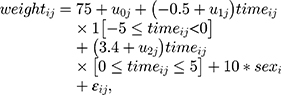
Centring each patient’s follow-up time (in weeks) at their treatment initiation, we fitted the following mixed model to these data [Equation 1]:

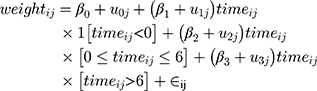
where i denotes the follow-up time and j denotes the patient, and 1[] is an indicator for the event in square brackets. We then fitted the same model adjusting for sex, age and smoking at treatment initiation (as fixed effects). These mixed intercept and slope models were fitted by Restricted Maximum Likelihood, and hereafter we call them just mixed-effects models (MEM).

We also fitted an ‘aggregate-level’ SR model by averaging available weight records at each time point (across-individuals average), and then fitting the standard regression version of [Equation 1] – ie, omitting the person-specific random effects-. Because this model is fitted to data aggregated over individuals, no adjustment for sex, age or smoking was possible.

Finally, we fitted a similar model, but now weighting by the inverse of the number of bodyweight values observed at each time point. We called this model the ‘aggregate-level’ SR-W1, which may help to improve standard errors by including a more accurate sample size information at each time-point.

These models were used to examine the issues arising from the ‘aggregate-level’ SR analysis when outcome (weight measurements) data are missing, which was part of our first study objective.

Imposed Missing Data and Second Analysis

For our second objective, we wanted to explore the issues arising from covariate data missing at treatment initiation. Therefore, we intentionally set smoking records MAR on sex, and increased the amount of missing data on weight MAR on sex, to explore later the potential differences between estimates from complete case analysis (removing cases with smoking missing) and MMI (preserving those cases and imputing smoking). This controlled missing data generation scenario was used evaluate all analysis methods: ‘aggregate-level’ SR, ‘aggregate-level’ SR-W1, MEM, and MMI followed by a mixed-effects model (MI-JOMO with MEM).

In detail, we set weight values MAR dependent on sex and time from treatment initiation, so that a fraction of observed data was similar to that shown in Figure 1. In addition, we set smoking MAR on sex, randomly removing 80% of records from men and 20% from women. Both missing mechanisms are described in detail in Appendix A.

In our subsequent analyses, we first fitted the same MEM [Equation 1] to the incomplete data, adjusting for covariates (complete case analysis). Then, we used a substantive-model-compatible joint-modelling multilevel multiple imputation (MI-JOMO)²¹ to impute the missing smoking values and fitted the same substantive model (MEM adjusted) to each imputed data set and combined the results using Rubin’s rules. We generated 20 imputed datasets with MI-JOMO, and we used a burn-in of 1000 iterations and then further 1000 iterations between each imputation. We name this model MI-JOMO with MEM.

Lastly, we fitted the ‘aggregate-level’ SR and ‘aggregate-level’ SR-W1 models. Full details and codes for all models are given in Appendix A.

Results

Overall, there were 6522 individuals with at least one weight measurement and complete age, sex or smoking status data. Of these, 2954 (45.3%) were men and 3568 (54.7%) were women. On average, there were 4.8 (sd 5.5) weight records per person over the observation period. Individuals were aged 50.2 (sd 18.9) years on average, and 2658 (40.8%) reported being current smokers.

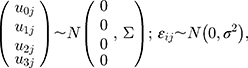
There were substantial differences between estimates derived from MEM and SR (Table 1, section ‘THIN: Data Fully Observed’). For example, the short-term weight change (beta2) was 0.462kg/week from MEM (adjusted) and 0.816kg/week and 0.807kg/week from SR and SR-W1, respectively. Likewise, pre-treatment and long-term periods, weight change rates from SR and SR-W1 were more than double the MEM estimates. In general, all estimates of weight change from SR analyses were higher in magnitude than those from MEM, which also implies a more substantial ITS treatment effect.

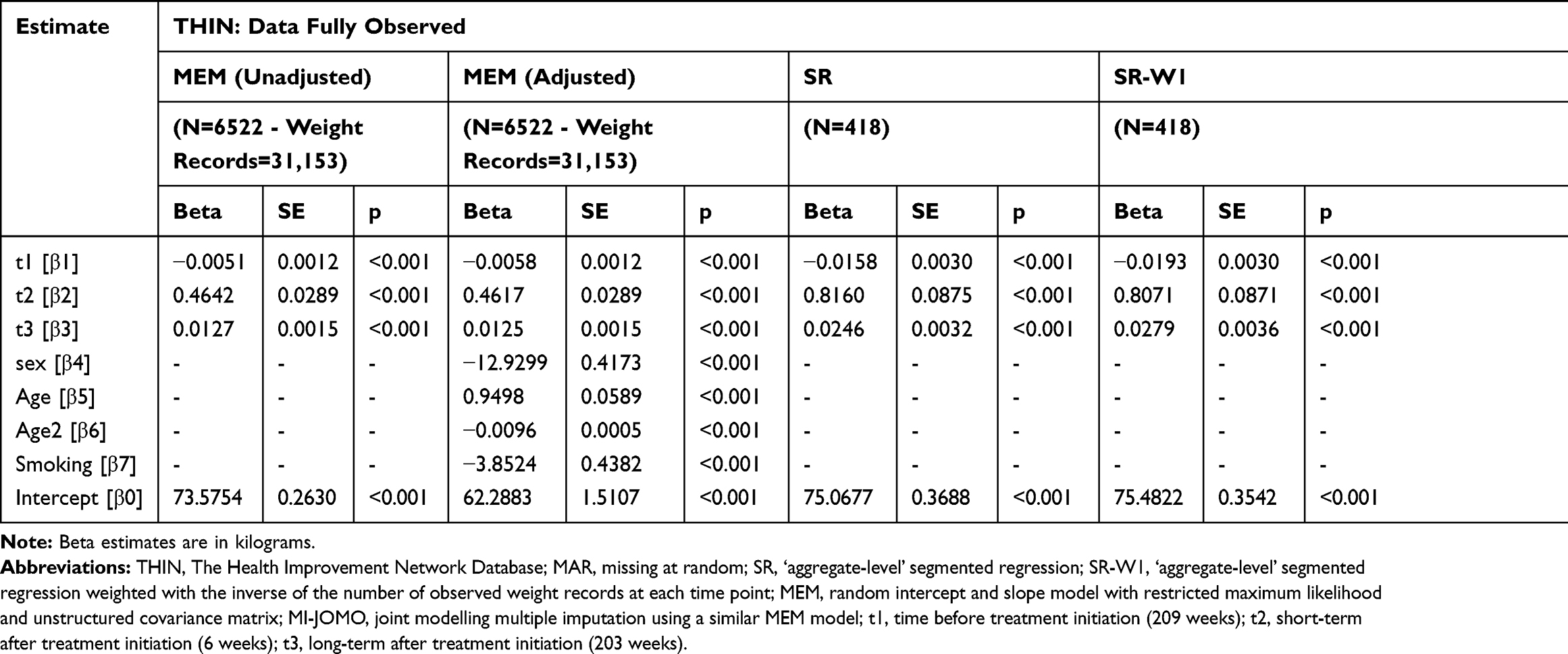Table 1 Estimated Weight Change Over Time Before and After Olanzapine Treatment Initiation from the Example in Section 2, Which Also Describes the Various Analysis Methods

After further removal of weight records, 6181 individuals remained with one or more weight records. There were 4.3 (sd 5.3) average weight records per person over the observation period. The average age was 50.6 (sd 19) years, and 2613 (42.3%) were men. After removal of smoking records at baseline there were only 3379 individuals with a record of their smoking status and 1188 (35.2%) of them were current smokers.

In general, estimates from MEM with and without MI-JOMO were similar for pre-treatment and long-term effects, and both close to those estimated under MEM with full data. However, the MI-JOMO with MEM for short-term were closest to those estimated under MEM with full data (Table 1). ITS estimates from SR differed substantially from the estimates from MEM with and without MI-JOMO (Table 1, Figure 2), with SRs reporting a weight pre-treatment (beta1) and long-term trajectories (beta3) closer to zero. For SR-W1, the long-term treatment effect was similar to the MEM estimates, while the short-term effects estimates (beta2) were much higher than MEM estimates. For both the SR and SR-W1 models, pre-treatment and long-term effects were also different when fitted to data with and without imposed missing values.

Figure 2 Estimated weight trajectories before and after initiation of olanzapine treatment, from the data in Section 2 (motivating example). Circles are weight averages at each time point, dashed line – SR model fitted to these averages; solid line – model [Equation 1] fitted to the raw data by MEM.

The immediate treatment effect, estimated as the difference between the negative and positive trajectories before and after olanzapine initiation, was highest for the SR approach (Table 1 and Figure 2). For example, the SR-W1 method suggested a cumulative short-term weight gain of 4.72kg, a long term of 2.13kg, and a total of 6.85kg. In contrast, the estimates based on MEM with MI-JOMO (short-term=2.47kg, long term=2.46kg, total=4.93kg) and without MI-JOMO (short-term=2.75kg, long term=2.70kg, total=5.45kg) were less for the short term and the total accumulated (see 95% CI in Appendix B).

In summary, individual-data models such as MEM [Equation 1] produced notably different results from SR models with ‘aggregate-level’ data. Further, if covariate values are MAR, use of MI-JOMO can recover information by bringing individuals with these missing covariates back into the analysis, avoiding potential bias and increasing precision. By contrast, the often-used SR ‘aggregate-level’ analysis cannot adjust for covariates and appears to be biased when weight data are MAR (depending on time and covariates). This may often be the case when analysing health-care records.

Simulation Study

We now report the results of a simulation study, based on the motivating clinical example and designed to evaluate the performance of SR and MEM (with and without MMI) under controlled conditions. We are adding to this evaluation another method called Prais-Winsten regression, which is similar to SR but is recommended by ITS guidelines to account for autocorrelation at the aggregate level.¹ In particular, we wish to determine whether the differences between the various analysis methods are due to the way they handle missing data.

Simulation Design

Study Model

For the simulation study, we designed an ITS dataset where the treatment of interest was the initiation of antipsychotic treatment, and we examined change in body weight (in kilograms) over time. The covariates were sex, age (years) and smoking status (yes/no), measured at initiation of treatment. The ITS impact model⁸ is a linear weight trajectory whose slope changes only once – at treatment initiation – ie, slightly simpler than our previous example. We included five time-units before and five after treatment initiation. We modelled the evolution of weight over time using two continuous linear splines, jointing at treatment initiation.

Data Generation

Each simulated dataset with 1000 observations was generated as follows:

1. Sex was generated as a random variable from a Bernoulli distribution with probability 0.5.
2. For each individual, weight observation times were fixed at the same 11 equally spaced times between −5 and +5, ie, centred at treatment initiation, which is at time 0.
3. Weight was generated from the following random intercept and slopes model [Equation 2]:

   

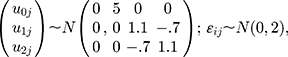
where i denotes the follow-up time and j denotes the patient, and 1[] is an indicator for the event in square brackets. We referred to this as ‘Data Generation Mechanism Base’ (DGM-base). We also generated data from DGM-extended covariates [Equation 3]:

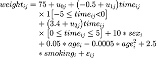
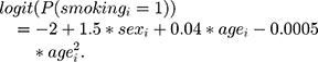
Age was generated as a random variable from a normal distribution with mean 45 and sd 10. Smoking was binary and generated as follows:

Having generated the full data, we made observations missing using two missing data mechanisms:

1. MAR-1: starting with the fully observed weight variable at treatment initiation (), pre- and post-treatment initiation values of weight at times were set to missing () dependent on the individual’s sex. For the missing sequence, pre-treatment setting of missing values was reverse-sequential () and post-treatment setting was forward-sequential (). For both directions () of MAR-1 mechanism, we defined the probability of being missing by: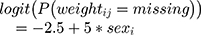shaping the patterns of missing weight data and setting more weight records being observed for women than men. Both patterns and proportion of missing values are available in Appendix C. MAR-1 was applied on data generated under DGM-base only.
2. MAR-2: similar to MAR-1, but now the probability of weight being missing also depends on the individual’s random intercept, age and smoking. As the random intercept is unobservable (as smoking will partially be), this mechanism is a mix between MAR and MNAR (missing not at random). Moving away from treatment initiation (in both directions), the probability of weight being missing is monotonically given by:

   

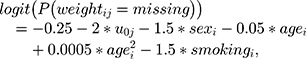
where −0.25 helped to shape the overall proportion of missing data over time; -1.5 set more weight records to be observed for men (only for explicative purposes); −2 set more weight records to be observed for individuals who are heavier at treatment initiation; −0.05 and 0.0005 set more missing data for younger individuals, and −1.5 set more weight records to be observed for smokers. We also set about 30% of smoking values to be missing with probability:

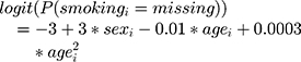
MAR-2 was applied to data from DGM-extended-covariates only. For both described mechanisms (MAR-1 and MAR−2), the proportion of missing weight data in the simulated sample was set to approximately 60% of individuals. In the other 40% of the data, we set only one weight record per individual at any time point, setting more individuals with only one weight record at treatment initiation (MAR dependent on the treatment initiation). This additional mechanism sought to emulate the missing data proportions and patterns seen in the clinical data used for the illustrative example (see Appendix C).

We simulated 1000 full datasets for each of the two scenarios, and then applied the missing data mechanisms to obtain the partially observed data.

Analysis Methods Evaluated

We analysed the full and partially observed data using each of the following six methods (see summary in Appendix D):

1. SR: this averaged observed individual weight measures at each time point and then fits a linear regression on time (maximum likelihood estimator), with a knot at zero.
2. SR-W1: (weighted SR version 1) similar to SR but weighted by the inverse of the number of observed weight records at each time point.
3. SR-W2: (weighted SR version 2) similar to SR-W1 but the number of observed weight records – used for weighting – were counted at each time point by sex and age. We categorised age using its quartiles (before averaging). When smoking data were incomplete, smoking was not included as a covariate for SR-W2.
4. Prais-Winsten: regression similar to SR but adjusted for serial correlation at the aggregate level by assuming errors that follow a first-order autoregressive process,²² an approach typically used in ITS analysis for controlling the autocorrelation issue.¹
5. MEM: we fitted the data generating model [Equations 2 and 3] using Restricted Maximum Likelihood with an unstructured covariance matrix for the random effects.
6. MI-JOMO (with MEM): We first imputed the missing covariate values, using multilevel substantive-model-compatible joint modelling multiple imputation, with the JOMO package in R. As described in^23,24 this imputes missing values consistent with the substantive model [Equation 1]. It does this by factorising the joint model into a joint model for the covariates and a conditional model for the outcome given the covariates. Then, the estimation and imputation process allows compatibility between the imputation and analysis models (MEM in this case), even with longitudinal data.²⁴ We used 5 imputations and 1000 iterations (before the first, and between each subsequent imputation) to impute the missing covariate smoking status. We did not impute the missing weight, as (in the absence of auxiliary variables) no information can be recovered by doing this. Note that standard fully conditional specification²⁵ is not evaluated because it is inappropriate for handling the irregular observation times we expect in real longitudinal data. We only used MI-JOMO in the MAR-2 scenario.

Estimands and Performance Measures

We focused on the slope estimates (true values: and ) from all methods evaluated in both MAR scenarios (MAR-1 and MAR-2), by examining the bias, empirical standard error, model-based standard error and confidence interval coverage.²⁶

Simulation Results

In the first scenario (DGM-base), all SR methods were biased except from when data were fully observed (Table 2). However, the coverage of these methods was low (<61%) due to their small model-based standard errors, even the weighted methods (SR-W1 and SR-W2) and the method adjusted for serial correlation (Prais-Winsten). Conversely, MEM provided reasonably good coverage for and (>94%) for unbiased estimates.

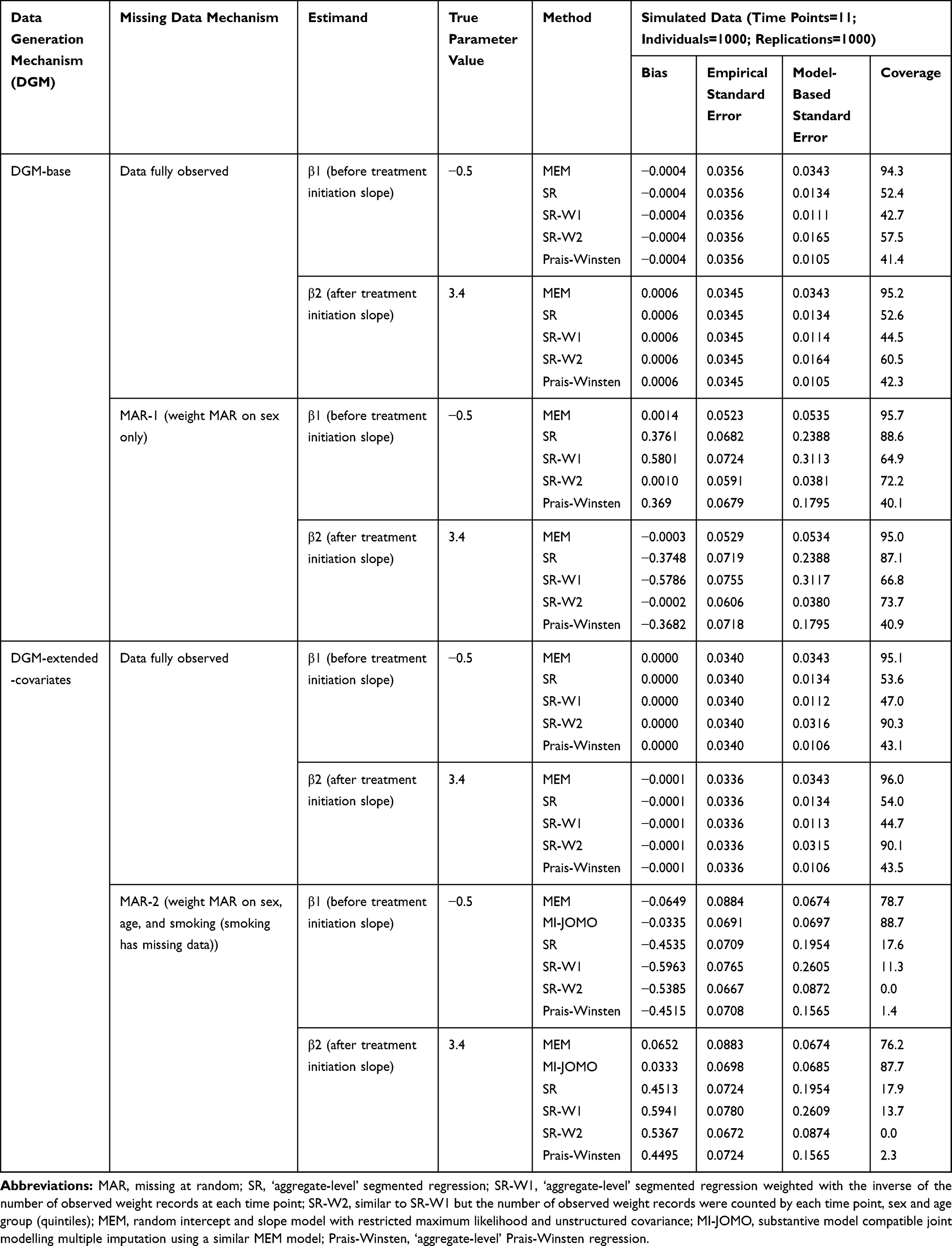Table 2 Simulation Results

Where weight was missing based on sex only (MAR-1), MEM showed unbiased results and the best coverage (≥95%). SR and SR-W1 produced biased estimates for both pre- and post-treatment initiation slopes, showing the highest model-based standard errors. Because the missingness mechanism depended on sex, and women weighed less than men, the preliminary data aggregation step in SR and SR-W1 biased the estimated slopes (see example in Figure 3, MAR-1). The SR bias was corrected using inverse-probability weights based on sex (SR-W2), but coverage was low (<74%) due to too-small model-based standard errors. The Prais-Winsten model was not successful in correcting the SR bias since it does not incorporate information on missing data at the individual-level as SR-W2 does.

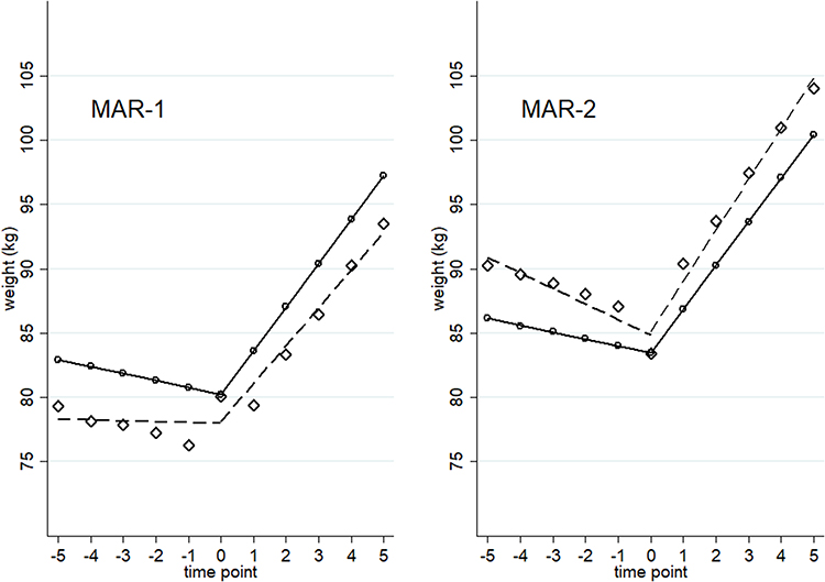Figure 3 Weight trajectories from a simulated dataset in which weight is fully observed (circles and solid lines) or missing at random (diamonds and dashed lines).

In the second scenario (DGM-extended-covariates), with full data, all methods were unbiased (Table 2). MEM provided the best coverage for and (>95%), followed by SR-W2 (>90%). Although with unbiased estimates, SR, SR-W1 and Prais-Winsten provided a low coverage (<55%) due to their small model-based standard errors. SR, SR-W1 or Prais-Winsten cannot provide different averages by sex and age at each time point, which can be provided by SR-W2. Having more variability at each time point produced higher – and more realistic – standard errors from SR-W2.

On the other hand, with missing values in weight and smoking status (MAR-2), MI-JOMO had the best performance. MEM showed poorer performance after all covariates were included in the imputation and study models and there were missing smoking data, producing slightly biased estimates and low coverage (<79%). In the same scenario, MI-JOMO performed better than MEM, providing less biased estimates, closer values of empirical and model-based standard errors, and higher coverage (>87%). For both methods, we should consider that there is some residual bias because of the dependence of observation of weights on the random intercepts. While the results in the bottom half of Table 2 show this resulted in a bias in the MI-JOMO analysis, this was not severe, and the resulting inferences were still usable. Conversely, SR, SR-W1, SR-W-2 and Prais-Winsten performed extremely poorly, showing large bias and low coverage (<18%).

The ‘aggregate-level’ SR analysis biased the slope trajectories in different directions, which we illustrated by our simulations (Figure 3).

Discussion

ITS provides a conceptually attractive approach for assessing the impact of treatments because each individual acts as their own control. However, its innate strength, leading to its increasing use,⁴ raises important questions about how to appropriately handle missing data. As our example illustrates, incomplete outcome data (in our case, weight) is an intrinsic feature of this kind of study because the underlying observational data do not follow any pre-planned schedule. This means that, at any specific time, the marginal distribution of the response is unlikely to be representative of the underlying population.

The results of our studies demonstrate that the ‘aggregate-level’ approach will generally be biased when individual-level data are missing at random (MAR). Indeed, the motivating example shows this bias could lead to a substantial exaggeration of the actual effect of the studied intervention. In the example, the difference between pre- and immediate post-treatment weight change (biased slopes) increases the overall effect attributed to olanzapine. However, it is not always possible to determine the direction of bias. This is because the direction of the average-points bias depends on how the covariate is associated with the missingness of weight records. Even when the ‘aggregate-level’ SR analysis does not bring about a bias issue, our results highlight that the precision is inaccurate as the standard errors for this method are typically grossly underestimated.

When data are missing-at-random at the individual level, averaging before SR means that data are missing-not-at-random (MNAR) at the cluster level. This leads to the bias observed for the ‘aggregate-level’ SR analysis. For example, in the MAR-1 mechanism, ‘aggregate-level’ SR analysis loses the information about the distribution of weight records that are MAR on sex at each time point, due to the averaging-step. Thus, sex becomes unobservable at the ‘aggregate-level’, making weight records MNAR on sex at this level and biasing the subsequent analysis using those averages. As we demonstrate in the same simulation study, this issue could be handled by including sex in the averaging-step (SR-W2). However, in practice, any version of SR-W2 will be hard to apply since other covariates are typically incomplete as well.

A natural alternative to the ‘aggregate-level’ analysis is to model the individual patient data explicitly. When the reason for outcome data being observed depends principally on time (eg, before and after treatment initiation), underlying patient characteristics (eg, sex, age) and observed outcomes (eg, observed weights), the unseen values are plausibly MAR. In this setting, our simulation results demonstrate that a carefully formulated longitudinal model provides a practical approach for improved inference.

Longitudinal models should be formulated carefully to include covariates predictive of both the outcome and the chance of observing it, which are key for avoiding bias. Where it is not desired – or appropriate – to include some such variables in the substantive analysis, an MMI approach should be considered, where these variables are included as auxiliary variables. Care should also be taken to model the longitudinal correlation of the outcome appropriately, as this is particularly important for missing data, as well as to use the observed rather than expected information for likelihood-based models. In particular, having random intercepts alone, or having uncorrelated random intercepts and slopes, should be avoided (see Appendix E for other practical suggestions).²¹ If data at the individual level are not available, and the researcher suspects that a strong MAR mechanism affect the outcome points over time (eg, averages or rates), the issue should be stated as a limitation as recommended in reporting guidelines.^27,28

Our results show that MMI provides a practical approach for handling missing covariates in the analysis. When performing MMI, it is essential to both use an approach that properly takes account of the multilevel structure, and uses an approach that is compatible with the substantive model (which here includes splines for the effect of time). The JOMO package in R has the flexibility to do both.

We set our example and simulations with averages of a continuous variable, but a similar problem can happen with other types of outcomes. Rates (proportions), another common ITS outcome,⁵ can also be biased when outcome data are MAR at the individual level. For example, if the numerator of the rate (the events) is higher in women than men, and the missingness process generates more missing records for women, the rate will be underestimated at the ‘aggregated-level’ (eg, at time points, hospitals or districts). The ITS analysis will use those rates as consecutive points, biasing the estimated trajectories. Similar reasoning can be applied to binary and count ITS outcomes. Even using other recommended analysis methods than SR, such as ARIMA models,¹ the bias problem will remain in the ‘aggregate-level’ used for the time series. Although we did not formally evaluate these alternative methods, some reflections can be enlightened by the study findings. In the aggregate-level approach, ARIMA models will be fitted after the averaging-step; therefore, the ITS will be based on population-level average points already biased. Other options useful for individual-level data, such as generalised estimated equations (GEE) can be applicable. However, because they are moment-based estimates, precisely like the aggregate data analysis, its estimates will be biased unless data are missing completely at random.^29,30

This is the first time that this averaging-step problem for MAR data has been studied with simulations and real data. Our results will help to guide future ITS studies. We focused our study on the situation when data are missing at random. However, we are aware there may be other scenarios where data missing not at random (MNAR) could bias estimates. For example, if weight is only recorded for those with a high or low weight. This scenario goes beyond the scope of this study but in practice, when a strong MNAR mechanism is suspected, a sensitivity analysis is possible using a pattern mixture approach.^31,32

In conclusion, the segmented regression using averaged data points can over or underestimate the effect evaluated in interrupted time series analyses, when performed on outcome data missing at random at the individual level. However, such a problem can be addressed by using mixed models. If there are also covariates missing at random, mixed models can be combined with multilevel multiple imputation and provide unbiased results.

References

1. Lopez Bernal J, Cummins S, Gasparrini A. Interrupted time series regression for the evaluation of public health interventions: a tutorial. Int J Epidemiol. 2017;46(1):348–355.
2. Myer AJ, Belisle L. Highs and lows: an interrupted time-series evaluation of the impact of North America’s only supervised injection facility on crime. J Drug Issues. 2018;48(1):36–49. doi:10.1177/0022042617727513
3. Ejlerskov KT, Sharp SJ, Stead M, Adamson AJ, White M, Adams J. Supermarket policies on less-healthy food at checkouts: natural experimental evaluation using interrupted time series analyses of purchases. Popkin BMed. PloS Med. 2018;15(12):e1002712. doi:10.1371/journal.pmed.1002712
4. Jandoc R, Burden AM, Mamdani M, Lévesque LE, Cadarette SM. Interrupted time series analysis in drug utilization research is increasing: systematic review and recommendations. J Clin Epidemiol. 2015;68(8):950–956. doi:10.1016/J.JCLINEPI.2014.12.018
5. Hudson J, Fielding S, Ramsay CR. Methodology and reporting characteristics of studies using interrupted time series design in healthcare. BMC Med Res Methodol. 2019;19(1):137. doi:10.1186/s12874-019-0777-x
6. Kontopantelis E, Doran T, Springate DA, Buchan I, Reeves D. Regression based quasi-experimental approach when randomisation is not an option: interrupted time series analysis. BMJ. 2015;350(jun09 5):h2750. doi:10.1136/bmj.h2750
7. Lopez Bernal J, Cummins S, Gasparrini A. The use of controls in interrupted time series studies of public health interventions. Int J Epidemiol. 2018;47(6):2082–2093. doi:10.1093/ije/dyy135
8. Lopez Bernal J, Soumerai S, Gasparrini A. A methodological framework for model selection in interrupted time series studies. J Clin Epidemiol. 2018;103:82–91. doi:10.1016/J.JCLINEPI.2018.05.026
9. Bao L, Peng R, Wang Y, et al. Significant reduction of antibiotic consumption and patients’ costs after an action plan in China, 2010–2014. Singer AC ed. PLoS One. 2015;10(3):e0118868. doi:10.1371/journal.pone.0118868
10. Yoo KB, Lee SG, Park S, et al. Effects of drug price reduction and prescribing restrictions on expenditures and utilisation of antihypertensive drugs in Korea. BMJ Open. 2015;5(7):e006940. doi:10.1136/bmjopen-2014-006940
11. Uijtendaal EV, Zwart-van Rijkom JEF, de Lange DW, Lalmohamed A, van Solinge WW, Egberts TCG. Influence of a strict glucose protocol on serum potassium and glucose concentrations and their association with mortality in intensive care patients. Crit Care. 2015;19(1):270. doi:10.1186/s13054-015-0959-9
12. Petersen I, Welch CA, Nazareth I, et al. Health indicator recording in UK primary care electronic health records: key implications for handling missing data. Clin Epidemiol. 2019;11:157–167. doi:10.2147/CLEP.S191437
13. Rabe-Hesketh S, Skrondal A, Skrondal A. Multilevel and Longitudinal Modeling Using Stata. Stata Press Publication; 2008. Available from: https://books.google.co.uk/books?hl=en&id=woi7AheOWSkC&oi=fnd&pg=PR21&dq=Multilevel+and+Longitudinal+Modeling+Using+Stata+second+edition&ots=edLw2c_PUz&sig=Hw_YmlcM7lcKV5k00uYt6WKjz5A#v=onepage&q=MultilevelandLongitudinalModelingUsingStatasecondedition&f=false.
14. Pedersen AB, Mikkelsen EM, Cronin-Fenton D, et al. Missing data and multiple imputation in clinical epidemiological research. Clin Epidemiol. 2017;9:157–166. doi:10.2147/CLEP.S129785
15. Roland M, Guthrie B, Thomé DC. Primary medical care in the United Kingdom. J Am Board Fam Med. 2012;25(Suppl 1):S6–S11. doi:10.3122/jabfm.2012.02.110200
16. Blak B, Thompson M, Dattani H, Bourke A. Generalisability of The Health Improvement Network (THIN) database: demographics, chronic disease prevalence and mortality rates. J Innov Health Informatics. 2011;19(4):251–255. doi:10.14236/jhi.v19i4.820
17. Horsfall L, Walters K, Petersen I. Identifying periods of acceptable computer usage in primary care research databases. Pharmacoepidemiol Drug Saf. 2013;22(1):64–69. doi:10.1002/pds.3368
18. Maguire A, Blak BT, Thompson M. The importance of defining periods of complete mortality reporting for research using automated data from primary care. Pharmacoepidemiol Drug Saf. 2009;18(1):76–83. doi:10.1002/pds.1688
19. Bak M, Fransen A, Janssen J, van Os J, Drukker M. Almost all antipsychotics result in weight gain: a meta-analysis. PLoS One. 2014;9(4):e94112.
20. Bazo-Alvarez JC, Morris TP, Carpenter JR, Hayes JF, Petersen I. Effects of long-term antipsychotics treatment on body weight: A population-based cohort study. J Psychopharmacol. 2019;026988111988591. doi:10.1177/0269881119885918
21. Quartagno M, Grund S, Carpenter J. Jomo: A flexible package for two-level joint modelling multiple imputation. R Journal. 2019;11(2):205.
22. Prais SJ, Winsten CB. Trend estimators and serial correlation. Cowles Commission discussion paper Chicago; 1954.
23. Goldstein H, Carpenter JR, Browne WJ. Fitting multilevel multivariate models with missing data in responses and covariates that may include interactions and non-linear terms. J R Stat Soc Ser A (Statistics Soc). 2014;177(2):553–564. doi:10.1111/rssa.12022
24. Quartagno M, Carpenter JR. Multiple imputation for discrete data: evaluation of the joint latent normal model. Biometrical J. 2019;61(4):
25. Van Buuren S. Flexible Imputation of Missing Data. Chapman and Hall/CRC; 2012.
26. Morris TP, White IR, Crowther MJ. Using simulation studies to evaluate statistical methods. Stat Med. 2019;38(11):2074–2102. doi:10.1002/sim.8086
27. von Elm E, Altman DG, Egger M, Pocock SJ, Gøtzsche PC, Vandenbroucke JP. The strengthening the reporting of observational studies in epidemiology (STROBE) statement: guidelines for reporting observational studies. J Clin Epidemiol. 2008;61(4):344–349. doi:10.1016/J.JCLINEPI.2007.11.008
28. Benchimol EI, Smeeth L, Guttmann A, et al. The reporting of studies conducted using observational routinely-collected health data (RECORD) statement. PloS Med. 2015;12(10):e1001885. doi:10.1371/journal.pmed.1001885.
29. Funatogawa I, Funatogawa T. Longitudinal Data Analysis: Autoregressive Linear Mixed Effects Models. Springer; 2018.
30. Copas AJ, Seaman SR. Bias from the use of generalized estimating equations to analyze incomplete longitudinal binary data. J Appl Stat. 2010;37(6):911–922. doi:10.1080/02664760902939604
31. Carpenter JR, Kenward MG. Multiple Imputation and Its Application. John Wiley & Sons; 2013. https://www.wiley.com/en-us/Multiple+Imputation+and+its+Application+-p-9780470740521.
32. Cro S, Carpenter JR, Kenward MG. Information-anchored sensitivity analysis: theory and application. J R Stat Soc Ser A (Statistics Soc). 2019;182(2):623–645. doi:10.1111/rssa.12423
© 2020 The Author(s). This work is published and licensed by Dove Medical Press Limited. The
full terms of this license are available at https://www.dovepress.com/terms
and incorporate the Creative Commons Attribution
- Non Commercial (unported, 3.0) License.
By accessing the work you hereby accept the Terms. Non-commercial uses of the work are permitted
without any further permission from Dove Medical Press Limited, provided the work is properly
attributed. For permission for commercial use of this work, please see paragraphs 4.2 and 5 of our Terms.