Glaucoma Diagnosis Through the Integration of Optical Coherence Tomography/Angiography and Machine Learning Diagnostic Models

Introduction

Glaucoma is the second leading cause of blindness worldwide.¹ Primary open angle glaucoma (POAG), the most common variety, is defined as a progressive neurodegenerative disease of the retinal ganglion cells with characteristic features of the optic disc, usually accompanied by corresponding visual field (VF) defects, with or without elevated intraocular pressure (IOP).² Although the exact etiology is still poorly understood, the most prevalent theories pertain to elevated IOP (mechanical), inherent poor blood flow to the optic nerve (vascular), or a combination of both.³ Multifactorial risk factors for glaucoma include increasing age, elevated IOP, Black race, family history, myopia, and diabetes (DM).²

The diagnosis of glaucoma and its progression are based on three inconsistent, variable, and inherently subjective methods: measurement of IOP, evaluation of optic nerve, and VF testing. IOP measurement depends on the central corneal thickness (CCT), type of instrument used, skill of the examiner, and time of day.^2,4 Accurate examination of the optic nerve is challenging with both inter- and intra-examiner variations.⁵ The VF exam has the most subjective bias with well-known short-term and long-term fluctuations.⁶

Optical coherence tomography angiography (OCTA) ushered in a first attempt to objectively measure both structural and vascular components of the optic nerve and retina.⁷ However, a major obstacle for the use of OCTA is the interpretation of over 30 structural, volumetric numerical measures characterizing the optic nerve and retina of each eye upon scanning. This deluge of raw data presents a significant challenge for clinicians to accurately characterize normal from at-risk glaucoma patients. In addition, there is a lack of information on normative values for optical coherence tomography (OCT)/OCTA parameters, or quantifiable “ground truth”, which contributes to the challenges in managing glaucoma. Artificial intelligence (AI) has the potential to analyze “big data” and thus accelerate the speed and scale of clinical diagnosis and reduce reader bias in the analysis of clinical data.

Recently, machine learning (ML), a subset of AI, emerged as a powerful tool within the field of ophthalmology, and more specifically glaucoma. It can produce predictive diagnostic models directly from sample data. Early work included diagnoses from fundus photography and VF data, while more recent work includes diagnoses from OCT.^8,9 In 2019, Chan et al reported the first use of ML to detect glaucoma using OCTA disc and macular images.¹⁰ This work used a much smaller dataset than the work discussed herein and achieved an accuracy of 94.3% using six features from the disc images.

The aims of our study were two-fold. First, to characterize OCT/A parameter ranges for healthy eyes (HE) and those with various stages of glaucoma, and second, to develop ML algorithm based clinical decision support tool to aid classification of glaucomatous eyes (GE). We hypothesized that ML and OCT/A data can help clinicians distinguish between normal vs glaucomatous patients and distinguish between mild, moderate, and severe glaucoma.

Materials and Methods

Data Source and Participants

The data in this retrospective study were obtained from electronic medical records of 887 patients seen in the Glaucoma Clinic at the University of Texas Southwestern Medical Center (UTSW) from January 2017 through July 2019. Institutional Review Board approval was obtained from UTSW, and we followed the tenets of the Declaration of Helsinki and Health Insurance Portability and Accountability Act. The IRB did not require signed consent as there was no direct interaction with patients.

Study inclusion criteria were defined as follows: available OCTA data for at least one eye, age over 18 years, diagnosis of POAG, ocular hypertension (OHT), or no glaucoma, and vision better than 20/200. Subjects are excluded if they have: secondary glaucoma, angle closure glaucoma, retinal or vascular pathology, non-glaucomatous optic nerve damage, incomplete OCTA scans or OCTA with poor image quality, as defined by a signal strength index (SSI) ≥45 for macula and ≥35 for optic nerve imaging.

Of the 1683 eyes from 887 subjects initially selected, 312 (18.5%) eyes were subsequently excluded secondary to incomplete or poor quality OCTA scans. Figure 1 illustrates the process of eye selection. The data collected included: age, sex, race, family history of glaucoma, hypertension, diabetes, IOP, CCT, refractive error prior to any surgical correction, and full OCT/A parameters. Family history of glaucoma was self-reported and defined as a first- or second-degree relative with glaucoma. History of hypertension (HTN) and DM was also self-reported or obtained from the problem list in the patient’s chart. Precise definitions of a history of myopia, hypertension, diabetes, and glaucoma are provided in Supplementary Table S1.

Figure 1 Consort flow diagram. Notes: This flow chart illustrates the inclusion and exclusion criteria selecting eyes for this study as well as the number of eyes included at each step.

The eyes from each subject were individually diagnosed as follows. HE were defined as those with IOP less than 21 mmHg, normal optic nerve and VF appearance. Some patients were referred by optometrists due to a single elevated pressure or suspicious optic discs. After undergoing full ophthalmological examination, including fundus exam, IOP, and OCTA, if they were deemed to be healthy, they were subjected to a second round of testing within 6 months before being defined as HE. Eyes with OHT (suspect) had IOP ≥21 mmHg at diagnosis but normal optic nerve and VF. Eyes with POAG had characteristic optic disc (vertical cupping, notching, thin neuroretinal rim, disc hemorrhage), open iridocorneal angles confirmed by gonioscopy, and characteristic VF defects with or without elevated IOP. Eyes with POAG were further classified into mild, moderate, or severe glaucoma based on their VF mean deviation of <–6 dB, between −6 dB and −12 dB, and worse than −12 dB, respectively, using the modified Hodapp–Parrish–Anderson classification.¹¹ Lag time between VF results and glaucoma severity classification was within 6 months. KSK and GAH verified each chart to confirm the diagnosis.

Imaging data were gathered using the Optovue AvantiXR AngioVueHD scanner (Optovue^®, Freemont, CA, USA). This scanner combines OCT/A imaging in a single system. Parameters were derived by the AngioAnalytics software (Version 2018.0.0.18) with images of the retina and optic nerve obtained on the same day by a trained ophthalmology imaging technician. The study used scans measuring 3 mm×3 mm on retina and 4.5 mm×4.5 mm on optic nerve. OCT/A results were used for both the structural and vascular parameters of the optic nerve head and the retina. Data were recorded and stored as a REDCap database (developed at Vanderbilt University, Nashville, TN, USA) on a UTSW server.

From the OCT/A, clinical and demographic patient data, KSK and GAH initially identified 98 clinically relevant features. These were culled by weighing the clinical importance of these against the amount of missing data for each feature, resulting in a total of 64 features including 6 clinical, 3 demographic, and 54 OCT/A as listed in Supplementary Table S2. The ML approaches explored in this study do not inherently handle missing data, therefore eyes with any missing features were removed. The final dataset consisted of the 64 features for 1371 eyes classified as 462 HE and 909 glaucomatous eyes (GE) (377 OHT, 160 mild, 156 moderate, 216 severe) from 735 subjects.

Statistical Analysis

Continuous variables were assessed for normality both quantitatively via the Shapiro–Wilk test and qualitatively via histogram and normal probability plots (Supplementary Figure S1-1–S1-4). For non-normal continuous variables, the median and interquartile range were calculated, and the Kruskal–Wallis was used to test significance. For normal continuous variables, the mean and standard deviation were calculated, and one-way ANOVA was used to test significance. For categorical variables, the frequency and percentage of each group were calculated, and chi-square was used. An RxC chi-square test was used to test race. Due to counts of less than 5 per glaucoma severity, other (n=8) and unknown (n=4) race categories were excluded when performing the test. For both the summary statistics as well as the OCT/A parameters, the Bonferroni correction method was applied to adjust significance level as a result of performing multiple tests. Significance level was set at 0.05. Analyses were conducted with Python (Version 3.7.4) and the summary statistics package (Table 1).¹²

Table 1 Demographic and Baseline Characteristics of Study Population

Machine Learning Methods

Machine Learning

ML is the intersection between computer science and statistics. In the ML subspecialty known as supervised learning, tools or models map predictors into targets that generalize well to unseen data, such as data subsequently encountered in a clinic. In this study, the predictors are the combination of demographic, clinical, and OCT/A derived measures, while the targets are the ophthalmologists’ diagnosis per eye. The ML algorithm is the form of the mapping between predictor and target. Unlike statistics, in ML there is no one algorithm that one can select a priori from the data. Consequently, this study compared a judicious selection of representative algorithms from a comprehensive set of ML classifier types that historically performed well across other classification tasks. Our focus in this section was to utilize hand-engineered OCT/A predictors provided by the OCTA machine to predict each eye’s glaucoma diagnosis.

Through supervised training, the model learned a function to predict the clinical diagnosis per eye. Data preparation (Data Preparation) ensured predictors had equal chance of being used in the learned model. Data partitioning (Data Partitioning) was employed to divide the eye samples into disjoint sets including the training, validation, and held-out test sets, while keeping eyes from the same subject in one set. This allowed the models to be trained, optimized, and tested on non-overlapping subsets of the data and enabled the computation of classification performance metrics.

Predictive Model

Classifiers were developed for two use cases: 1) to distinguish HE from GE; and 2) to distinguish HE vs mild glaucoma (Mild) vs moderate glaucoma (Moderate) vs severe glaucoma (Severe) eyes.

Data Preparation

Continuous variables were standardized using the z-score transform. This normalization was done per fold to avoid any leakage. For the inner folds, the mean and standard deviation (SD) were calculated on the training data and applied to normalize the validation data. For the outer folds, the mean and SD were calculated on the combined training and validation data and applied to normalize the held-out test data.

Data Partitioning

A rigorous nested stratified, group 5×10 fold cross-validation strategy was applied to partition the data. Thus 20% of the data was held out for test with 10% of the remaining 80% used for validation. Although less frequently employed, nested cross-validation provides one of the most unbiased estimates of model performance.¹³ Group partitioning ensured that data (multiple eyes) from the same subject were assigned to only one partition. Stratification ensured each partition had a similar distribution of diagnosis, age, and sex when compared to the complete dataset (Supplementary Figure S2).

Predictive Model Development and Optimization

The performance of six ML algorithms was compared. These algorithms include: XGBoost,¹⁴ deep feedforward neural networks (DL),¹⁵ decision trees (DT), support vector classifiers (SVC),¹⁶ partial least-squares discriminant analysis (PLSDA), and the random forest (RF).¹⁷ Specifically, XGBoost was chosen as it frequently ranks at the top in ML competitions. PLSDA was selected as it reduces the dimensionality of the data and often performs well when the data reside on or near a lower dimensional hyperplane in feature space. DT, RF, and SVC were selected as they often provide reasonable performance with tabular data and provide readily interpretable models. Finally, DL was used as it often provides state of the art performance on a range of problems.

The performance of an ML algorithm can depend on suitability of the architecture to the specific classification task. The architecture of the models from each ML algorithm category were optimized. The model architecture is characterized by a set of hyperparameters, such as the number of layers in a neural network or the number of trees in an XGBoost model. Since hand tuning of model hyperparameters is highly dependent on the experience of the ML expert, an unbiased random search¹⁸ was used to optimize the hyperparameters of each ML model for each algorithm. For each ML algorithm, 500 configurations of each model were trained with the exception of PLSDA where 50 configurations were trained, as it is limited by the number of optimizable components. For further details, see the supplemental material including a description of the search space dimensions for all models in Supplementary Table S3.

For each of the six model categories, a winning model configuration was selected at the conclusion of the model category search. To achieve this, for each outer fold, the mean validation performance across the inner folds was computed for each model configuration (hyperparameter set) and the configuration with highest mean validation performance was selected for that fold. The winning model was then trained on all training and validation data, and model performance was computed from the held-out test data, not used for training or model selection. For a given ML algorithm category, the overall model performance across outer folds was computed as the average of performance of the winning models. This process was repeated for the six ML algorithm categories and their test set performance is measured using classification accuracy and the F1 score, the harmonic mean of precision and recall.

Model Error Analysis

In general, the model was accurate with overall diagnostic accuracy of 84%. To better understand where the model is amiss classifying, HE vs GE, an error analysis was applied. The error analysis compared the incorrect and correct predictions on the held-out test data, to which the model assigned a high confidence. To determine which characteristics were associated with incorrect predictions, the demographic features were assessed using student’s and chi-squared t-tests.

Results

Baseline Characteristics

Table 1 characterizes the demographic distribution of the dataset. Of note, six subjects were excluded from race calculations as their race information was unavailable. Age (p<0.001) and gender (p=0.043) were both correlated with glaucoma severity, with a female predominance (59.8%). There was a statistically significant difference (p=0.006) between race and glaucoma severity. Of the subjects diagnosed with severe glaucoma, 36.6% of subjects were Black compared to 9.7% who were Asian. In comparison, Black subjects comprised 26.4% of subjects with non-glaucomatous eyes compared with Asian subjects who comprised 19.7%. Neither a comorbidity of diabetes (p=0.483) nor a family history of glaucoma (p=0.666) was associated with glaucoma severity. However, IOP (p=0.048) and a comorbidity of HT (p=0.04) were both significantly associated with glaucoma stage.

OCTA Normative Values

Table 2 provides summary values for 12 clinically significant OCT/OCTA parameters, with an additional 15 shown in Supplementary Table S4. All but two were statistically significant. Foveal avascular zone (FAZ) area and perimeter remained unchanged (p=0.022, p=0.005). On the other hand, average RNFL thickness, eight sector RNFL thickness, and macular full thickness were all inversely related to increasing severity of glaucoma (p<0.001), with greatest differences observed between moderate and severe groups. Similarly, vessel density (VD) percentages for the optic nerve, macula, peripapillary, and inside disc were also inversely related to increasing severity of glaucoma (p<0.001). Rim area significantly decreased (p<0.001) as glaucoma severity increased. Cup-to-disc ratio (CDR) and vertical and horizontal CDR values were unchanged for the control, suspect, and mild groups and showed a marked increase in the moderate and or severe groups (p<0.001).

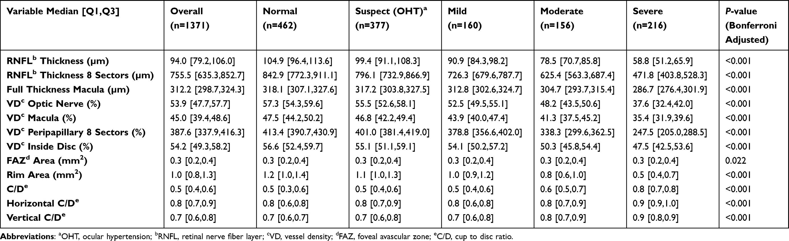Table 2 OCTA Parameters Compared Across Varying Severities of Glaucoma

Machine Learning Classifiers

The performance of the winning ML models was computed using the mean accuracy and the F1 score on the held-out test data (Figure 2). Of the two category models distinguishing HE from GE, all ML algorithms achieved similar accuracy and F1 score performance with the exception of DL. XGBoost provided the highest performance on the held-out test data with an accuracy of 83.9% (chance at 53.5%), an F1 macro score of 83.8%, sensitivity and specificity of 84.2% and 83.5% respectively, and standard deviation of 0.030%. Of the four category classifiers distinguishing HE and three levels of glaucoma, the XGBoost and RF algorithms achieved the highest mean accuracy and F1 score. The XGBoost model again achieved the highest accuracy of 71.3% (chance at 46.5%), F1 macro score of 62.4%, although not statistically different from the performance of the RF, and standard deviation of 0.013%.

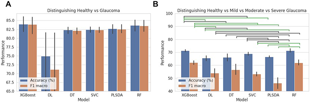Figure 2 Comparison of diagnostic performance across algorithm categories using held-out test data. Abbreviations: DL, deep feed forward neural networks; DT, decision trees; SVC, support vector classifier; PLSDA, partial least-squares discriminant analysis; RF, random forest. Notes: (A) Performance of two category classifiers distinguishing healthy controls vs glaucomatous eyes. (B) Performance of four category classifiers distinguishing controls, and three levels of glaucoma. Significance is colored by the green (t-test p<0.01) and black (p<0.05) bars. Performance measured using overall accuracy (blue) and F1 macro score (orange).

The confusion matrices in Figure 3 show where the models tended to misclassify and provide performance metrics on a per-diagnostic category basis. As both the performance, and confidence in ground-truth classification is highest for the two category XGBoost classifier, both feature importance (Figure 4) and model trees (Figure 5) are presented for this algorithm. These were generated using the XGBoost model that had the lowest generalization error from the outer folds, which was calculated as the absolute difference between the model’s performance on train plus validation data vs its performance on test set data. On the outer fold of the nested k fold cross-validation, the selected, single outer-fold model had an accuracy of 87.6% on the held-out test.

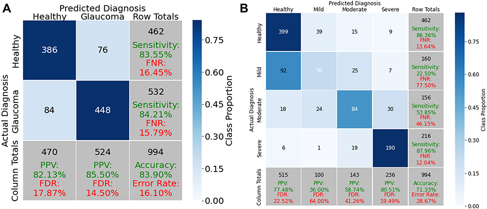Figure 3 Confusion matrices of the proposed XGBoost models using the held-out test data. Abbreviations: FDR, false discovery rate; FNR, false negative rate; PPV, positive predictive value. Notes: (A) Performance for two category classifiers distinguishing healthy controls vs glaucomatous eyes. (B) Performance for four category classifiers distinguishing controls and the three levels of glaucoma.

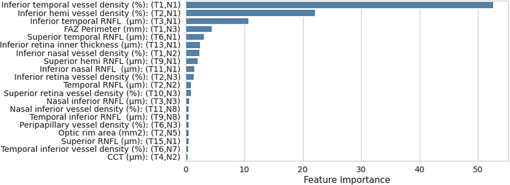Figure 4 Features that distinguish controls from glaucoma, ranked by their importance from the final XGBoost model. Abbreviations: RNFL, retinal nerve fiber layer; FAZ, foveal avascular zone; CCT, central corneal thickness. Notes: Feature importance is calculated as the sum of the product of cover and gain in each node the feature is used weighted by the performance improvement of the tree. For each feature, the importance of each node that uses the feature is summed to provide that feature’s importance. The tree and node where each feature is used is described using notation such as (T1, N1) indicating the feature is used in tree 1, node 1. For brevity each feature lists only its first tree and node.

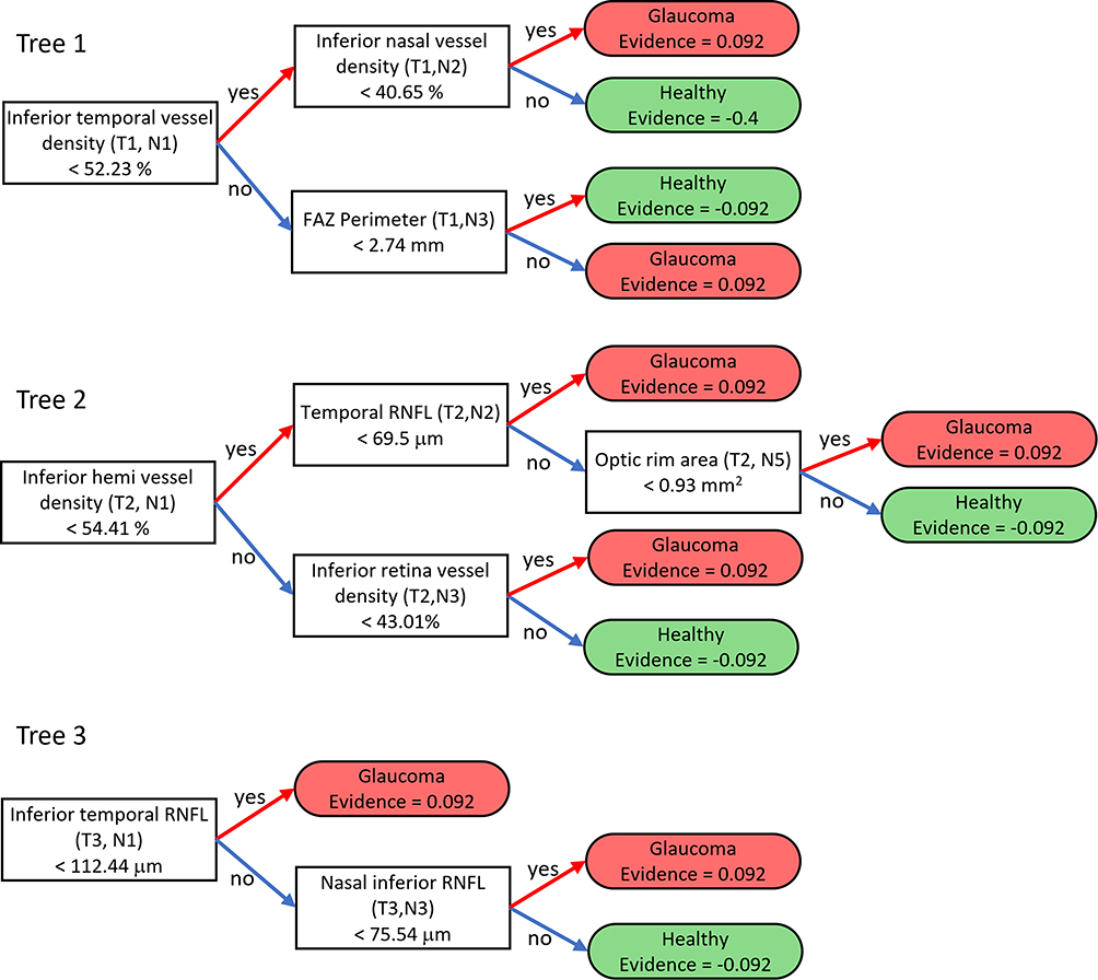Figure 5 The primary (first three) decision trees of the proposed XGBoost model distinguishing controls from glaucoma. Abbreviations: RNFL, retinal nerve fiber layer; FAZ, foveal avascular zone. Notes: To form diagnostic information for a new subject, the subject’s measurement vector is sent through the trees from left to right, in parallel starting at the root nodes. Each decision node routes the sample to one of two child nodes according to a split function that compares a feature to a threshold. This is repeated until the sample arrives at a terminal node which provides class evidence: positive evidence makes glaucoma more likely while negative evidence makes control more likely. The sum of evidence from all trees is transformed into the probability of glaucoma via the sigmoid function. The tree and node number are provided in parentheses.

The first three trees of this model shown in Figure 5 provided a performance of 84.2%. However, to provide a more intuitive method for clinicians to diagnose glaucoma, we also report the single tree generated from our DT algorithm in Figure 6, where an accuracy of 82.3% was achieved, and provide suggested use for the integration of such algorithm results into clinical impression (Supplementary Figure S3).

Figure 6 The decision tree algorithm identified this tree for classifying subjects into healthy vs mild vs moderate vs severe. Abbreviation: RNFL, retinal nerve fiber layer.

Additional models were built including a three-category model to distinguish HE vs suspect vs glaucoma, and four category models that distinguish HE vs suspect vs three stages of glaucoma. These models also performed well above chance accuracy, demonstrating their ability to identify and utilize predictor signal to inform diagnosis, however neither could distinguish HE vs suspect eyes well. Details of the performance of these models are shown in Supplementary Figure S4 and confusion matrices shown in Supplementary Figure S5.

Model Error Analysis

Statistical differences were calculated between the model’s high confidence correct prediction and high confidence incorrect predictions. In Table 3, the 100 most confident correction predictions are compared to the 100 most confident incorrect predictions. Statistically significant differences (p<0.05) in prediction accuracy were observed for myopia (p=0.021), family history of glaucoma (p=0.025), and the presence of HTN (p=0.024). The model was somewhat more accurate for lower myopia (0 to −3 diopters) than at higher myopia (>3 diopters) and this difference was significant. Slightly worse performance was noted if there was no family history of glaucoma or if HTN was present. The model also tended to work better on younger patients. It showed high confidence correctly predicting eyes belonging to subjects with a mean age of 65 years than those from subject with a mean age of 69 years. However, this difference was not statistically significant (p=0.14). Such results suggest that these subpopulations may be more difficult to diagnose unless larger training data are utilized.

Table 3 Error Analysis of the Most Confident 100 Correct Eye Diagnosis Predictions vs the Most Confident 100 Incorrect Eye Diagnosis Predictions

Discussion

In this study, our highest performing ML algorithm, XGBoost, achieved an accuracy in glaucoma diagnosis of 83.9%. In addition, this model identified inferior temporal VD, a feature unique to OCTA, as the most important feature to distinguish controls from glaucoma, followed by inferior hemisphere VD and inferior temporal RNFL. However, RF and DT identified RNFL thickness peripapillary as the most important feature.

Four category classifiers demonstrated relatively lower performance as anticipated by the more difficult, finer discriminatory nature of the task’s categories, and the fewer subjects per category from which to learn. In the four-category classifier, the largest source of error was misclassification between HE and mild glaucoma (Figure 3B), likely due to the similar characteristics of these categories.

We also described normal ranges for 12 different OCT/A parameters from ethnically diverse individuals, establishing a normative value set representative of a North Texas population. As expected, we observed an inverse relationship between all RNFL thickness measurements and increasing glaucoma severity, supporting the neurodegenerative basis of the disease. Similarly, an inverse relationship between optic nerve, peripapillary, and macular VD with increasing glaucoma severity provide objective support for vascular association of the disease. Interestingly, FAZ area and FAZ perimeter were unchanged across all glaucoma severities. Finally, structural parameters (CDR, vertical and horizontal CDR) showed changes only in the latest stages of glaucoma. Our findings support the inclusion of a broader array of parameters (CDR, RNFL, VD) for glaucoma detection and management. Our ethnically diverse database may be more applicable for use in everyday glaucoma practice.

Chan et al trained ML algorithms using only features extracted from OCTA images and were able to achieve a high performance of 94.3% accuracy.¹⁰ The study utilized disc and macular OCTA scans (Angiovue Enhanced Microvascular Imaging System from Optovue^®) collected from a hospital in Singapore from 464 HE and 196 GE. They did not further describe inclusion/exclusion criteria, breakdown of glaucoma severities, or demographic data used. While they reported somewhat higher diagnostic performance than was found in our study, there are a number of possible explanations. Our cohort size of 1371 eyes is much larger than that used in the previous study (660 eyes). It has been shown in other neuroimaging studies that larger datasets tend to give more accurate, albeit lower classification performance, than smaller datasets.¹⁹ Additionally, we employed a nested k fold cross-validation, as opposed to their unnested k fold partitioning, which enables the reporting of an accurate test rather than validation performance. This further enhances the tendency to yield a classification performance akin to that expected in the clinic.¹³ Moreover, by utilizing numerical OCT/A parameters as opposed to raw images we produce interpretable algorithms that explain how the final predictions are made. Clinicians can follow the decision trees of our final XGBoost (Figure 5) and DT models (Figure 6) to understand what features are most critical for arriving at the diagnosis and how they are used. Finally, we also report performance on both two and four category classifiers, in addition to providing normative OCT/A values.

Recently, Bowd et al²⁰ applied gradient boosting classifiers to optic nerve head and macular, vascular and structural OCTA data (Optovue Avanti^®) to distinguish healthy controls from early to moderate glaucomatous eyes and achieved a sensitivity of 86–87% and specificity of 80–85%, similar to the diagnostic performance in this study. However, our study expands this line of research in several important dimensions. First, models are much more likely to be adopted into practice when their internal workings are understood. Toward that aim, we reveal the interpretable decision trees upon which our models are based which are readily understandable and usable by clinicians. Second, we developed models using a large and diverse population as this maximizes the likelihood that our model will generalize well to new data and provide the same high performance on unseen data. In particular our study employed a much larger cohort of 2163 eyes from 1135 subjects, compared to their cohort of 301 eyes from 203 subjects. Our study cohort was also more diverse, in terms of both race, through including a larger nonwhite population, and glaucoma severity. Third, our machine learning models learned to integrate a broader, more encompassing array of features. Bowd et al systematically focused on macular and retinal vascular and structural parameters, while we trained our models on both these feature sets as well as demographic data, clinical data, and FAZ. Fourth, we built more nuanced four- and five-class predictive models to help distinguish varying levels of glaucoma severity. Finally, we provided the normative values, which Bowd et al highlight as an important need.

As previously described, the etiology of glaucoma is poorly understood, but prevalent theories include the mechanical and vascular theories.³ OCT/A offers a reproducible, noninvasive evaluation of both structural and vascular features of the retina and optic nerve. Prior work has identified VD changes in the macula, optic disc, and peripapillary regions in GE.²¹ Using OCT/A in addition to OCT data allowed us to identify two specific vascular parameters: inferior temporal VD and inferior hemisphere VD, which correlate with known areas of RNFL damage.²

There are a few key limitations to our study. Just under 20% of our clinically eligible data was ultimately excluded as a result of incomplete or poor quality OCT/A data. The imaging software is designed to accomplish the optic nerve head scan with the greatest accuracy, which occasionally leads to poorer quality scans in other sections of the eye as a result of various imaging artifacts. In the future, missing values could be imputed for some of these situations but remains in general an open research question. Additionally, while using the OCT/A numerical values provides interpretable results, an ML model that is trained on the OCT/A images could provide better diagnostic accuracy by identifying some novel additional key features from the images. Increase in the size of the dataset, validation with an external dataset, inclusion of additional clinic populations, and data from multiple OCT/A companies could further improve generalizability for wider use. Additionally, greater number of eyes included may improve performance of the four-category classifier. Finally, due to the retrospective nature of this study, patients referred to and evaluated at the glaucoma clinic as glaucoma suspects were subsequently found to be healthy. Therefore, it is possible that this subset of eyes has features more similar to those of glaucomatous eyes than that of the general healthy eye population.

Conclusion

In conclusion, our large-scale analysis of OCT/A parameters and ML models: 1) established a comprehensive normative database representative of a North Texas based population; 2) identified inferior temporal VD, inferior hemisphere VD, and peripapillary RNFL thickness as key diagnostic parameters; and 3) produced clinically intuitive decision trees and predictive models to aid clinical glaucoma management.

References

1. Quigley HA. The number of people with glaucoma worldwide in 2010 and 2020. Br J Ophthalmol. 2006;90(3):262–267. doi:10.1136/bjo.2005.081224
2. Prum BE, Rosenberg LF, Gedde SJ, et al. Primary Open-Angle Glaucoma Preferred Practice Pattern (®) Guidelines. Ophthalmology. 2016;123(1):P41–P111. doi:10.1016/j.ophtha.2015.10.053
3. Fechtner RD, Weinreb RN. Mechanisms of optic nerve damage in primary open angle glaucoma. Surv Ophthalmol. 1994;39(1):23–42. doi:10.1016/s0039-6257(05)
4. Liu JH, Gokhale PA, Loving RT, Kripke DF, Weinreb RN. Laboratory assessment of diurnal and nocturnal ocular perfusion pressures in humans. J Ocul Pharmacol Ther. 2003;19(4):291–297. doi:10.1089/108076803322279354
5. Azuara-Blanco A, Katz LJ, Spaeth GL, Vernon SA, Spencer F, Lanzl IM. Clinical agreement among glaucoma experts in the detection of glaucomatous changes of the optic disk using simultaneous stereoscopic photographs. Am J Ophthalmol. 2003;136(5):949–950. doi:10.1016/s0002-9394(03)
6. Hutchings N, Wild JM, Hussey MK, Flanagan JG, Trope GE. The long-term fluctuation of the visual field in stable glaucoma. Invest Ophthalmol Vis Sci. 2000;41(11):3429–3436.
7. Manalastas PIC, Zangwill LM, Saunders LJ, et al. Reproducibility of Optical Coherence Tomography Angiography Macular and Optic Nerve Head Vascular Density in Glaucoma and Healthy Eyes. J Glaucoma. 2017;26(10):851–859. doi:10.1097/IJG.0000000000000768
8. Christopher M, Belghith A, Weinreb RN, et al. Retinal Nerve Fiber Layer Features Identified by Unsupervised Machine Learning on Optical Coherence Tomography Scans Predict Glaucoma Progression. Invest Ophthalmol Vis Sci. 2018;59(7):2748–2756. doi:10.1167/iovs.17-23387
9. Lee J, Kim YK, Park KH, Jeoung JW. Diagnosing Glaucoma with Spectral-Domain Optical Coherence Tomography Using Deep Learning Classifier. J Glaucoma. 2020;29(4):287–294. doi:10.1097/IJG.0000000000001458
10. Chan YM, Ng EYK, Jahmunah V, et al. Automated detection of glaucoma using optical coherence tomography angiogram images. Comput Biol Med. 2019;115:103483. doi:10.1016/j.compbiomed.2019.103483
11. Hodapp E, Parrish R, Anderson D. Clinical Decisions in Glaucoma. St. Louis: Mosby-Year Book, Inc; 1993.
12. Pollard TJ, Johnson AEW, Raffa JD, Mark RG. An open-source Python package for producing summary statistics for research papers. JAMIA Open. 2018;1(1):26–31. doi:10.1093/jamiaopen/ooy012
13. Varma S, Simon R. Bias in error estimation when using cross-validation for model selection. BMC Bioinform. 2006;7:91. doi:10.1186/1471-2105-7-91
14. Chen T, Guestrin C XGBoost: a Scalable Tree Boosting System.
15. Glorot X, Bengio Y. Understanding the difficulty of training deep feedforward neural networks. J Mach Learn Res. 2010;9:249–256.
16. Cortes C, Vapnik V. Support-vector networks. Mach Learn. 1995;20:273–297. doi:10.1007/BF00994018
17. Ho TK
18. Bergstra J, Bengio Y. Random Search for Hyper-Parameter Optimization. J Mach Learn Res. 2012;13:281–305.
19. Varoquaux G. Cross-validation failure: small sample sizes lead to large error bars. Neuroimage. 2018;180(Pt A):68–77. doi:10.1016/j.neuroimage.2017.06.061
20. Bowd C, Belghith A, Proudfoot JA, et al. Gradient-Boosting Classifiers Combining Vessel Density and Tissue Thickness Measurements for Classifying Early to Moderate Glaucoma. Am J Ophthalmol. 2020;217:131–139. doi:10.1016/j.ajo.2020.03.024
21. Bekkers A, Borren N, Ederveen V, et al. Microvascular damage assessed by optical coherence tomography angiography for glaucoma diagnosis: a systematic review of the most discriminative regions. Acta Ophthalmol. 2020;98(6):537–558. doi:10.1111/aos.14392
© 2022 The Author(s). This work is published and licensed by Dove Medical Press Limited. The
full terms of this license are available at https://www.dovepress.com/terms
and incorporate the Creative Commons Attribution
- Non Commercial (unported, 3.0) License.
By accessing the work you hereby accept the Terms. Non-commercial uses of the work are permitted
without any further permission from Dove Medical Press Limited, provided the work is properly
attributed. For permission for commercial use of this work, please see paragraphs 4.2 and 5 of our Terms.
Recommended articles
Reproducibility of Neuroretinal Rim Measurements Obtained from High-Density Spectral Domain Optical Coherence Tomography Volume Scans
Kim J, Men CJ, Ratanawongphaibul K, Papadogeorgou G, Tsikata E, Ben-David GS, Antar H, Poon LYC, Freeman M, Park EA, Guzman Aparicio MA, de Boer JF, Chen TC
Clinical Ophthalmology 2022, 16:2595-2608
Published Date: 13 August 2022
Spotlight on Lattice Degeneration Imaging Techniques
Maltsev DS, Kulikov AN, Shaimova VA, Burnasheva MA, Vasiliev AS
Clinical Ophthalmology 2023, 17:2383-2395
Published Date: 16 August 2023
Diagnosis and Management Strategies in Sclerochoroidal Calcification: A Systematic Review
Gündüz AK, Tetik D
Clinical Ophthalmology 2023, 17:2665-2686
Published Date: 11 September 2023