Effects of Adjusting for Instrumental Variables on the Bias and Precision of Propensity Score Weighted Estimators: Analysis Under Complete, Near, and No Positivity Violations

Introduction

Propensity score (PS) methods are widely used to estimate the average causal effect of a treatment on an outcome of interest to account for confounding in observational studies. One important aspect of any PS analysis is selecting the appropriate pretreatment covariates to be included in the PS model. If the researcher is comfortable specifying a DAG, then a set of pretreatment variables that block all backdoor paths between the treatment and the outcome could be used as confounders.¹ However, a more common approach is to use a rich selection of pre-treatment covariates with the hope that the assumption of strong ignorability will be more likely to hold.² For example, Hirano and Imbens³ constructed a final propensity score by collecting the covariates that had relatively high marginal correlations with the treatment indicator. However, researchers have recognized that this approach does not necessarily yield optimal results if there are instrumental variables (IVs) in the set of included covariates.^4–6 IVs are variables that are associated with treatment but affect the outcome only through their associations with treatment. Accordingly, if the treatment has no causal effect on the outcome, then the IV will not have a causal effect either.

In this paper, we discuss the validity of including a binary IV in the PS model when the IV satisfies monotonicity under the potential outcome framework of Angrist et al.⁷ We demonstrate that using such a binary IV for PS weighted analysis could both induce bias and inflate the variance under two versions of monotonicity.⁸ Our study differs from others that use parametric models or a set of monotonicity assumptions to establish results.^5,6

Materials and Methods

Propensity Score of Treatment

For , let Z_i be a binary instrument of subject i, equal to 1 if being encouraged to receive the treatment of interest and 0 otherwise, and let D_i be the observed treatment, equal to 1 if receiving the active treatment and 0 otherwise. Let Y_i(d) be the potential outcome of subject i that would have been observed if the value of D_i had been set to . Under the consistency assumption, the observed outcome is Define X_i to be a vector of pretreatment covariates.

The propensity score of treatment (PST) is defined as the conditional probability of treatment given all measured pretreatment covariates other than the IV, ie, . If the PST includes the IV as a covariate, then the PST is written as . The important assumptions for the PST are that the potential outcomes are independent of treatment conditional on the PST, and that all possible values of the PST are between 0 and 1. This set of assumptions is called strong ignorability of treatment, and the latter assumption that the PST is between 0 and 1 is called positivity.² Under strong ignorability, the average treatment effect (ATE), defined as , can be estimated using the inverse-probability-of-treatment weighted (IPTW) estimator. Lunceford and Davidian⁹ and Li et al¹⁰ demonstrated that the asymptotic variance of the IPTW estimator for the ATE is inversely related to the PST and “one minus the PST”. Therefore, the PST values close to 0 or 1 can produce extremely large inverse probability weights and result in an unprecise IPTW estimator. In addition, positivity violations are well known to induce bias in the IPTW estimator.¹¹

Instrumental Variable Assumptions

In this section, we will use the potential outcome framework of Angrist et al⁷ to demonstrate that the PST is more likely to violate positivity when an IV is used as a covariate. Following Angrist et al⁷ let D_i(z) be an indicator for whether subject i would receive the treatment of interest if the value of the IV is set to . Based on the values of D_i(0) and D_i(1), the population can be divided into four subpopulations: “compliers” if D_i(1)>D_i(0), “always-takers” if D_i(1)=D_i(0)=1, “never-takers” if D_i(1)=D_i(0)=0, and “defiers” if D_i(1)<D_i(0). These subpopulations are only partially identified because only one of D_i(0) and D_i(1) for each subject is observed. Let U_i denote the latent compliance class taking four possible values a, c, d, and n for always-takers, compliers, defiers, and never-takers. We summarize these subpopulations classified by D_i(1) and D_i(0) in Table 1.

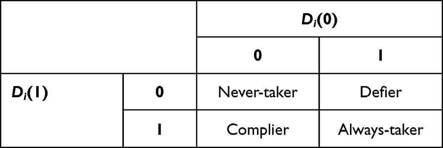Table 1 Subpopulations Classified by Di(1) and Di(0)

We adopt the assumptions for a confounded instrument, which were developed by Abadie.¹² To state the IV assumptions, we define the propensity score of instrument (PS-IV) as the conditional probability of being encouraged to receive the treatment of interest given X_i, ie, . Under the IV assumptions listed below (Assumptions 1–3), along with the independence and exclusion restriction of the instrument, we can identify the local average treatment effect (LATE) based on regression or weighting methods.^12,13

Assumption 1 (Positivity): is between 0 and 1 for all x.

Assumption 2 (Nonzero average causal effect of Z on D): for all x.

Assumption 3 (Monotonicity): D_i(1)≥D_i(0) for all .

Instrumental Variable and One-Sided Noncompliance

We can demonstrate that including the IV in the PST model always violates the positivity assumption when noncompliance occurs only in one direction. This is called one-sided noncompliance. Without loss of generality, we assume that noncompliance occurs only in the Z_i=1 group. In this setup, monotonicity trivially holds, and there are only never-takers and compliers. Because there are only never-takers in the Z_i=0 group, D_i always equals 0 in the Z_i=0 group, ie, . Therefore, under one-sided noncompliance, including the IV in the PST model as a covariate consistently violates the positivity assumption.

Excluding the IV from the PST model can avoid this positivity violation under one-sided noncompliance. The PST with only X (PST-X) can be expressed as

(1)

Under one-sided noncompliance, we have , and therefore (Equation 1) becomes

(2)

(Equation 2) implies that if both and are between 0 and 1, which holds under Assumptions 1–3, then the PST-X satisfies the positivity assumption. Under one-sided noncompliance, because there are only never-takers and compliers, we have , which is called the compliance score,¹⁴ which is between 0 and 1 by Lemma 2.1 of Abadie.¹²

The positivity violation resulting from including the IV with one-sided noncompliance makes bias and variance inflation occur due to the subjects whose true PSs are exactly zeros in the Z_i=0 group. The predicted values of these extreme PSs would be very close to 0s and lead to large inverse probability weights. The bias occurs when we target the ATE population, which includes units of the Z_i=0 group that receive the treatment, because those units cannot exist theoretically.¹¹ In other words, the data are not informative about the effect of treatment among patients who were never treated. The extreme PSs also inflate the variance of the IPTW estimator based on the asymptotic variances in (Equations 10 and 11).

Instrumental Variable and Two-Sided Noncompliance

In this section, we consider two-sided noncompliance, where noncompliance can occur in both Z_i=1 and Z_i=0 groups. Two-sided noncompliance does not necessarily constitute a violation of positivity, as opposed to one-sided noncompliance. However, even in cases of two-sided noncompliance, we can demonstrate that excluding the IV from the PST model can alleviate a potential violation of positivity.

Under two-sided noncompliance, monotonicity excludes defiers from the population. Hereafter we will refer to the PST conditional on both IV and X as PST-ZX. We can demonstrate the relationships between the PST-ZX and the compliance class probabilities below:

(3)

and

(4)

Based on (Equations 1, 3 and 4), under two-sided noncompliance, the PST-X can be written as

(5)

A critical difference between the PST-X and PST-ZX is that the PST-X is a smoothed version of the PST-ZX. This can be observed by noting that the PST-ZX in (Equations 3 and 4) can be written as one equation:

(6)

where I(z = 1) equals 1 if z = 1 and 0 otherwise. (Equation 6) is equivalent to (Equation 3) for z = 0 and (Equation 4) for z = 1. It is also equivalent to (Equation 5) if I(z = 1) is replaced by its expectation conditional on X. Because is a probability, it is less extreme than the indicator itself.

(Equations 5 and 6) imply that the PST-X is always between (Equations 3 and 4):

(7)

which implies that under the IV assumptions, the PST-X is less subject to a potential violation of positivity than the PST-ZX. There are two important special cases to demonstrate (Equation 7). If the relative population size of always-takers is minimal, ie, , then . Here, the situation is like one-sided noncompliance because subjects in the Z_i=0 group are very unlikely to receive active treatment, and the PST-ZX could be very close to 0. However, in the same situation, the PST-X is away from 0 by at least based on (Equation 5). As the opposite example, if the relative population size of never-takers is very small, ie, , then . In the same situation, however, the PST-X is away from 1 by at least .

Impacts of an IV Regressor on the IPTW Bias

Suppose that an IV has a strong monotonicity that induces one-sided noncompliance. In that case, the number of subjects who violate positivity is NPr(Z_i=0), when this IV is included in the PST model (PST-ZX). Therefore, the bias using PST-ZX is more affected by Pr(Z_i=1) rather than the IV strength; the bias will decrease as Pr(Z_i=1) increases, as demonstrated in our simulations. When this IV is excluded from the PST model (PST-X), the PST is expressed as the compliance score multiplied by the PS-IV, , and therefore PST-X is affected by both compliance score and PS-IV. Even though there is no complete positivity violation in this PST-X, finite sample bias could exist if either the compliance score or PS-IV is close to 0.

If an IV has a monotonicity that induces two-sided noncompliance, a positivity violation does not necessarily occur. However, there could be a near violation of positivity when using PST-ZX if the probabilities of an always-taker are minimal, say 0.05. In this case, although less severe than one-sided noncompliance, which brings the complete positivity violation, finite sample bias could exist.

Impacts of an IV Regressor on the IPTW Variance

Under strong ignorability of treatment, Wooldridge⁵ demonstrated that adjusting for IVs in ordinary least squares (OLS) inflates the asymptotic variance of the treatment effect estimate under a linear outcome model whenever the IVs are correlated with the treatment (equations 2.12, and 2.13 of Wooldridge⁵). To demonstrate this variance inflation by IVs, he adopted the assumptions of constant treatment effects, homoscedastic error variance, and exclusion restriction of the IVs. With these assumptions, the asymptotic variance of the treatment effect estimate without the IVs is the error variance divided by the variance of the treatment variable. However, when the IVs are adjusted in OLS, Wooldridge⁵ showed that the asymptotic variance is the error variance divided by the variance of the linear projection error from partialling the IVs out of the treatment. Therefore, if the IVs are more correlated with the treatment, the variance of the projection error will reduce while the error variance unchanged, and therefore the asymptotic variance will inflate. Wooldridge⁵ called this phenomenon multicollinearity.

We demonstrate that similar results to the OLS results can be obtained for the IPTW estimators. Based on Li et al¹⁰, the asymptotic variance of the IPTW estimator under constant treatment effects is

(8)

where for . Employing the homoskedasticity assumption like Wooldridge,⁵ we write . Then, (Equation 8) can be written as

(9)

(Equation 9) is the error variance V multiplied by the average of the inverse of the treatment variance conditional on the covariates, similar to the variance formula presented by Wooldridge.⁵

It is worthwhile to note that the homoskedasticity assumption and the exclusion restriction together imply that adjusting for the IV in the PST model does not affect the conditional variances of the potential outcomes, ie, for . Therefore, conditional on the IV, (Equation 9) becomes

(10)

(Equations 9 and 10) tend to be minimized when and are close to 0.5, respectively. Therefore, (Equation 10) demonstrates that monotonicity brings in multicollinearity because adjusting for the IV in the PST model can inflate the variance without reducing the error variance.

To understand the behavior of (Equation 10), we express it as the error variance V multiplied by the sum of the following weighted expectations:

(11)

and

(12)

Under one-sided noncompliance, , and therefore, the estimated value of (Equation 12) could be very large in the sample. However, (Equation 9) could be also very large because the PST-X is a product of two probabilities, , under one-sided noncompliance, which can make PST-X be very small when either the compliance score or PS-IV is close to 0. Therefore, if the IV prevalence is small or IV is weak, then the majority of PST-X would be distributed near 0, which would inflate the variance. Our simulations show that PST-X can suffer from a near positivity violation and give less precise IPTW estimates than PST-ZX.

Under two-sided noncompliance without a positivity violation, (Equation 10) is likely to be greater than (Equation 9), because in (Equation 9) is between and in (Equations 11 and 12), as implied by (Equations 5 and 7). Therefore, excluding the IV from the PST model will reduce the variance.

An interesting scenario of two-sided noncompliance is when the probabilities of an always-taker are almost zero, say 0.05, and thus there is a near violation of positivity. As in one-sided noncompliance, the IPTW estimates based on PST-X and PST-ZX may exhibit both finite sample bias and inflated variance. However, the relative efficiency of using PST-X rather than PST-ZX would be much better than the case of one-sided noncompliance because PST-X is expressed as the product of two probabilities plus a small number (probability of an always-taker), and therefore, much less likely to be almost 0. In fact, our simulations show that the relative efficiency of PST-X over PST-ZX is the greatest under the near positivity violation.

Simulation Study

Simulation Models

In this section, we conducted simulations to empirically demonstrate how including a binary IV in the PST model affects the distribution of the PS and the accuracy of the IPTW estimator. Adopting the simulation design of Choi et al,¹⁵ we generated six normal random variates, X₁–X₆, with mean zeros and paired correlation coefficients of 0.5. The PS-IV was a logistic function of these covariates:

We generated the instrument Z from a Bernoulli distribution with a success probability of . The following parameter values were used for the PS-IV model:

and the intercept β₀ was determined to implement three different degrees of IV prevalence, Pr(Z=1)=0.1, 0.3, and 0.5. For convenience, we referred to these scenarios as low, moderate, and high prevalence of the IV.

For one-sided noncompliance, we generated the latent compliance class U as a binary variable, with 1 and 0 indicating a complier and a never-taker, respectively. The probability of being a complier, ie, the compliance score, was generated from the following logistic model:

where . Because there are only compliers and never-takers under one-sided noncompliance, a never-taker’s probability was . We chose the intercept λ₀ to have four different degrees of overall IV strength: Pr(U)= 0.1, 0.3, 0.5, and 0.7. For convenience, we referred to the scenarios when Pr(U)= 0.1, 0.3, 0.5, and 0.7 as “Weak IV”, “Mild IV”, “Moderate IV”, and “Strong IV”, respectively. To simulate one-sided noncompliance, the treatment variable was D=ZU, which equaled Z for compliers and 0 for never-takers.

For two-sided noncompliance, we generated the latent compliance class U as a nominal category variable, with 0, 1, and 2 indicating a never-taker, an always-taker, and a complier, respectively. The same compliance model and values of λ₀ were used to generate the compliance probabilities and desired degrees of overall IV strength (0.1, 0.3, 0.5, and 0.7) as those used for one-sided noncompliance. However, we considered two types of two-sided noncompliance. One type had a near violation of positivity and the other did not have such a violation. Based on (Equations 3 and 4), the positivity violation occurs when the probabilities of an always-taker are exactly equal to zeros. Therefore, we generated data for the near positivity violation by letting the probabilities of an always-taker be very close to 0. More specifically, we let Pr(U=a)=0.05. For the other type of two-sided noncompliance, we allow the possibilities of being a never-taker and an always-taker be the same as . In this case, practically the PSs are unlikely to be 0s or 1s. The treatment variable was , which equaled Z for compliers, 0 for never-takers, and 1 for always-takers.

For outcome Y, we considered the following mean model:

where v₀=0 and . The outcome Y was generated from a normal distribution with mean and standard deviation of 1.5. Because the mean model implied a constant treatment effect, the LATE and ATE were equal to . In addition, we considered heterogeneous treatment effects by replacing with , where the treatment effects vary based on . However, the ATE was still equal to 1 because . The results for heterogeneous treatment effects were very similar to those of homogeneous treatment effects , thus reported in Supplementary Tables 1–3.

Simulation Results

We investigated the impact of including the IV in the PST model on the bias and variance of the IPTW estimator using the simulated datasets with a sample size of 3000. The values of the PST-X were estimated based on a generalized additive model (GAM) with a logit link and the smoothing splines (4 degrees of freedom) of the covariates. The values of the PST-ZX were estimated similarly, but the IV was added to the models. Based on the estimated values of PST-X and PST-ZX, we calculated the IPTW estimates and summarized the bias and empirical variances over the 500 simulated datasets. In addition, relative efficiency was calculated as the variance of the IPTW estimate using the PST-ZX divided by that based on the PST-X. A relative efficiency greater than 1 indicates that the IPTW estimate is more precise when the PST-X is used instead of the PST-ZX.

We compared the distributions of the PST-X and PST-ZX based on the histograms for the true values from the simulated data set with a sample size of 10,000 for each of the twelve scenarios. Figures 1–3 shows the PS distributions under one-sided noncompliance, two-sided noncompliance with a near positivity violation, and two-sided noncompliance without a positivity violation. It is worth noting that the IV groups have two modes of PST-ZX (Z = 0 on the left and Z = 1 on the right), and the distance between them represents the overall IV strength. As the IV is stronger, the ranges of both PST-X and PST-ZX become wider, but the range of the PST-ZX was wider than that of the PST-X. We use Figures 1–3 to interpret the simulation results.

Figure 1 Distributions of two versions of the propensity scores across the twelve simulation scenarios that differ by instrumental prevalence and strength under one-sided noncompliance with a complete violation of positivity. The red curves indicate the propensity scores when an instrumental variable (IV) is not adjusted for (PST-X). The bule curves indicate those when the IV is adjusted for (PST-ZX). Abbreviations: PS, propensity score; PST-X, propensity score of treatment conditional on pretreatment variables only; PST-ZX, propensity score of treatment conditional on instrumental and pretreatment variables. Notes: (A–D), (E–H), and (I–L) represent the PS distributions when the IV prevalence is weak, moderate, and high, respectively. The association between the IV and treatment is weak, mild, moderate, and strong from top to bottom: (A, E and I) for weak IV; (B, F and J) for mild IV; (C, G and K) for moderate IV; (D, H, and L) for strong IV.

Figure 2 Distributions of two versions of the propensity scores across the twelve simulation scenarios that differ by instrumental prevalence and strength under two-sided noncompliance with a near violation of positivity. The red curves indicate the propensity scores when an instrumental variable (IV) is not adjusted for (PST-X). The bule curves indicate those when the IV is adjusted for (PST-ZX). Abbreviations: PS, propensity score; PST-X, propensity score of treatment conditional on pretreatment variables only; PST-ZX, propensity score of treatment conditional on instrumental and pretreatment variables. Notes: (A–D), (E–H), and (I–L) represent the PS distributions when the IV prevalence is weak, moderate, and high, respectively. The association between the IV and treatment is weak, mild, moderate, and strong from top to bottom: (A, E and I) for weak IV; (B, F and J) for mild IV; (C, G and K) for moderate IV; (D, H and L) for strong IV.

Figure 3 Distributions of two versions of the propensity scores across the twelve simulation scenarios that differ by instrumental prevalence and strength under two-sided noncompliance with no violation of positivity. The red curves indicate the propensity scores when an instrumental variable (IV) is not adjusted for (PST-X). The bule curves indicate those when the IV is adjusted for (PST-ZX). Abbreviations: PS, propensity score; PST-X, propensity score of treatment conditional on pretreatment variables only; PST-ZX, propensity score of treatment conditional on instrumental and pretreatment variables. Notes: (A–D), (E–H), and (I–L) represent the PS distributions when the IV prevalence is weak, moderate, and high, respectively. The association between the IV and treatment is weak, mild, moderate, and strong from top to bottom: (A, E and I) for weak IV; (B, F, and J) for mild IV; (C, G and K) for moderate IV; (D, H and L) for strong IV.

Table 2 shows the absolute bias, empirical variances, multiplied by 1000, of the IPTW estimates based on the two types of PSs, PST-X and PST-ZX, and relative efficiency of PST-X over PST-ZX for the twelve simulation scenarios under one-sided noncompliance. Using PST-ZX induced significant bias in the IPTW estimates, ranging from 0.56 to 1.10, and the magnitude of the bias was dependent on the IV prevalence as it decreased as the IV prevalence increased. This result is consistent with our theoretical result that all PSs are exactly zeros for the Z = 0 group under one-sided noncompliance. Therefore, a greater IV prevalence implies fewer observations with a positivity violation, which reduces the amount of bias. Even though much less severe than the bias of PST-ZX, PST-X also yielded some finite sample bias, mainly because some PSs were very close to 0s when either IV prevalence or IV strength was close to 0. Based on Figure 1, the mode of the distribution of PST-X was approximately the IV prevalence times overall IV strength. Therefore, as shown by our simulations, the bias of PST-X decreased as the IV prevalence or IV strength increased. This observation was also consistent with our theoretical result that PST-X is represented by the PS-IV multiplied by the compliance score. The IPTW variances based on PST-X and PST-ZX decreased as the IV strengthened. Except one scenario (Pr(Z = 1)=0.5 and Pr(U = c)=0.7), PST-ZX gave smaller variances than PST-X, making the relative efficiency be less than 1. This result could be understood by investigating the PS distributions in Figure 1: even though the values of PST-ZX were exactly zeros for the Z = 0 group, which suffered from the positivity violation, those for the Z = 1 group had a better-behaved distribution, with a bell shape and the mode strictly away from 0, compared to the overall distribution of PST-X.

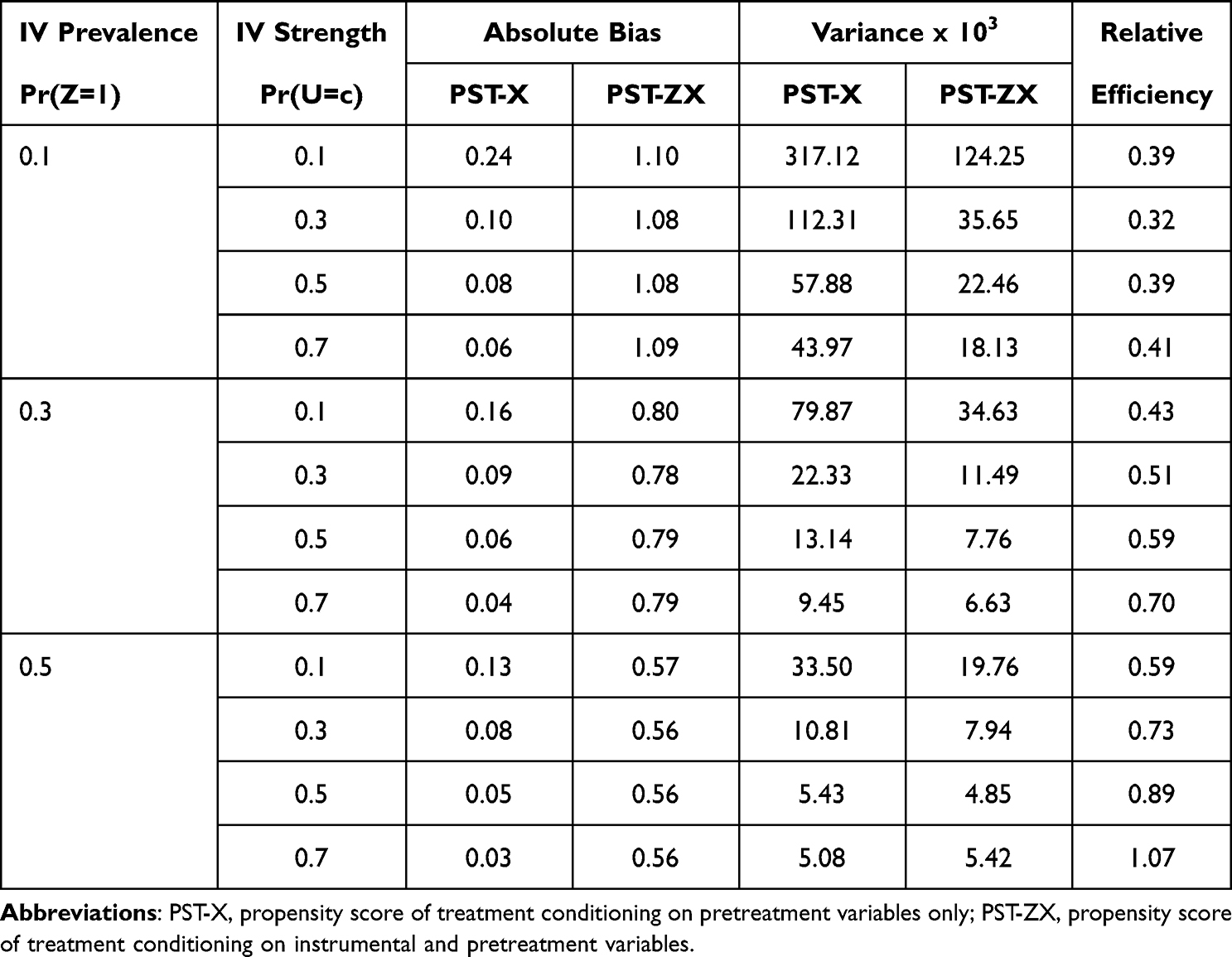Table 2 One-Sided Noncompliance with a Complete Violation of Positivity. Simulation Results for Comparing the Bias and Variances of Inverse-Probability-of-Treatment Weighted (IPTW) Estimators Based on Two Different Versions of the Propensity Scores

Table 3 shows the simulation results for two-sided noncompliance with a near positivity violation, where the probabilities of an always-taker were fixed at 0.05 rather than to 0, and therefore, the values of PST-X and PST-ZX were at least 0.05. Based on a comparison of Figures 1 and 2, setting the probabilities of an always-taker at 0.05 had the effect of moving the distributions of PST-X and PST-ZX uniformly to the right by approximately 0.05. The notable change in the transition from the complete positivity violation to the near violation was that the relative efficiency was greater than 1 for all twelve scenarios and increased as the IV prevalence or IV strength increased, with a maximized value of 4.29. This might be because the values of PST-X were always greater than 0.05, and therefore PST-X less suffered from positivity violations due to extreme PSs than in the cases of one-sided noncompliance. The bias also dramatically dropped by the transition from the complete violation to the near violation. PST-X was similarly or more biased than PST-ZX when Pr(Z=1)= 0.1 but less biased when Pr(Z=1) was 0.3 or 0.5.

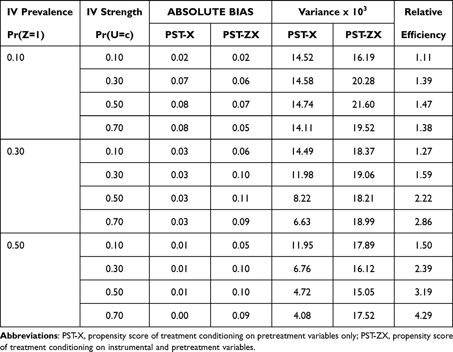Table 3 Two-Sided Noncompliance with a Near Violation of Positivity. Simulation Results for Comparing the Bias and Variances of Inverse-Probability-of-Treatment Weighted (IPTW) Estimators Based on Two Different Versions of the Propensity Scores

Table 4 shows the simulation results for two-sided noncompliance without a positivity violation. Figure 3 shows that both PST-X and PST-ZX had no significant densities around 0 or 1. Accordingly, the bias for both models was minimal, and therefore not reported. The relative efficiency was greater than 1 for all scenarios, with a maximized value of 1.98 at the largest IV prevalence and IV strength. In our simulations, , and therefore, the probabilities of an always-taker decrease as those of a complier increase, which happens in practice because the probability sum must not exceed one for each individual. Accordingly, Pr(U=a|X) is distributed around 0.45, 0.35, 0.25, and 0.15 when Pr(U=c)= 0.1, 0.3, 0.5, and 0.7, respectively. As a result, as the IV became stronger, the mode of PST-X moved to the left (Figure 3), and this made both IPTW variance and relative efficiency increase. This was consistent with our theoretical result that PST-X is less extreme than the two versions of PST-ZX (Z = 1 and Z = 0).

Table 4 Two-Sided Noncompliance Without a Positivity Violation. Simulation Results for Comparing the Variances of Inverse-Probability-of-Treatment Weighted (IPTW) Estimators Based on Two Different Versions of the Propensity Scores

Discussion

We have demonstrated that using an IV as a covariate for the PST can increase the bias and reduce the precision of an IPTW estimator. We have demonstrated this using the potential outcome framework of Angrist et al⁷ and the IV assumptions for the estimation of the LATE with covariates.¹² Particularly, we considered two different strengths of monotonicity that give both one-sided and two-sided noncompliance. An interesting theoretical finding was that the PST-X can be shown to be a smoothed version of the PST-ZX.

Our theoretical work and simulation studies demonstrated that adjusting for an IV with one-sided noncompliance yields a complete violation of positivity, resulting in substantial bias in the IPTW estimator. This bias can be reduced when the complete positivity violation is alleviated so that no subjects have PSs exactly equal to 0s. This near positivity violation can happen under two-sided noncompliance when the probabilities of an always-taker are minimal but not exactly 0s, and such an IV is adjusted for. However, the IV with the near positivity violation inflates the IPTW variance. Under two-sided noncompliance without a positivity violation, significant bias is not observed for both model approaches (PST-X and PST-ZX) but adjusting for the IV still inflates the IPTW variance.

Strong ignorability is a fundamental assumption for PS weighted analysis. If X is a set of the covariates that satisfies strong ignorability, then our study results imply that an IV must be excluded from the PST model. However, strong ignorability is not empirically verifiable so a researcher can never know that it is satisfied without sufficient subject matter knowledge. If we can assume that one-sided noncompliance holds and the IV is valid, we can test strong ignorability using the equality between the LATE for the treated (LATT) and the average treatment effect for the treated (ATT). Accordingly, Donald et al¹⁶ developed a Durbin-Wu-Hausman test of whether D is unconfounded conditional on X by testing the equality between LATT and ATT. If this equality is not rejected, then the unconfoundedness of D is supported, which implies that the IPTW estimator is a consistent estimator for ATE. In this case, the IV should not be included in the PST to avoid positivity violations.

We investigated how including the IV with monotonicity impacts the positivity of the PS. Among the authors who studied IVs as bias amplifiers, Ding et al⁶ considered general settings where there is unmeasured confounding between the treatment and outcome. With unmeasured confounding, the IPTW estimator based on the PST-X is biased for the ATE, and therefore, our approach, which relies on only the monotonicity between Z and D, is not sufficient to determine whether using an IV as a covariate for the PST is beneficial or harmful. Ding et al⁶ employed a set of monotonicity assumptions for three pairs of the associations between the outcome, treatment, and unmeasured confounder and theoretically demonstrated that adjusting for an IV amplifies the bias of the unadjusted estimator.

A perfect IV is strongly related to the treatment but not to the outcome directly. An interesting case arises when there are variables, so-called imperfect IVs strongly related to treatment but only weakly related to the outcome. Pearl¹⁷ demonstrated that an imperfect IV can hardly become a bias reducer under a linear structural model with an unmeasured confounder. Using directed acyclic graphs, Brookhart et al¹⁸ discussed how, in the presence of unmeasured confounding, an IV could amplify bias and behave like a confounder, a phenomenon they termed Z-bias. Myers et al¹⁹ reported evidence of bias amplification in an extensive simulation study. Brookhart et al⁴ conducted simulation experiments as changing the strength of association between a single confounder and both the outcome and treatment and showed that including an imperfect IV can be detrimental to an effect estimate in a mean squared error sense. Even though our study assumes a valid IV, our findings should also apply to an imperfect IV, because a positivity violation caused by one-sided noncompliance and variance inflation due to extreme PSs under two-sided noncompliance are obtained based on only the relationship between the IV and treatment.

The practical implications of our results largely depend on the context. If the set of candidate covariates does not contain variables that could plausibly be IVs, there is probably little risk for creating a rich model using all baseline covariates. If there are variables that are thought to be IVs, these should be considered for exclusion from the PST. But if there exist variables that are strongly related to treatment, but the researcher is uncertain whether they have an independent relationship with the outcome, it would be reasonable to do multiple analysis that include and exclude these potential IVs. In addition, if the number of covariates is large, as in a study of right heart catheterization,²⁰ we would want to investigate whether any covariates increase the variability of the PSs. In this case, variable selection methods for causal inference, such as outcome-adaptive lasso,²¹ could be helpful to exclude IVs from the PST model.

Conclusion

This paper shows that including an IV with monotonicity in the PST model can cause a complete or near violation of positivity. The key result was that the PS, without adjusting for the IV, is a smoothed version of the PS using the IV. Our theoretical and numerical investigations demonstrated that excluding the IV from the PST model can reduce the bias in the presence of one-sided noncompliance and improve the precision in the presence of two-sided noncompliance.

References

1. VanderWeele TJ. Principles of confounder selection. Eur J Epidemiol. 2019;34(3):211–219. doi:10.1007/s10654-019-00494-6
2. Rosenbaum PR, Rubin DB. The central role of the propensity score in observational studies for causal effects. Biometrika. 1983;70(1):41–55. doi:10.1093/biomet/70.1.41
3. Hirano K, Imbens GW. Estimation of causal effects using propensity score weighting: an application to data on right heart catheterization. Health Serv Outcomes Res Methodol. 2001;2(3/4):259–278. doi:10.1023/A:1020371312283
4. Brookhart MA, Schneeweiss S, Rothman KJ, Glynn RJ, Avorn J, Stürmer T. Variable selection for propensity score models. Am J Epidemiol. 2006;163(12):1149–1156. doi:10.1093/aje/kwj149
5. Wooldridge JM. Should instrumental variables be used as matching variables? Res Econ. 2016;70(2):232–237. doi:10.1016/j.rie.2016.01.001
6. Ding P, Vanderweele TJ, Robins JM. Instrumental variables as bias amplifiers with general outcome and confounding. Biometrika. 2017;104(2):291–302. doi:10.1093/biomet/asx009
7. Angrist JD, Imbens GW, Rubin DB. Identification of causal effects using instrumental variables. J Am Stat Assoc. 1996;91(434):444–455. doi:10.1080/01621459.1996.10476902
8. Imbens GW, Rubin DB. Causal Inference for Statistics, Social, and Biomedical Sciences: An Introduction.
9. Lunceford JK, Davidian M. Stratification and weighting via the propensity score in estimation of causal treatment effects: a comparative study. Statist Med. 2004;23(19):2937–2960. doi:10.1002/sim.1903
10. Li F, Morgan KL, Zaslavsky AM. Balancing covariates via propensity score weighting. J Am Stat Assoc. 2018;113(521):390–400. doi:10.1080/01621459.2016.1260466
11. Petersen ML, Porter KE, Gruber S, Wang Y, Van Der Laan MJ. Diagnosing and responding to violations in the positivity assumption. Stat Methods Med Res. 2012;21(1):31–54. doi:10.1177/0962280210386207
12. Abadie A. Semiparametric instrumental variable estimation of treatment response models. J Econom. 2003;113(2):231–263. doi:10.1016/S0304-4076(02)00201-4
13. Tan Z. Regression and weighting methods for causal inference using instrumental variables. J Am Stat Assoc. 2006;101(476):1607–1618. doi:10.1198/016214505000001366
14. Aronow PM, Carnegie A. Beyond LATE: estimation of the average treatment effect with an instrumental variable. Polit Anal. 2013;21(4):492–506. doi:10.1093/pan/mpt013
15. Choi BY. Instrumental variable estimation of weighted local average treatment effects. Stat Papers. 2023. doi:10.1007/s00362-023-01415-2
16. Donald SG, Hsu YC, Lieli RP. Testing the unconfoundedness assumption via inverse probability weighted estimators of (L)ATT. J Bus Econ Stat. 2014;32(3):395–415. doi:10.1080/07350015.2014.888290
17. Pearl J. On a class of bias-amplifying variables that endanger effect estimates. arXiv preprint arXiv. 2012;2012:1. doi:10.48550/ARXIV.1203.3503
18. Brookhart MA, Stürmer T, Glynn RJ, Rassen J, Schneeweiss S. Confounding control in healthcare database research: challenges and potential approaches. Med Care. 2010;48(6):S114–S120. doi:10.1097/MLR.0b013e3181dbebe3
19. Myers JA, Rassen JA, Gagne JJ, et al. Effects of adjusting for instrumental variables on bias and precision of effect estimates. Am J Epidemiol. 2011;174(11):1213–1222. doi:10.1093/aje/kwr364
20. Connors AF. The effectiveness of right heart catheterization in the initial care of critically ill patients. SUPPORT Investigators. J AM Med Assoc. 1996;276(11):889–897. doi:10.1001/jama.276.11.889
21. Shortreed SM, Ertefaie A. Outcome‐adaptive lasso: variable selection for causal inference. Biometrics. 2017;73(4):1111–1122. doi:10.1111/biom.12679
© 2023 The Author(s). This work is published and licensed by Dove Medical Press Limited. The
full terms of this license are available at https://www.dovepress.com/terms
and incorporate the Creative Commons Attribution
- Non Commercial (unported, 3.0) License.
By accessing the work you hereby accept the Terms. Non-commercial uses of the work are permitted
without any further permission from Dove Medical Press Limited, provided the work is properly
attributed. For permission for commercial use of this work, please see paragraphs 4.2 and 5 of our Terms.