Making Statistics Clinically Meaningful

Introduction

Clinical epidemiology is a basic science that supports clinicians in making informed prevention, diagnostic and treatment decisions.¹ A core principle of clinical epidemiology is the use of robust statistical methods alongside transparent interpretation and communication of statistical results. These results need to be useful and relevant, not only for clinicians making diagnostic and treatment decisions but also for population health researchers informing public health policy and disease prevention strategies. Many studies are statistically sound but are still difficult to translate into clinical decision-making because the results are not presented in a clinically interpretable way.

In this article we provide an informed perspective with illustrative examples rather than a comprehensive review, to discuss how applying statistical thinking at each stage of the research process can enhance the clinical meaningfulness of statistical findings. We use examples from different study designs to illustrate these issues considering approaches to presenting results and providing examples using i) simulation and ii) published data from observational studies based on primary data collection and registry data, as well as randomized clinical trials (RCTs). Through these examples, we illustrate strategies for maximizing the usefulness and impact of statistical results. The principles illustrated in this article are relevant to most quantitative research studies and complement work in the translational statistics space.² Our aim is to stimulate dialogue among clinicians, epidemiologists, statisticians and data scientists about how statistics, in the broadest sense, can be made more clinically relevant. An online document provides additional reading for the unreferenced statistical terms used in this article (supplement 1).

What Do We Mean by Clinically Meaningful?

Evidence-based medicine is the present-day term for the application of scientific evidence including principles of clinical epidemiology to the care of patients.^1,3 Due to the growth of evidence-based medicine, evidence is readily available, often in large quantities that are difficult to synthesize and interpret. This challenge becomes particularly evident when clinicians seek to translate research findings into clinical decision-making in the era of personalized medicine. For example, once a diagnosis has been established, the clinician and patient must collaborate to determine the most appropriate care plan for that individual patient, weighing expected benefits against potential side effects. Doing so requires evidence that is interpretable, relevant and applicable to the clinical context. However, interpretation is complicated by the varied nature of clinical outcomes, which range from “hard” objective endpoints or outcomes such as mortality, to “soft” subjective endpoints such as symptom relief.⁴

It is important that results are accessible to clinicians who often work in fast-paced environments and, particularly for generalists, may treat patients with wide-ranging symptoms and diagnoses. Key findings therefore need to be presented clearly. When clinicians are unfamiliar with specific statistical concepts, there is a shared responsibility to foster learning and clarify what information is needed to enable results to be translated into the clinical framework.

While it is arguably the responsibility of statisticians/data scientists to present results in a way that aligns with clinical needs, and the responsibility of clinicians to understand the underlying medical concepts, it is essential to that the questions asked and the results produced are relevant to the clinical need and therefore clinically meaningful. For these reasons it is essential that clinicians, epidemiologists and statisticians/data scientists work together throughout the planning, information-gathering, processing and dissemination stages to maximize the usefulness of the information produced.

Clinical Meaningfulness: The Research Process

In this section, we take a whistlestop tour through the traditional research process from formulating a research question, to selecting an appropriate study design, to conducting statistical analyses. We seek to highlight key principles that help ensure the statistics are clinically meaningful (Figure 1). We do not focus primarily on hypothesis-generating studies, although we return to them later in the article. From herein we refer to “statisticians and data scientists” as “statisticians” for conciseness.

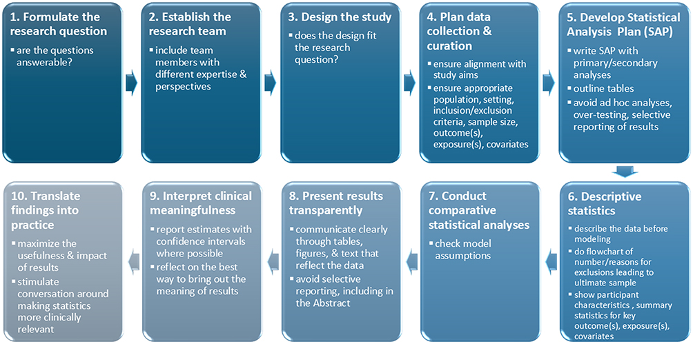Figure 1 Summary of the research process.

At the design and planning stage, it is important to review the study aims and research questions to ensure that they are clearly defined and answerable. The next step is to determine whether the proposed study design addresses these questions and whether it is practical and feasible to implement. Following this, a data collection protocol must be developed if primary data are required, or a data curation protocol if existing data, such as a registry or administrative dataset, will be used. Data collection must align closely with the study aims and include appropriate outcome(s), exposures, covariates, population, setting, inclusion/exclusion criteria, and sample size considerations. Whether planning new data collection or assessing the feasibility of using existing data, there is a balance between obtaining sufficient data to address the research questions and collecting additional data that may be useful later. Expanding the data collection may, however, decrease data quality and increase missingness, eg. through participant fatigue, non-response, or added time and resource demands. If introducing new data collection tools or procedures, piloting them is advisable. Finally, data checking is vital, preferably during the study period, so that any issues can be identified and protocols adjusted while changes are still possible.

Before analyzing the data, it is good practice to write a statistical analysis plan (SAP) that specifies the primary and secondary analyses and includes outline tables. This helps prevent ad hoc analyses, excessive testing or data-dredging, and selective reporting of results. These SAPs are sometimes published with the study protocol⁵ or registered online⁶ before analysis to ensure transparent pre-planned methods. The SAP is developed collaboratively by the project team members, including clinicians, epidemiologists and statisticians, and is a useful bridge between clinical insight and methodological thinking. Revisions to a SAP may be needed for several reasons including: i) if preliminary descriptive analyses reveal very small cell sizes that could compromise confidentiality and legislation, ii) if unexpected missing data are identified in routine or registry sources, iii) if recruitment and/or outcome rates are different from those expected in the study population or iv) if new information comes to light that affects the design or analysis. Whenever the SAP is changed, it is important to document a clear chronology of changes. This may involve a formal amendment if the original protocol or SAP have been published⁷ to ensure ongoing transparency.

It is important to describe the data before doing any modeling. This includes presenting a flowchart showing who was excluded and ultimately included, summarizing participant characteristics and reporting key outcomes, exposures, and covariates. Such information enables clinicians to understand who participated in the study and helps them assess how applicable the findings may be to their own patient populations. When conducting analyses, it is important to examine the comparability of people with missing or excluded data relative to those included, and to verify that model assumptions are met. When appropriate, and particularly in large datasets, stratified descriptive analyses can be valuable before undertaking multivariable modeling. These analyses can reveal patterns of effect modification and confounding that may be obscured in regression models. This approach strengthens the validity and interpretability of subsequent regression models and enables researchers to engage more deeply with the underlying data structure.

When reporting results, we address the study aims by communicating clearly through tables, figures, text, that are true reflections of the data.⁸ Abstracts, in particular, are prone to selective reporting.⁹ If possible, results should be presented as estimates with measures of precision such as confidence or credible intervals, and p-values when they aid interpretation. Care is needed to avoid drawing inappropriate causal conclusions from observational data. All these aspects of design are crucial to producing work that is clinically interpretable Nonetheless, we often spend limited time considering how best to convey the meaning of results and what they mean in practice. These issues will be the focus of the remainder of this article.

Clinical Meaningfulness: Interpreting Results – P-Values and Estimates

P-Values

It has long been considered good practice to report estimates with confidence intervals (or credible intervals) where possible, rather than relying on p-values as a measure of the size of difference or strength of association.¹⁰ The p-value is a measure of the weight of evidence for or against a null hypothesis being tested but is often presented and interpreted as a dichotomous entity, “significant” versus “non-significant”, using an arbitrary cut-off, eg p<0.05, to define what is meant by “significant”. This practice is tantalizingly attractive in facilitating fast decision-making but is deeply flawed since a p-value provides no information about the strength of effect and so is of limited use in summarizing and interpreting a study’s findings. Another problem with the sole use of p-values to evaluate study results is that the p-value is influenced by the sample size, n, as well as the actual effect size. Thus, the same effect size can yield very different p-values depending on the value of n. For example: if Pearson’s correlation coefficient = +0.3, n=30 then p=0.11, whereas the same correlation, +0.3 with n=200 has p<0.001 (Figure 2Aand Figure 2B). This property of p-values, that they are related to the study size as well as the estimate, means that “not significant” cannot be interpreted as implying that there is “no difference” or “no association”, as is commonly and incorrectly done. Further, the dichotomization of results as significant/non-significant that imply important/non-important is a factor contributing to the observed excess of statistically significant findings in the published literature, ie publication bias.

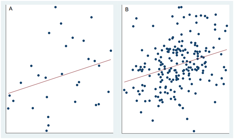Figure 2 (A and B) Two datasets1, same correlation, different sample size, different p-value. Datasets were simulated to have Pearson’s correlation = +0.3. (A) r = +0.3, n=20, p=0.11. (B) r = +0.3, n=200, p<0.001.

P-values therefore incorporate information about the size of effect and the sample size but they do not in themselves adjust for confounding and/or systematic biases which are common in non-randomized designs - an “adjusted p-value” usually has a different meaning to an “adjusted estimate”. P -values can therefore give a false sense of certainty even when substantial bias may be present.

For all of these reasons, p-values cannot be interpreted as a measure of the size or clinical relevance of a study’s effect, and their use as such is highly misleading. P-values cannot be used as a measure of clinical meaningfulness.^10–14

Estimates

However, the interpretation of estimates of effect size can also be challenging – how large must an effect be to be interpretable as “large”? Cohen has provided one way to handle this by proposing a standardized effect size measure, d=mean/standard deviation, with descriptors such that an effect size of 0.8 is considered “large”, 0.5 is “medium” and 0.2 is “small”, assuming the data follow a normal distribution.¹⁵ Cohen’s d is commonly applied and has clear merit when little information is available. However, it can be problematic when comparing populations, since a small effect may have substantially greater clinical impact in a sick or vulnerable population than in a healthy one.¹⁶ This can be illustrated using the example of birthweight. A mean difference of 180 g between infants born to non-smoking versus smoking women may have limited clinical implications among full-term infants, but the same difference may be far more consequential among preterm infants, who are already smaller and more vulnerable.

This issue has implications for the use of Minimal Clinically Important Difference (MCID), in sample size calculations. The MCID represents the smallest effect size that corresponds to a clinically meaningful change in the selected patient outcome. However, the same MCID may not be appropriate across different populations. For example, in systems with optimized discharge processes where prolonged length of stay is not necessary, even a modest reduction in hospital length of stay can have substantial system-level benefits. In a busy general hospital, freeing beds more quickly improves patient flow from the emergency department and enhances care for future patients through a more efficient use of resources, without detriment to current patients.¹⁷

Interpreting Differences Between Groups in Mean Outcome for Continuous Data

When a study outcome is continuous, we often summarize the data using measures of centrality and spread such as mean, median, standard deviation, inter-quartile range. However, comparing two or more groups, and interpretating between-group differences in mean values can be challenging from a clinical perspective. Common strategies to aid interpretation include observing the direction of effect, ranking of the sizes of differences across several groups, comparing observed differences with those previously reported by others, and using the p-value to define whether a difference is meaningful. These approaches, particularly the reliance on p-values,¹¹ are, as mentioned, of limited value in providing clinical meaning. For these reasons researchers sometimes dichotomize continuous outcomes to improve interpretability. Ideally, dichotomization employs a clinically relevant cut-point to identify persons at high risk. The proportions of high-risk participants can then be compared directly as risk differences, or as risk ratios. Some cut-points derive from established diagnostic thresholds, such as using sustained systolic blood pressure ≥130 mmHg or diastolic blood pressure ≥80 mmHg to classify hypertension. These thresholds may, however, be somewhat arbitrary. For example, during the COVID-19 pandemic, temperature criteria differed slightly between the UK and the US due to their reliance on Celsius vs Fahrenheit scales and rounding practices.

A problem may arise when an analysis based on a dichotomized outcome replaces one based on the original continuous measure. Dichotomization discards information, obscures underlying relations and reduces statistical power. For these reasons statisticians strongly advise against it.^18,19 A more robust strategy is to present the dichotomized analysis as a complementary secondary analysis alongside the primary analysis of the continuous outcome. Further examples are provided in more detail below.

Interpreting Differences in Mean Lung Function z-Scores

Z-scores are commonly used to standardize measurements, such as lung function, for age/sex/height. This allows a person’s lung function measurement to be interpreted relative to the value expected in a healthy individual of the same age/sex/height. To illustrate the challenges of interpreting mean z-scores and suggest a way forward, we use data from a cohort study that examined differences in a portfolio of lung function measures in teenage boys and girls born extremely preterm.²⁰ The lung function measures were analyzed as z-scores and showed better mean z-scores in girls than boys for 11 of the 16 measures, although only four of these differences were statistically significant. In order to help interpret the differences in mean z-scores, the difference in percentage below the lower limit of normal (LLN; below 5^th percentile) was calculated for all measures. For illustration, we only present results on FEV₁ (Table 1).

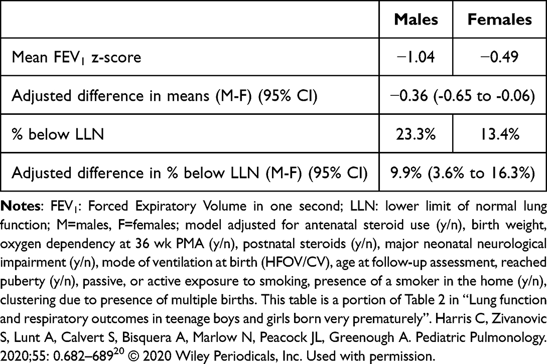Table 1 Presenting FEV1 z-Score Analyses as Means and % Below Lower Limit of Normal (LLN)20

By presenting the outcome both as mean z-scores and as the percentage of individuals below the LLN, we can see that an adjusted mean difference of 0.36 z-score units corresponds to 23.3% of boys versus 13.4% of girls falling below the LLN. This difference in percentages was easier to interpret and considered to be clinically important.

We note that in this example, a distributional approach was used to calculate the percentages below LLN rather than dichotomizing the raw data. The distributional approach has the advantage of preserving the precision and power of the estimated difference in percentages by using a function of the normal distribution in a similar way to the calculation of quantiles.^21,22

Interpreting the Meaning of Regression Coefficients

How we present regression coefficients affects the ease with which we can infer their clinical meaning. Simple steps include ensuring units are specified and that the direction of any differences is stated (as in Table 1) and described in chapter 10 of Peacock, Kerry and Balise.⁸ Beyond that, it is helpful to consider the range of both exposures and outcomes to see whether the coefficient would benefit from being scaled. Rather than reporting the effect per one-unit change in exposure—the default produced by regression models—researchers can present coefficients in terms of a “scaled” change that reflects a meaningful or realistic difference in exposure. This can highlight the practical impact of the exposure and facilitate comparison with other studies. The example below illustrates how scaling can help.

Scaling Estimates to Improve Interpretation

An analysis of data from the New Hampshire Birth Cohort Study compared how well two tobacco biomarkers, urinary cotinine and 4-(methylnitrosamino)-1-(3-pyridyl)-1-butanol (NNAL) in pregnant women, predicted outcomes of pregnancy.²³ Cotinine and NNAL were positively skewed and were analyzed on the log_e scale. The resulting coefficients were scaled to a one standard deviation increase in each of log cotinine and log NNAL to aid interpretation. Five continuous birth outcomes were analyzed: birthweight (g and z-score), gestational age (weeks), crown-heel length, and head circumference (z-score). The scaling allowed direct comparison of the predicted value of the two biomarkers, i.e. a comparison across the rows of Table 2. The paper also included two binary outcomes, small-for-gestational age, and preterm birth. The odds ratios for those were also similarly scaled.

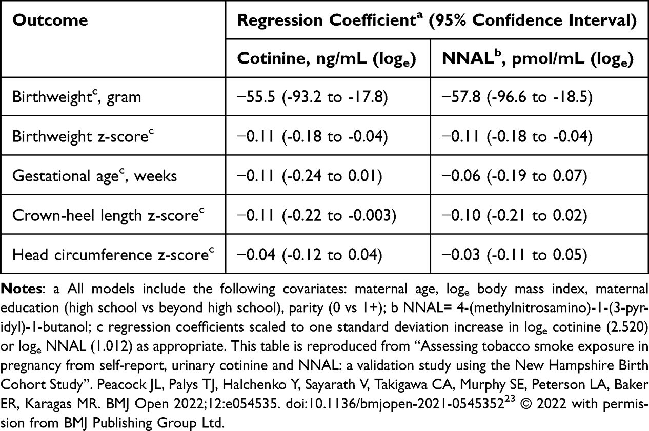Table 2 Regression Coefficients Scaled to One Standard Deviation Change in Exposure23

Using log₂

We note that sometimes researchers use logs to base 2, instead of base e, as we have here, for transforming skew exposure data. The mathematical effect of the transformation is unchanged but there is a useful interpretation of the regression coefficient on the log₂ scale as the change in outcome associated with a doubling of the exposure. For example, Signes-Pastor 2022²⁴ used a log₂ transformation of total urinary arsenic and reported that a doubling of total arsenic was associated with decreases in childhood cognitive abilities.

Interpreting Results Analyzed with the Outcome Analyzed on Logarithmic Scale

Logarithmic transformation is often applied to positively skewed outcomes such as serum creatinine to fulfill the requirement of a normal distribution when using a t test or normally distributed residuals when fitting a regression model. It is best practice to back-transform the data after analysis to get back to the natural scale and provide summary data that are more easily interpreted. In the case of a t test, the difference of means when back-transformed is the ratio of the geometric means, for example, comparing baseline serum creatinine in patients with peripheral vascular disease in survivors and those who died:

“Geometric means were: patients who survived, 97 compared to those who died, 108. The ratio of geometric means was 0.90, 95% CI: 0.79 to 1.02”.⁸

Note that the null hypothesis value is now 1, so the results indicate that mean serum creatinine values were 10% lower among survivors. The 95% CI indicates that the true population value might be as great as 21% lower or as high as 2% higher. See Peacock, Balise and Kerry, chapter 8 for more details.⁸

Interpreting Unadjusted and Adjusted Estimates

When a regression analysis includes covariates, it is often useful to report both the unadjusted estimates and covariate-adjusted estimates. We show below an extract from a table of the unadjusted and adjusted relative risks of any upper and any lower respiratory tract infection before and during the COVID-19 pandemic using data from the New Hampshire Birth Cohort Study.²⁵ Adjustment for several key covariates reduced the relative risk though not by much, strongly suggesting a real and sizable impact of stay-at-home orders in the State (Table 3).

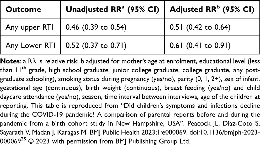Table 3 Caregiver Reported Upper and Lower Respiratory Tract Infections (RTI) Requiring a Doctor Visit in Children Age 0–11 Years Before and During the COVID-19 Pandemic25

Figure 3 provides another example, using data from the Danish National Patient Registry covering all Danish hospitals to investigate risk factors for VTE following a cancer diagnosis in a competing risks analysis.²⁶ This figure takes the tabulated data from the paper and displays them in a forest plot, making it easy to compare the unadjusted and adjusted subdistribution hazard ratios. The graphical presentation shows that after adjustment, most estimates move towards the null and become more precise (with narrower CIs). This simple presentation helps interpretation by clearly illustrating the impact of confounding on the estimates and thereby allowing the reader to judge whether the association is real.

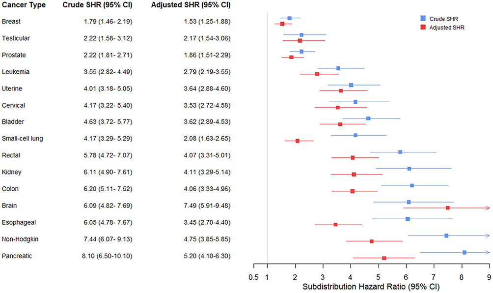Figure 3 Unadjusted and adjusted subdistribution hazard ratios for risk factors for venous thromboembolism (VTE) following cancer diagnosis in a competing risks analysis.26 The following covariates were adjusted for: age, sex, prior VTE (y/n), cancer stage (0-IV solid cancers), cancer type (categorized for VTE risk according to Khorana score classification).

There are many other examples of the challenges in uncovering the clinical meaning of regression analyses such as the modeling and interpretation of trends in regression models²⁷ among others.

Using and Interpreting Minimal Clinically Important Differences

In this final section we re-visit MCIDs which we introduced earlier. MCID is commonly used in study design to inform sample size calculations so that the target sample size is sufficient to be able to detect a clinically relevant change in a chosen patient outcome. This is important so that the findings from a study are most likely to inform clinicians and impact clinical decision making and patient outcomes. MCIDs are used in a range of study designs, including equivalence trials, which aim to demonstrate that two interventions produce clinically similar effects within a predefined margin of equivalence, and in non-inferiority trials that aim to demonstrate that a new intervention is not worse than a current intervention by more than a prespecified non-inferiority margin. MCIDs are also used as a benchmark against which an observed effect can be compared in order to determine whether or not it is clinically relevant.

Illustrating Clinical Impact in Vulnerable versus Healthy Populations

While MCIDs are useful for interpreting the clinical relevance of statistical results, challenges arise when applying an MCID derived from one population to another with different characteristics. In particular, it has been shown that a fixed exposure effect will have a greater clinical impact in vulnerable populations than in healthier ones.^16,28 This has implications for interpreting study findings in sub-populations defined by sociodemographic factors, as illustrated using data from over 28,000 mother/child pairs from the US Environmental influences on Child Health Outcomes (ECHO) study.²⁸

A simulation study using ECHO data examined the impact of an exposure that reduced mean birthweight by the same amount across sub-populations defined by sociodemographic categories. Below, we show the results for a 50g reduction in mean birthweight stratified by race. When the effect size is expressed as the change in mean birthweight, the effect is identical across groups (by design). However, when the effect is translated into its impact on the percentage of infants with low birthweight (LBW), the effect size becomes larger in the more vulnerable groups—those with lower mean birthweight. Figure 4 illustrates this, using data from this study showing that the effect size as LBW % points varies directly by race. For example among White participants, where the mean birthweight is approximately 3373g, the effect on LBW is around one percentage point. In contrast, among Black participants, whose mean birthweight is considerably lower at 3131g, the effect on LBW doubles to around two percentage points.

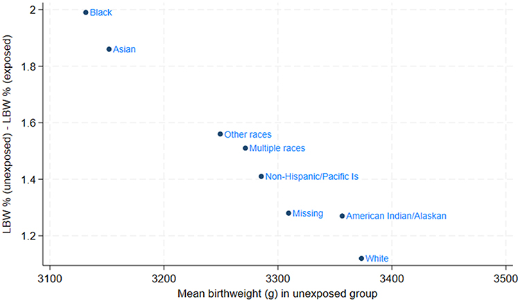Figure 4 Effect an exposure reducing mean birthweight by 50 g on LBW stratified by Race.28

Risks

Relative vs. Absolute Risks

Absolute risk varies with the underlying prevalence of disease in the study population. An intervention that reduces risk by 50%, ie RR=0.5, will look very different in absolute terms if baseline risk is 2% versus 20%, ie 2% → 1%, 20%→10%. If these differences are not taken into account, comparisons of clinical relevance across populations can be misleading. A well-known example is the association between CT-scan radiation exposure and subsequent cancer risk. Even if the increase in risk for an individual child undergoing a single CT scan is small, widespread use of CT scans in children with head injuries could lead to a meaningful increase in cancer incidence at the population level. For these reasons, it is important to report both relative and absolute risks to maximize the information available to make clinical decisions at both the individual patient and population level.

Odds ratios (ORs) are often used as proxies for relative risks (RRs), but caution is needed since unless the event in question has very low prevalence (rare disease assumption), the RR and OR calculated from the same set of data have different values, with the OR taking values farther from the null.

NNT/NNH

Number Needed to Treat (NNT) and Number Needed to Harm (NNH) are complementary measures that quantify the clinical impact of an intervention. NNT represents the average number of patients who must receive the intervention to prevent one additional adverse outcome compared with a control group. NNH reflects the number of patients who need to be treated for one additional harmful event to occur. Both measures are derived from absolute risk differences and provide an intuitive way to balance benefits and risks in clinical decision-making. A low NNT suggests high treatment efficacy, whereas a low NNH signals a higher likelihood of harm. Interpreting these measures together is essential for evaluating the net clinical benefit of a therapy. The risk–benefit ratio, often expressed as NNH divided by NNT, provides a single metric summarizing whether the expected benefit outweighs the potential harm; values greater than 1 indicate a favorable balance toward benefit. An example is given below from a RCT of the effect of treatment of gestational diabetes mellitus on pregnancy outcomes.²⁹ The main outcome was any serious perinatal complications (any vs none: death, shoulder dystocia, bone fracture, nerve palsy). NNT and NNH (Table 4) have been calculated from the results given in the paper.

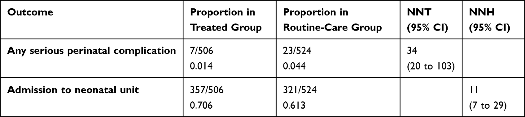Table 4 NNT and NNH from RCT of Treatment for Gestational Diabetes Mellitus on Pregnancy Outcomes29

Other Issues and Considerations

Here, we comment briefly on the challenges involved in deriving clinical meaning from high-dimensional ‘omics studies. These studies may be hypothesis-generating rather than hypothesis-testing which brings challenges for interpretation and reproducibility in the presence of multiple testing. Commonly approaches to adjust for multiple testing include Bonferroni, False Discovery Rate, and methodological work on adapting these approaches to complex ‘omics datasets is an active area of research (see Ebrahimpoor³⁰). A detailed review is beyond the scope of this article. The interpretation of small effects has been discussed earlier and is raised by Breton et al in relation to epigenetic studies in children’s environmental health where small observed effects may be considered meaningful when supported by consistency across studies.³¹

There are many other topics that could be included in a comprehensive review of clinical meaningfulness including the Bayesian decision framework for communicating clinical evidence and causal inference but these are beyond the scope of this article.

Finally, ensuring clinical meaningfulness is just the first step in translating robust evidence into change in practice.³²

Conclusions

In this paper, we have described and illustrated ways in which clinical meaning can be affected. First, it is challenging to infer robust clinical meaning where there are deficiencies in study design, data collection/measurement, or data analyses. However, even if these aspects are all adequately handled, sound clinical meaning can be obscured by avoidable issues in how results are presented for example inadequately annotated tables and figures, or poor formatting. As we have shown here, presenting the same information in complementary but different ways can often enhance clinical meaningfulness and support clearer interpretation.

Improving clinical meaningfulness takes time, for example to discuss, review, and revise results, and sometimes this step is overlooked because of time-pressures. We recommend that study teams prioritize interdisciplinary discussions of clinical meaningfulness from the outset and throughout the research process to ensure that the clinical impact of our work is maximized.