Evolution of Romania’s Economic Structure and Environment Degradation – An Assessment Through LMDI Decomposition Approach

Introduction

In the last decades, the contemporary societies and economies faced a significant transformation of the environmental paradigm. The current societies underwent global-scale transformations as an effect of an accelerated economic growth that at times turned aggressively against the environment, deteriorating the air we breathe. Air pollution is now the main feature of the industrial society that we are part of. As time passed and the new industrial facilities picked up, polluting agents started accumulating, particularly in the large urban conglomerates. The massive environmental pollution, the accentuated deforestation, the lack of green areas in the urban environment, the extension of the urban traffic and the lack of an integrated environmental policy or the faulty application of the existing environmental measures further accentuated the degradation of the population’s health.

The air quality has become one of the basically element in defining and improving the citizens’ state of health, as is well known that air pollution generates some of the most nefarious and hard-to-control effects on human health and the environment. The most environmental problems in South Eastern European countries, including Romania, have their origin in the rapid economic growth tendency, reorientation of traditional industrial production structures, often without respecting environmental requirements, unsustainable energy consumption, adding the growth of the road transport and the deterioration of habitats, including urban ones. Significant quantities of polluted emissions are generally originated from an unsustainable exploitation and increasing consumption of fossil fuels, to which are added the intensive degradation of green habitats and the forest exploitation. As is already argued in literature, air quality is strictly correlated and significantly influences the quality of human life and well-being of the population. The effects of pollution on health are complex, difficult to manage and long lasting.¹ Therefore, literature in the field consider an integrated approach to these effects, including both short-term and long-term effects, but also the influences on the morbidity of respiratory and cardiovascular diseases, as well as other categories of associated diseases.

In this context, analyzing the effects air pollution has on health risks among populations in contemporary economies is an important means of investigation helping us understand the connections and interdependence between various factors affecting our lives, all for the purpose of developing adequate environmental policies. Such policies should be designed to reduce air pollution as a basic condition for the creation of a clean environment. Although the quality of air has improved significantly in many European countries, Romania included, air pollution still affects people’s health.² Air pollution has been found, in many studies, to be a major risk for human health.^3–5 Previous studies in the field showed for Romania that environmental degradation is one of the most relevant environmental risks to human health, well-being, and sustainable development of the economy.^6,7

Pollution is both the cause and the effect of the pressure human activities put on the environment. The structural changes undergone by the Romanian economy towards new production patterns, paralleled by the decomposition of the former industrial structure, resulted, at the beginning of this process, in a significant reduction of air pollution.⁸ As time passed and the new industrial facilities picked up, polluting agents started accumulating, particularly in the large urban conglomerates. Technology plays an important role in reducing air pollutants by being more energy-efficient and cleaner.

The research conducted for the purposes of this article complements the prior theoretical findings. This paper studies the link between three air pollutants (PM₁₀, PM_2.5 and N₂O) and three different diseases (skin and respiratory diseases, tumors) and tries to determine which air pollutant factors have a bigger impact on health of individuals. The air pollution has many more health implications than we considered in the paper; however, since we are using secondary data, there are no data about ischemic heart disease, stroke, diabetes, and pre-term births. Also, considering as factors structural changes in the economy and technology improvements, we decompose air pollutant intensities and determine if structural changes reduced the air pollutions (since Romania has been industrialized and reindustrialized and much of its industry activity has disappeared in the last decades). Hence, the decomposition allows us to determine if there is a technology improvement or if reduction of air pollutants was determined by reduction of industrial activity. Health policy is addressed in the last section of the paper.

Literature Review

The evolution of human society, and economy, in general, is closely intertwined with evolution of the environmental degradation and increasing level of pollution. Numerous researches have investigated the possible relation between air pollution, environmental degradation and health implications.^9–11 However, there is a straight consensus in the literature on the impact of environmental degradation and the effects of the health status, as a primary research objective.

There are studies that claim that some 91% of the world’s population live in territories where the air contamination is much above the guidelines upper limits.^12,13 A World Bank study shows that, in 2007, the harm caused to the health of the Chinese population by air pollution cost the country almost 4% of its GDPs.¹⁴ As it is remarked by Fauser et al, the ambient air pollution elements consist often of variable and complex mixture of different substances (gas, liquid or solid), with varying degrees of environmental impact and effects.¹⁵

A large body of literature has shown that air pollution affects severely the public health and increases human health risks through various channels. For example, a long-run exposure to air pollution negatively affects the respiratory systems and determines causal effects on students’ examination performance.^16,17 Similarly, air pollution has been found to be a major public health problem precisely due to the huge impact the exposure to polluting factors has upon the deterioration of people’s health.¹⁸

Dedicated writings have also found that a long-standing exposure to fine particles (PM_2.5) or nitrogen dioxide (NO₂) is associated with fatalities caused by cardiovascular or respiratory diseases. Scientists have determined that air pollution may have other effects, complementary to the cardiovascular diseases, such as tumours, heart afflictions, impaired judgement, all of which may diminish individuals’ well-being, may cause depression, may lessen work efficiency and satisfaction, may bring about sleeplessness.^19,20 Other studies have developed multi-period models, which fathom the possible relationship between longevity and the quality of the environment along several generations.^21,22 In some of the contributions to this subject, air pollution with PM_2.5 is considered to have a direct effect on the growth of the death rate in patients with respiratory diseases, while other studies go even further, to associating air pollution with poverty and unequal distribution of wealth.^23–25 Similarly, Chen and Chen emphasis the fact that PM_2.5 and PM₁₀ put a much higher pressure on health expenses than other pollutants, precisely because of the peculiarities and characteristics of these fine particles.¹³

Data and Research Methodology

The empirical research carried in this study employs the annual data series from the Eurostat database (1995–2017) and from the National Institute of Statistics of Romania TEMPO Online database for Romania, for PM₁₀ and PM_2.5 particles, N₂O, tumours, respiratory diseases, skin and subcutaneous tissue diseases.^26,27 We have also used annual data series from Eurostat database (2008–2017) regarding PM₁₀, PM_2.5, N₂O emissions generated by economic activities (NACE Rev. 2 activity); and output of economic activities. The variables used herein and described above in Table 1 were selected in consideration of the data available and of the findings of studies prior to ours.²⁸

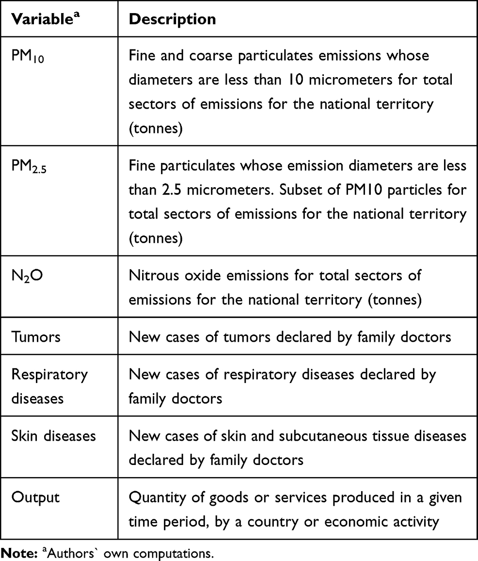Table 1 Description of the Variables

Figure 1 shows that during the 1995 to 2017 period, the number of new cases of tumours increased by +163.20%, while the number of new cases of respiratory and skin diseases decreased by 30% and −22.5%, respectively. Nitrous oxide emissions decreased by −6.66%, and PM₁₀ and PM_2.5 particle emissions increased by +29% and +58%, respectively. Furthermore, in the case of PM₁₀ and PM_2.5 particle emissions, more than half were generated by household activities (66.88% for PM₁₀, and 82.75% for PM_2.5 in 2017). Only for N₂O emissions, 96.63% of them were generated by economic activities in 2017. By comparison to EU statistics, daily concentration levels were exceeded for PM₁₀ in 19% of the surveillance stations, and in 6% of them for PM_2.5.²⁹ This tells us that the urban population of the European Union was exposed in 2015 to pollution levels by 19% above the upper ceiling in the case of PM₁₀, up from the previous year’s level), and by 7% above the upper limit, in the case of PM_2.5, down from the previous year’s level.²⁹

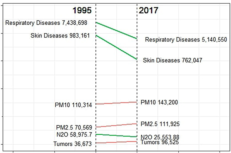Figure 1 Evolution of new diseases and air pollution emissions from 1995 to 2017.

Methodology

In this paper, we use three statistical methods for establishing links between air pollutants and different diseases, determining the size of the effect of the air pollutants on diseases and the factors generating air pollutants in Romania. The data accessed were freely available on Eurostat database (1995–2017) and from the National Institute of Statistics of Romania TEMPO. These methods are Toda-Yamamoto procedure of non-causality Granger test, grey relational analysis and logarithmic mean Divisia index method (LMDI). Our goals and the reasons we used these methods are explained in the overall framework represented in Figure 2.

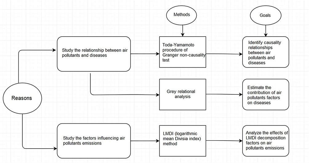Figure 2 Theoretical structure of methods.

Toda-Yamamoto Procedure of Granger Causality Test

In time series analysis, one useful and well-known method for measuring the degree of association between two variables is quantified by correlation tests. However, correlation does not necessarily imply causality. Hence, another statistical tool is needed and one such tool is Granger causality test that investigates causality between two variables. Causality in time-series analysis is useful in assessing if a variable is a factor, and thus provides useful information, in forecasting another variable. In this paper, we investigate the causality between air pollution emissions (PM₁₀, PM_2.5, N₂O) and different diseases (tumors, respiratory diseases and skin diseases). Even though air pollution have many more health implications, such as ischemic heart disease, stroke, diabetes and pre-term birth, due to availability of data we only considered a small subset of diseases represented by tumors, respiratory diseases and skin diseases. The statistical method used is Toda-Yamamoto procedure of Granger non-causality test since the latter requires stationary series which is problematic since unit-root and co-integration test accuracy depends on power and size properties potentially leading to incorrect results.³⁰ Hence, to overcome this problem, a solution is Toda-Yamamoto procedure of Granger non-causality test.³¹ The direction of causality can be one direction, both directions or neither. In this paper, we are only interested in asserting one direction causality, from air pollutants to diseases.

Toda-Yamamoto method estimates and fits a vector autoregression (VAR) model of order in order to minimise “the risks associated with possible incorrect identification of the order of integration of the series”.³² Hence, a first step is identification of the order of integration of the series. After this step, a VAR(p) model is fitted and the maximal order of integration is determined; a VAR model is estimated. The non-causality Granger analysis uses a modified Wald test of zero restrictions hypothesis (F-statistics) to assess the significance of the lagged values of on , after the VAR model is estimated. The Toda-Yamamoto approach ensures a chi-square ( asymptotic distribution for inference analysis.

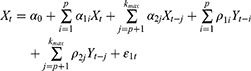
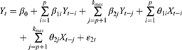
The VAR model of a model subject to Toda-Yamamoto version of the Granger non-causality test is given by:

(1)

(2)

Granger causality from to implies (Equation 1) while Granger causality form to implies .

The hypotheses tested are as follows:

Hypothesis 1 (H1): PM₁₀ does not Granger cause new cases of tumours.

Hypothesis 2 (H2): PM₁₀ does not Granger cause new cases of respiratory diseases.

Hypothesis 3 (H3): PM₁₀ does not Granger cause new cases of skin diseases.

Hypothesis 4 (H4): PM_2.5 does not Granger cause new cases of tumours.

Hypothesis 5 (H5): PM_2.5 does not Granger cause new cases of respiratory diseases.

Hypothesis 6 (H6): PM_2.5 does not Granger cause new cases of skin diseases.

Hypothesis 7 (H7): N₂O does not Granger cause new cases of tumours.

Hypothesis 8 (H8): N₂O does not Granger cause new cases of respiratory diseases.

Hypothesis 9 (H9): N₂O does not Granger cause new cases of skin diseases.

If the probability of any of the above hypothesis is less than the critical value of 0.05, then the hypothesis is rejected and as such Granger-causes , meaning is a factor to .

Grey Relational Analysis

To quantify the effect of each air pollutant factor on the tendency of each disease we perform a grey relational analysis (GRA) which is based on grey system theory developed and introduced by Deng in 1982.^33,34 GRA describes the relationship of size, intensity and order between variables reflecting the changing trend of those variables given by size, direction and speed. Grey relational analysis is a quantitative method based on similarity or dissimilarity between factors with application in determining the correlation degree of influencing factors.^33–35 It calculates a grey relational degree which can be easily interpretated. A large grey relational degree suggested a stronger correlation between variables and as such the sample data reflects the changing trend of the factors analyzed. GRA has low data requirements and little calculation work. The procedure of GRA analysis is as follows.

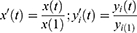
Let be the mother sequence while is the subsequence, where represents the time, . First step in grey relational analysis is applying a dimensionless method to the sequences either by mean value method or initial value method. The former method divides all values of the sequence to the mean value while the latter divides all values of the sequence to the first value.

In this paper, we apply the initial value method:

(3)

Grey relational coefficient between and at moment of time is:

(4)

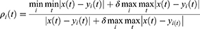
where is the distinguishing coefficient which is usually taken to be . Grey relational coefficient between and is:

(5)

Grey relational method analyses how close a relationship between two sequences is based on the degree of similarity of the sequence geometry. This technique does not require any assumptions about the distribution of the data. represents the degree of influence of on . Maximum value for grey relational degree is 1 indicating a great correlation. When , an obvious correlation is given by a value of of the grey relational coefficient. Moreover, if then variable has a greater effect on tendency of than .

Decomposition of Air Pollution Emissions Factors-LMDI Method

Factors influencing air pollutants emissions include reduction of energy consumption, renewable energy production and vehicle traffic intensity. In this paper, we investigated two factors that influence air pollutants emissions in Romania, namely technology improvements of economic activities and economic structural changes. The most important driver of air pollutants emissions is industry production and one way to improve air quality is using new and innovative technologies in the industry production and other economic sectors. However, Romania has gone through a deindustrialization process in the last decades and as such air pollution emission reduction can be mostly due to economic structural changes and not as a result of technology improvements.⁸ To quantify the effect of these two factors on air pollution emissions and to investigate which of these two factors has a bigger impact in reducing or increasing air pollutants we perform a logarithmic mean Divisia index method (LMDI).

LMDI method was introduced in 1998 by Ang and has been widely used in water pollution decomposition, industry, transport, energy, and other fields.^36–42 Some of its advantages include lack of residuals, ease of use, complete decomposition and, additive and multiplicative decompositions.⁴³ In this paper, a multiplicative decomposition is used as the results can be easily transformed in percentage points and therefore are easier to interpret. The LMDI method requires an aggregated index to decompose into factors. The LMDI procedure is as follows.

An aggregated index of total air pollution intensity (PM₁₀, PM_2.5, N₂O intensities) of the Romanian economy at time , denoted by , is defined, based on the existing literature, as a weighted average of sector air pollution intensities as follows:^44–47

(6)

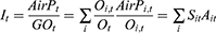
where is a period of time, represents the economic sector, is the air pollution emission produced by sector in period ; is the air pollution emission produced by the whole economy in period ; is output of sector in period ; is the output as a measure of economic activity in period ; is the share of sector in total output in period ; is the air pollution intensity of sector in period .

Changes in air pollution intensity can be due to structural changes in the economy (- structural effect) or changes in sector air pollution reduction strategy efficiency (- technology effect) given by changes in air pollution intensity.

We use the logarithmic mean Divisia index LMDI model based on Kaya identity to decompose the PM₁₀, PM_2.5, N₂O air pollution intensity of the Romanian economy. The method does not generate a residual term, the decomposition being perfect.

The multiplicative decomposition of changes in total air pollution intensity between the periods and is described by:

7

where is the estimated impact of structural change on total air pollution intensity in period , while is the estimated impact of changes in the sector air pollution intensity levels in period which can be explained by a change in the efficiency of the corresponding sector (technology effect), and is the total change of total air pollution intensity. These factors are given by:

(8)

(9)

where , being the natural logarithm; is the sector’s share of air pollution emissions within the economy. A value of for is interpreted as an increase of decrease of (depending on the sign) in the total air pollution intensity given by structural changes in the economy. and are interpreted similarly.

Results

This section is dedicated to results. Firstly, we present an overview of air pollution intensity developments in Romania over the 2008–2017 period. The Toda-Yamamoto procedure and grey relation analysis results are presented next. Lastly, LMDI decomposition results are discussed.

Air Pollution Intensity Developments

Air pollution emissions and intensity developments for economic activities for the 2008–2017 period are displayed in Tables 2 and 3, respectively. We notice that the emissions arising from economic activities have diminished during the period analyzed, with a considerable drop for PM_2.5. However, the fact that activities in the manufacturing, construction, and agriculture sectors diminished in intensity, while business in the services sector grew, did not necessarily reflect in the level of pollution. It was only in agriculture that emissions grew both in volume and intensity, despite a downward trend of farming activities. In the manufacturing sector, the output went up, and all the emissions of pollutants examined for the purposes hereof dropped in volume and intensity, which indicates the replacement of the highly polluting technologies by cleaner ones.

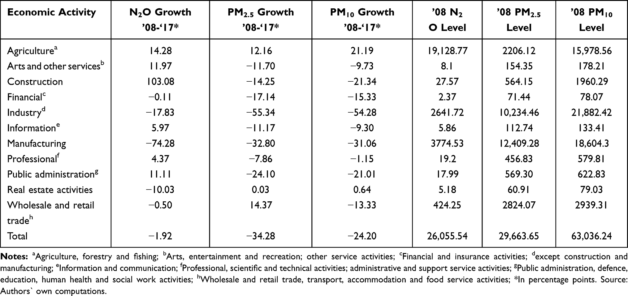Table 2 Growth Rates and Levels of Air Pollution Emission Developments in Romania

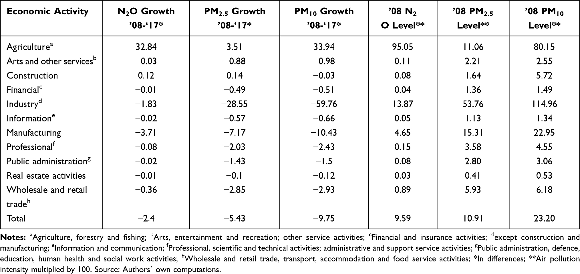Table 3 Growth Rates and Levels of Air Pollution Intensity Developments in Romania

To further examine the air pollutant emissions various violin distribution plots are displayed in Figures 3–9. Through these violin plots, the transformations in the economy, with respect to the volume and intensities of emissions, can be observed. Violin distribution is a special kind of visualizing data allowing us to see where the data are clustered, around the maximum/minimum values or around the median by showing peaks in the data. The wider the distribution in a value indicates highly concentrated values in that particular value. A violin plot is a hybrid between a kernel density plot and a box plot. The difference between a violin plot and a box plot is that the latter does not let you see variations in the data. The results of the violin plots are as follows.

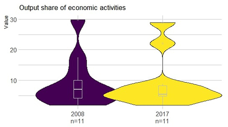Figure 3 Output share violin distribution and boxplot of economic activities in 2008 and 2017. Source: Authors` own computations.

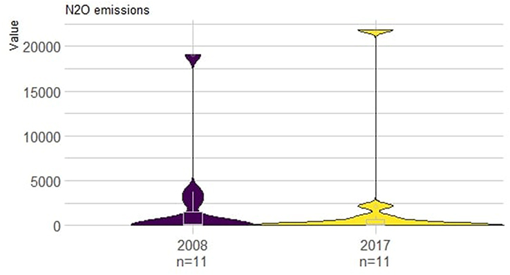Figure 4 N2O pollution emissions. Source: Authors’ own computations.

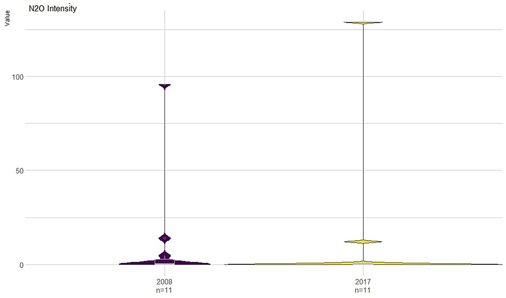Figure 5 N2O pollution intensity. Source: Authors’ own computations.

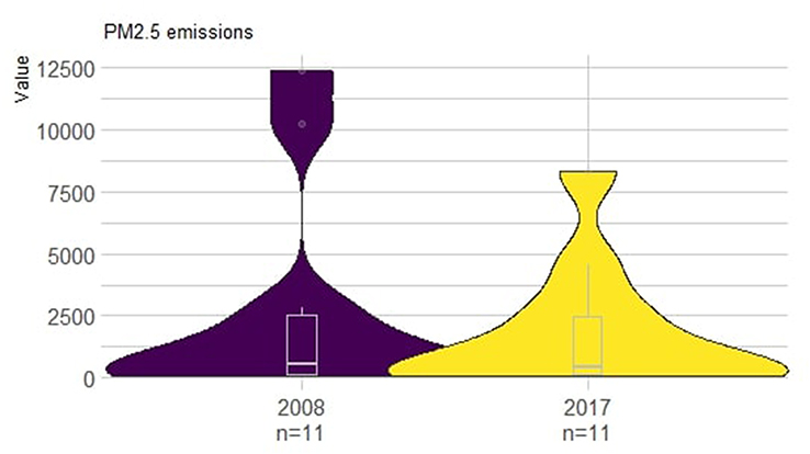Figure 6 PM2.5 pollution emissions. Source: Authors’ own computations.

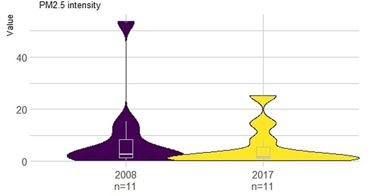Figure 7 PM2.5 pollution intensity. Source: Authors’ own computations.

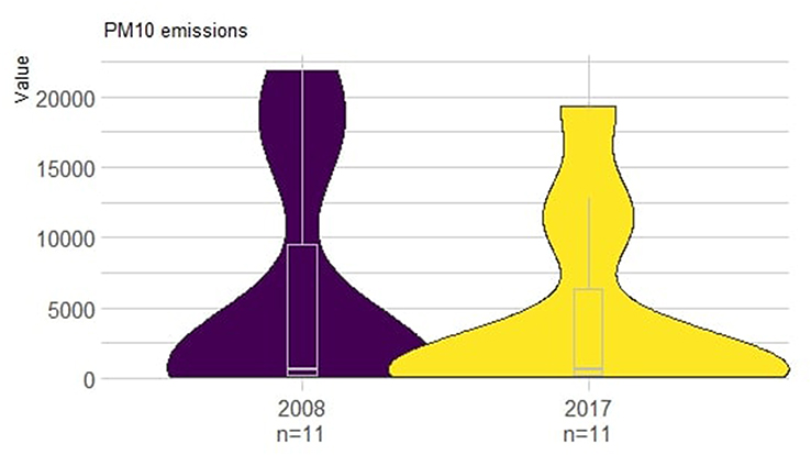Figure 8 PM10 pollution emissions. Source: Authors’ own computations.

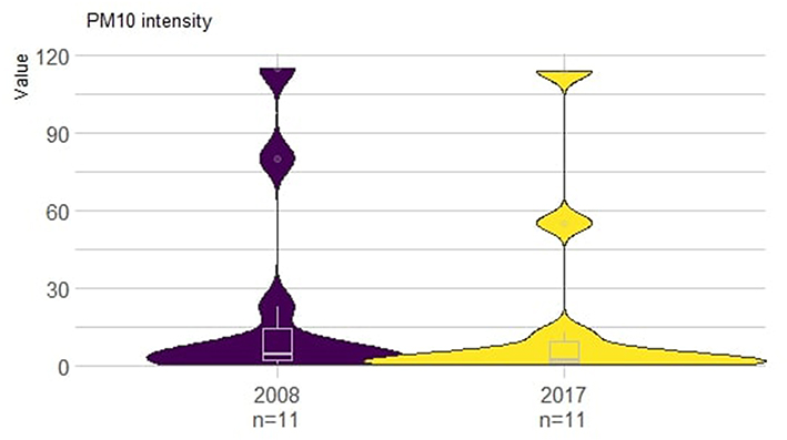Figure 9 PM10 pollution intensity. Source: Authors’ own computations.

First, we observe that most output shares of economic activities are situated around the median value in the lower part of the violin distribution for 2008 and 2017 (7% median in 2008, 5.38% median in 2017).

In Romania, holding the first three slots in the economy during the reference period were the manufacturing, wholesale and construction sectors. In 2017, the top three sectors were manufacturing, wholesale and public administration, which is proof that the Romanian economy shifted accent to the services sector. While in 2008 the share of business in the services sector was closer to the shares of the important economic sectors, in 2017 there is a visible gap between the lower and upper parts of the distribution, suggesting a wider polarization of output share of economic activities.

Furthermore, there are two parts in the upper violin distribution, the difference between manufacturing output share (maximum output share 28.82%), wholesale (second largest output share 22.06%) and public administration (third largest output share) being 19.97% and 13.21%, respectively.

N₂O pollution emissions in Romania are released heavily by the agriculture, forestry and fishing sector (Figure 4). The gap of N₂O emissions between agriculture and the other sectors has increased from 2008 to 2017. N₂O intensity in agriculture was the highest in 2008 and 2017 among all N₂O intensities (Figure 5).

PM_2.5 emissions are released mainly from industry and manufacturing activities. However, since industrial activities have decreased, the difference of emissions and intensities between other sectors and industries and the manufacturing sectors has diminished (Figure 6). PM_2.5 intensities have decreased from 2008 to 2017 for industry (over 50% decrease) and for manufacturing (by almost 50%) (Figure 7).

PM₁₀ emissions are released mainly from industry, manufacturing and agriculture activities. While in 2008 most PM₁₀ emissions were generated by industrial activities, followed by manufacturing, in 2017, most emissions were generated by agricultural activities, followed by manufacturing (Figure 8). PM₁₀ intensities for agriculture increased, while they decreased for industry and manufacturing by almost 50% (Figure 9).

As such, decline in industrial activities decreased air pollutant emissions in Romania; however, the biggest problem is represented by agricultural activities which show an increase in volume and intensity of N₂O and PM₁₀ emissions which could lead to potential health risks for individuals.

Toda-Yamamoto Procedure Results

Toda-Yamamoto procedure determines if an air pollutant is a factor for a disease and it is based on a Granger non-causality test. Before presenting the results of the procedure, some preliminary hypothesis needs to be tested and confirmed. Hence, the first step in Toda-Yamamoto procedure of Granger non-causality test is establishing whether the variables used in the analysis are integrated of order one. In Table 4 the results of the unit roots tests for series used in this study are displayed. We applied the Augmented Dickey-Fuller (ADF) and Kwiatkowski-Phillips-Schmidt-Shin (KPSS) tests. The null hypothesis of stationarity of the KPSS test is rejected when series in levels are taken into account considering a 5% critical value. However, when the first differences are taken, the null hypothesis of stationarity is accepted in all cases. At levels, the null hypothesis of non-stationarity of the ADF test cannot be rejected for all series, while at first differences the hypothesis is rejected in all cases, except for variable tumours. For this series, the hypothesis of non-stationarity is rejected at 10% critical value. Results show that all the variables considered (PM₁₀, PM_2.5, N₂O, Tumors, Respiratory diseases, Skin diseases) are integrated of order one. Hence, the maximal order of integration for all models of the Toda-Yamamoto Granger causality is . Next, the order of the VAR model on which the Granger non-causality test is based upon needs to be determined.

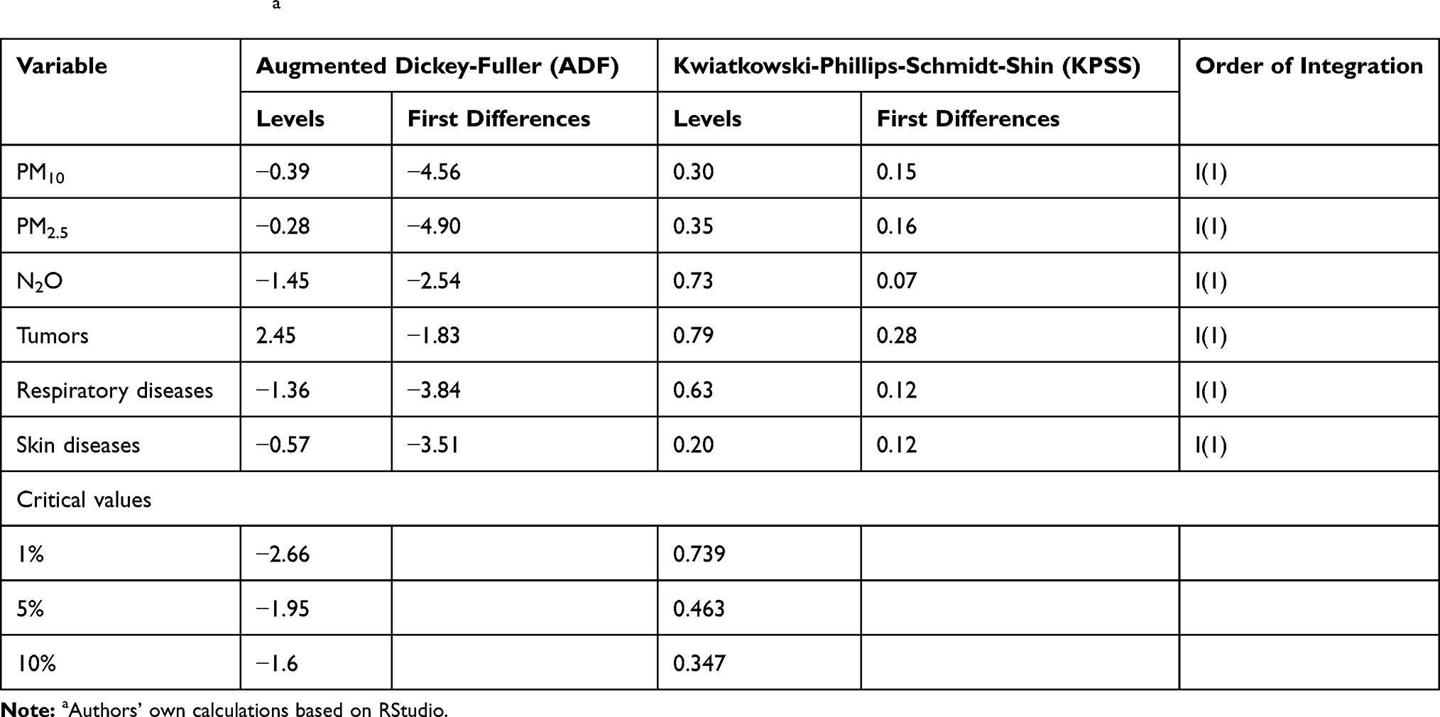Table 4 Unit Root Testsa

Order of VAR models is selected based on four information criteria: Akaike information criterion (AIC), Hannan-Quinn information criterion (HQ), Schwarz criterion (SC) and Final Prediction Error (FPE). If there is no clear value among the four information criteria, a decision is made based on the asymptotic Portmanteau test for autocorrelation, which biases the estimators making them less efficient. The next step is estimating the VAR model and performing the Granger non-causality test.

Rejection or acceptances of each of the nine hypotheses stated in a previous section is based on the modified Wald test. A probability lower than 0.05 rejects the non-Granger causality hypothesis which is what we are looking for. Table 5 presents the results for modified Wald test for Toda-Yamamoto version of Granger non-causality test. Out of the nine hypotheses, only three cannot be rejected. Hence, PM₁₀ particles do Granger cause new cases of tumours and respiratory diseases. The same being true for PM_2.5 particles. N₂O does Granger cause new cases of skin diseases and new cases of tumours.

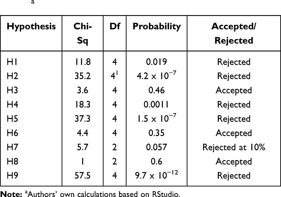Table 5 Toda-Yamamoto Version of Granger Causality Test Resultsa

Hence, PM₁₀ and PM_2.5 are factors for tumors and respiratory diseases, while N₂O is a factor for tumors and skin diseases.

Grey Relational Analysis Results

In the previous subsection, we established Granger causality relationships between air pollutants and different diseases. However, to see which air pollutant has a bigger impact on the three diseases considered in this study, a grey relational analysis is performed. As such, Table 6 contains the results of the grey relational analysis between diseases and air pollution emissions, for the 1995–2017 period.

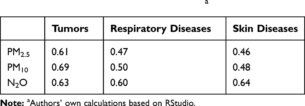Table 6 Grey Correlation Analysis Resultsa

New cases of tumours have a strong correlation with all three air pollutions (grey correlation coefficient is over 0.60). PM₁₀ has the most similar trend with new cases of tumours, followed by N₂O and PM_2.5. A strong correlation exists also between N₂O and new cases of respiratory and skin diseases. The second factor influencing these two diseases is PM₁₀, which has a weaker correlation as compared with N₂O. The least dominating behavior factor influencing respiratory and skin diseases is PM_2.5. As a first result, governmental policies addressing public health should firstly reduce air emissions of PM₁₀ and N₂O, to improve air quality and health of individuals.

Decomposition of Air Pollution Intensity Results

In order to better understand the causes and factors that influence the level of pollution generated by the three environmental variables chosen for the purposes hereof, we have applied the pollution intensity decomposition to each one of them. We have proceeded to the pollution intensity decomposition for: N₂O, PM_2.5 and PM₁₀. Table 7 contains the results of the decomposition of air pollution intensity.

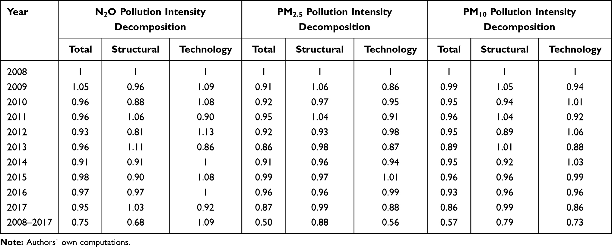Table 7 Decomposition of Air Pollution Intensity

A first result is that, on average, the structural changes in the economy have contributed to an annual decreasing rate of 3.45% of the N₂O emission intensities in the reference period 2008–2017, but the changes of intensities by type of economic activity (accounted for by newer, less polluting know-how) increased the intensities, on average, by 1.15% per year. The overall intensity of N₂O emissions (defined as N₂O emission per economic output, in tonnes/million euro) during 2008–2017 went down by 24.97%, to which the structural changes in the economy contributed by −31.18%, while the know-how transformations (reflected in intensities) contributed by + 9.032%.

Structural changes in the economy contributed a reduction of 1% per year of the intensity of PM_2.5 emissions; the changes of intensity by economic activity contributed by an average of −11.22%. Over the entire period 2008–2017, the intensity of PM_2.5 dropped by 49.72%, the structural changes in the economy contributed a reduction of 11.25%, while technological upgrading reduced intensities by 43.34%.

The structural changes in the economy contributed to the decrement of intensity of PM₁₀ emissions by 2.23% in each of the years of the reference period 2008–2017; the changes in the intensities of the various economic activities contributed an average reduction of 3.39% per year. For the overall period 2008–2017, the intensity of PM₁₀ dropped by 42.01%, the structural changes in the economy contributed by −20.86%, while the new technologies contributed by −26.73% intensity-wise.

In Figure 10 one can see the dynamics of the evolution of the effects and influences of the development and restructuring in Romania’s national economy from the perspective of the decomposition of the main air pollution intensity components – taking the year 2008 as reference.

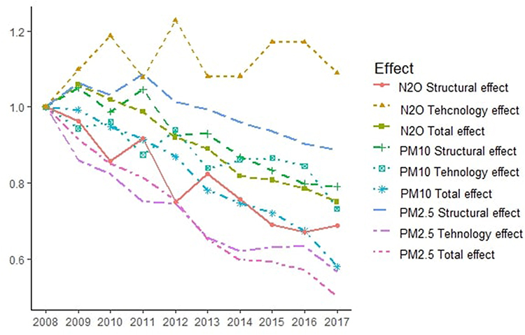Figure 10 Evolution of the decomposition of the main air pollution intensity components.

Discussion and Conclusions

The findings of this study have revealed a significant relationship between air pollution and various diseases for Romania. Among the three air pollutants, considered in this study, PM₁₀ and PM_2.5 are factors and have a significant relationships for tumors and respiratory diseases, while N₂O is a factor for tumors and skin diseases. The significant relationship between tumors and all three air pollutants is also confirmed by the grey relational analysis which showed a strong correlation degree between air pollutants and tumors revealing an order of factors according to the size of impact on the number of tumours as PM₁₀> N₂O > PM_2.5. There is also a strong correlation degree between N₂O and skin diseases. The main sources of PM₁₀ emissions are industry, manufacturing and agriculture activities. During the 2008–2017 period, we notice a shift of PM₁₀ emissions main source from industry to agricultural. PM₁₀ intensities have significantly decreased for industry and manufacturing by almost 50%, while for agriculture increased by 42%. The main source of N₂O emissions is agricultural, forestry and fishing activities. The main sources of PM_2.5 emissions are industry and manufacturing. However, PM_2.5 intensities have dropped significantly from 2008 to 2017 by approximately 50% in both economic activities. Hence, PM₁₀ and N₂O emissions have as common main source agriculture.

LMDI decomposition revealed that air pollutants intensities dropped over the 2008–2017 period due to structural changes in the economy (in case of N₂O and PM₁₀ with over 20%). Only in case of PM_2.5 the intensities dropped significantly due to technology changes. In case of N₂O, technology used increased the air pollutant intensity. The cause of this is agricultural practices which in the last decades intensified the use of chemical fertilizers which increased by 46% while quantity of insecticide used grew by 18%. While other economic activities reduced their emissions due to technology changes, agriculture remains the only economic activity which lacks technology improvements. Organic agriculture produces with 40.2% less N₂O emissions per hectare than non-organic systems.⁴⁸ However, without government control and effective support, organic agriculture is poorly developed in Romania. The percentage of total utilized agricultural area of total fully converted and under conversion to organic farming of utilized agricultural area excluding kitchen gardens was 1.93% in 2017 for Romania, while at the European Union level was 7.03%. Other factors generating air pollutants from agriculture are livestock activities, manure management and burning of crop residuals.

We have seen that during 2008–2017 period in was only in agriculture that air pollutant emissions grew both in volume and intensity, despite a downward trend of farming activities output. Without government intervention agricultural activities will effect even further not only the air but also the land, leading to land degradation and health problems. Given the results of this paper, air quality and health policy in Romania should first address agricultural activities.

Agriculture activities in Romania are supported through the Common Agricultural Policy of the European Union being an important support for organic agriculture which allowed thousands of farmers to get organic agriculture certifications. State authorities support organic agriculture through incentives in form of payments in euro per hectare, training programs and promoting local farmers. Even though farmers who have a minimum farm area of 1 hectare are eligible for financial support, the average size of an organic farm is 72 hectares for field crops and 42 hectares for permanent crops.⁴⁹ Moreover, most organic farming is performed by large farms (over 100 hectares) or medium-sized farms (10–100 hectares).⁴⁹ Only a small share of subsistence and semi-subsistence farms (1–10 hectares) practice organic agriculture. Subsistence and semi-subsistence farms account for 40.4% of the land and represent 42.2% of the total farmers.⁵⁰ The reason for this situation is that these type of farmers produce primarily for their own food consumption and use and as such they are less interested in the organic product market and selling their products at a bigger price. Currently, the agricultural policy does not address separately the needs, characteristics and motivations of the smaller farmers from those of the bigger farmers.

Other options for mitigating agricultural air pollution are investigated by Fellman et al (2018).⁵¹ They showed that change in livestock production management has a rather limited effect in reducing emissions and proposed a solution of adjusting the quantity of production. Moreover, in developing countries as Romania, technology improvement options are important for mitigation of agricultural emissions. A recent study shows that there is a strong relationship between intensive crops, livestock activities and agricultural carbon emissions.⁵²

Government policy makers should address the agricultural emissions by taking into account the characteristics of the Romanian agriculture which is highly polarized with subsistence and semi-subsistence farms owning almost half of the land and their motivation being different from the motivation of larger farmers.^50,53 Due to this polarization, health policy regarding agricultural emissions requires substantial incentives and support measures. These measures can take the form of training of farmers (with the support of local authorities) or investment support for using new cleaner production technology in agriculture. Another aspect to take into account by policy makers is the energy-related air pollutants. Yan et al (2017) showed that in Romania that energy-related greenhouse gas emission generated by agricultural activities were affected by decrease of energy use and not as a consequence of a better and efficient management of agricultural production based on energy-efficient technology.⁵⁴ Hence, policy makers should also address this issue by encouraging and stimulating the use of more energy-efficient technology and renewable energy.

References

1. Năstase G, Șerban A, Năstase AF, Dragomir G, Brezeanu AI. Air quality, primary air pollutants and ambient concentrations inventory for Romania. Atmos Environ. 2018;184:292–303. doi:10.1016/j.atmosenv.2018.04.034
2. Mitsakou C, Dimitroulopoulou S, Heaviside C, et al. Environmental public health risks in European metropolitan areas within the EURO-HEALTHY project. Sci Total Environ. 2019;658:1630–1639.
3. Bayat R, Ashrafi K, Motlagh MS, et al. Health impact and related cost of ambient air pollution in Tehran. Environ Res. 2019;176:108547. doi:10.1016/j.envres.2019.108547
4. Likhvar VN, Pascal M, Markakis K, et al. A multi-scale health impact assessment of air pollution over the 21st century. Sci Total Environ. 2015;514:439–449. doi:10.1016/j.scitotenv.2015.02.002
5. Hankey S, Marshall JD. Urban form, air pollution, and health. Curr Environ Health Rep. 2017;4(4):491–503. doi:10.1007/s40572-017-0167-7
6. Oncioiu I, Dănescu T, Popa MA. Air-pollution control in an emergent market: does it work? Evidence from Romania. Int J Environ Res Public Health. 2020;17(8):2656. doi:10.3390/ijerph17082656
7. Dragomir MCB, Munteniță C, Simionescu AG, Zeca DE, Kramar I, Marynenko N. Seasonal and spatial variation of PM10 in an urban area from Romania. J Vasyl Stefanyk Precarpath Nat Univ. 2019;6(3–4):7–14. doi:10.15330/jpnu.6.3-4.7-14
8. Chivu L, Constantin C, George G. Deindustrialization and Reindustrialization in Romania. Palgrave Macmillan; 2017.
9. Bergamaschi R, Cortese A, Pichiecchio A, et al. Air pollution is associated to the multiple sclerosis inflammatory activity as measured by brain MRI. Mult Scler. 2018;24(12):1578–1584. doi:10.1177/1352458517726866
10. Neamtiu IA, Lin S, Chen M, Roba C, Csobod E, Gurzau ES. Assessment of formaldehyde levels in relation to respiratory and allergic symptoms in children from Alba County schools, Romania. Environ Monit Assess. 2019;191(9):1–11. doi:10.1007/s10661-019-7768-6
11. Levei L, Hoaghia MA, Roman M, et al. Temporal trend of PM10 and associated human health risk over the past decade in Cluj-Napoca city, Romania. Appl Sci. 2020;10(15):5331. doi:10.3390/app10155331
12. Ambient (outdoor) air pollution. World Health Organization; 2016. Available from: https://www.who.int/news-room/fact-sheets/detail/ambient-(outdoor)-air-quality-and-health.
13. Chen F, Chen Z. Cost of economic growth: air pollution and health expenditure. Sci Total Environ. 2020;755:142543.
14. World Bank. Cost of Pollution in China. Washington DC: World Bank; 2007.
15. Fauser P, Ketzel M, Becker T, et al. Human exposure to carcinogens in ambient air in Denmark, Finland and Sweden. Atmos Environ. 2017;167:283–297. doi:10.1016/j.atmosenv.2017.08.033
16. Janke K. Air pollution, avoidance behaviour and children’s respiratory health: evidence from England. J Health Econ. 2014;38:23–42. doi:10.1016/j.jhealeco.2014.07.002
17. Ebenstein A, Lavy V, Roth S. The long-run economic consequences of high-stakes examinations: evidence from transitory variation in pollution. AEJ Appl Econ. 2016;8(4):36–65.
18. World Health Organization. Ambient air pollution - a major threat to health and climate. 2018. Available from: https://www.who.int/airpollution/ambient/en/.
19. Rajak R, Chattopadhyay A. Short and long-term exposure to ambient air pollution and impact on health in India: a systematic review. Int J Environ Health Res. 2019;30:1–25.
20. Heyes A, Zhu M. Air pollution as a cause of sleeplessness: social media evidence from a panel of Chinese cities. J Environ Econ Manage. 2019;98:102247. doi:10.1016/j.jeem.2019.07.002
21. Varvarigos D. Environmental degradation, longevity, and the dynamics of economic development. Environ Resour Econ. 2010;46(1):59–73. doi:10.1007/s10640-009-9334-0
22. Chakraborty S. Endogenous lifetime and economic growth. J Econ Theory. 2004;116(1):119–137. doi:10.1016/j.jet.2003.07.005
23. Liu F, Zheng M, Wang M. Does air pollution aggravate income inequality in China? An empirical analysis based on the view of health. J Clean Prod. 2020;271:122469. doi:10.1016/j.jclepro.2020.122469
24. Cheng Z, Jiang J, Fajardo O, Wang S, Hao J. Characteristics and health impacts of particulate matter pollution in China (2001–2011). Atmos Environ. 2013;65:186–194. doi:10.1016/j.atmosenv.2012.10.022
25. Charafeddine R, Boden LI. Does income inequality modify the association between air pollution and health? Environ Res. 2008;106(1):81–88. doi:10.1016/j.envres.2007.09.005
26. Eurostat database. Environment (1995–2017). Available from: https://ec.europa.eu/eurostat/web/environment/data/database.
27. National Institute of Statistics of Romania. TEMPO online database; 2020. Available from: http://statistici.insse.ro:8077/tempo-online/#/pages/tables/insse-table.
28. Sivarethinamohan R, Sujatha S, Priya S, Gafoor A, Rahman Z. Impact of air pollution in health and socio-economic aspects: review on future approach. Mater Today Proc. 2020.
29. European Union. Communication from The Commission to The European Parliament, The Council, The European Economic And Social Committee And The Committee Of The Regions A New Skills Agenda For Europe Working together to strengthen human capital, employability and competitiveness {SWD(2016) 195 final}, Brussels, 2016. Available from: https://eur-lex.europa.eu/legal-content/en/TXT/?uri=CELEX%3A52016DC0381. Accessed September 12, 2020.
30. Zapata HO, Rambaldi AN. Monte Carlo evidence on cointegration and causation. Oxf Bull Econ Stat. 1997;59(2):285–298. doi:10.1111/1468-0084.00065
31. Toda HY, Yamamoto T. Statistical inference in vector autoregressions with possibly integrated processes. J Econom. 1995;66(1–2):225–250. doi:10.1016/0304-4076(94)01616-8
32. Mavrotas G, Kelly R. Old wine in new bottle: testing causality between savings and growth. Manchester Sch Suppl. 2001;69(s1):97–105. doi:10.1111/1467-9957.69.s1.6
33. Deng J. Introduction to grey system theory. J Grey Syst. 1989;1(1):1–24. Chinese.
34. Deng J. Introduction to Grey Mathematical Resource Science. Wuhan, China: Huazhong University of Science & Technology Press; 2010. Chinese.
35. You ML, Shu CM, Chen WT, Shyu ML. Analysis of cardinal grey relational grade and grey entropy on achievement of air pollution reduction by evaluating air quality trend in Japan. J Clean Prod. 2017;142:3883–3889. doi:10.1016/j.jclepro.2016.10.072
36. Ang BW, Zhang FQ, Choi KH. Factorizing changes in energy and environmental indicators through decomposition. Energy. 1998;23(6):489–495. doi:10.1016/S0360-5442(98)00016-4
37. Lei H, Xia X, Li C, Xi B. Decomposition analysis of wastewater pollutant discharges in industrial sectors of China (2001–2009) using the LMDI I method. Int J Environ Res Public Health. 2012;9(6):2226–2240. doi:10.3390/ijerph9062226
38. Liang Y, Niu D, Wang H, Li Y. Factors affecting transportation sector CO2 emissions growth in China: an LMDI decomposition analysis. Sustainability. 2017;9(10):1730. doi:10.3390/su9101730
39. Yang X, Wang S, Zhang W, Li J, Zou Y. Impacts of energy consumption, energy structure, and treatment technology on SO2 emissions: a multi-scale LMDI decomposition analysis in China. Appl Energy. 2016;184:714–726. doi:10.1016/j.apenergy.2016.11.013
40. Zhang W, Li K, Zhou D, Zhang W, Gao H. Decomposition of intensity of energy-related CO2 emission in Chinese provinces using the LMDI method. Energy Policy. 2016;2016(92):369–381. doi:10.1016/j.enpol.2016.02.026
41. Zhao X, Song L, Tan S. Research on influential factors of agricultural carbon emission in Hunan province based on LMDI model. Environ Sci Technol. 2018;41(1):177–183.
42. Wen Y, Ceng K, Lei B, Zhou Y. Study on the influencing factors of agricultural carbon emission in Sichuan based on LMDI decomposition technology. IOP Conf Ser Mater Sci Eng. 2019;592(1):12179. doi:10.1088/1757-899X/592/1/012179
43. Ang BW. The LMDI approach to decomposition analysis: a practical guide. Energy Policy. 2005;33(7):867–871. doi:10.1016/j.enpol.2003.10.010
44. Zhao C, Chen B. Driving force analysis of the agricultural water footprint in China based on the LMDI method. Environ Sci Technol. 2014;48(21):12723–12731. doi:10.1021/es503513z
45. Xiong C, Yang D, Huo J. Spatial-temporal characteristics and LMDI-based impact factor decomposition of agricultural carbon emissions in Hotan Prefecture, China. Sustainability. 2016;8(3):262. doi:10.3390/su8030262
46. Lin Y, Yang J, Ye Y. Spatial–temporal analysis of the relationships between agricultural production and use of agrochemicals in eastern China and related environmental and political implications (based on decoupling approach and LMDI decomposition analysis). Sustainability. 2018;10(4):917. doi:10.3390/su10040917
47. Voigt S, De Cian E, Schymura M, Verdolini E. Energy intensity developments in 40 major economies: structural change or technology improvement? Energy Econ. 2014;41:47–62. doi:10.1016/j.eneco.2013.10.015
48. Skinner C, Gattinger A, Krauss M, et al. The impact of long-term organic farming on soil-derived greenhouse gas emissions. Sci Rep. 2019;9(1):1–10. doi:10.1038/s41598-018-38207-w
49. Popovici EA, Grigorescu I, Mitrică B, Mocanu I, Dumitraşcu M. Farming practices and policies in shaping the organic agriculture in Romania. A showcase of southern Romania. Rom Agric Res. 2018;35:163–175.
50. Feher A, Goșa V, Raicov M, Haranguș D, Condea BV. Convergence of Romanian and Europe Union agriculture–evolution and prospective assessment. Land Use Policy. 2017;67:670–678. doi:10.1016/j.landusepol.2017.06.016
51. Fellmann T, Witzke P, Weiss F, et al. Major challenges of integrating agriculture into climate change mitigation policy frameworks. Mitig Adapt Strateg Glob Chang. 2018;23(3):451–468. doi:10.1007/s11027-017-9743-2
52. Istudor N, Ion RA, Petrescu IE, Hrebenciuc A. Agriculture and the twofold relationship between food security and climate change. Evidence from Romania. Amfiteatru Econ. 2019;21(51):285–293.
53. Ciutacu C, Chivu L, Andrei JV. Similarities and dissimilarities between the EU agricultural and rural development model and Romanian agriculture. Challenges and perspectives. Land Use Policy. 2015;44:169–176. doi:10.1016/j.landusepol.2014.08.009
54. Yan Q, Yin J, Baležentis T, Makutėnienė D, Štreimikienė D. Energy-related GHG emission in agriculture of the European countries: an application of the Generalized divisia index. J Clean Prod. 2017;164:686–694. doi:10.1016/j.jclepro.2017.07.010
© 2021 The Author(s). This work is published and licensed by Dove Medical Press Limited. The
full terms of this license are available at https://www.dovepress.com/terms
and incorporate the Creative Commons Attribution
- Non Commercial (unported, 3.0) License.
By accessing the work you hereby accept the Terms. Non-commercial uses of the work are permitted
without any further permission from Dove Medical Press Limited, provided the work is properly
attributed. For permission for commercial use of this work, please see paragraphs 4.2 and 5 of our Terms.