Automated data-adaptive analytics for electronic healthcare data to study causal treatment effects

Introduction

Longitudinal health care databases are readily available and the most frequently used data source for studying the effectiveness of medical products in clinical care.^1–3 Along with randomized controlled trials (RCTs), regulatory agencies are increasingly integrating such database analyses into their decision making for drug approval and monitoring of unintended harm. Much has been done to improve our understanding of nonrandomized study designs in health care databases.^4,5 They have led to a number of studies that influenced how care is provided, including successful reproductions of RCTs,^6,7 successfully predicted findings from follow-on RCTs,^8,9 and changes in clinical practice where experimental studies were not feasible.^10,11 However, similar to the limited reproducibility of RCTs,¹² there are also many examples of misleading results from database studies in leading medical journals.^13–15 The lack of randomization and poorly designed studies have led decision makers to negative generalizations about the entire field of health care database research rather than a differentiated view of what is actionable evidence and what is not.¹⁶

Confounding that results from treatment selection based on outcome risk is well known to cause bias^17–19 and is generally most pronounced when studying intended treatment effects, comparing active treatment against untreated subjects²⁰ or comparing two different treatment modalities.²¹ Researchers recognized that the paucity of precision-measured confounder information in health care databases could be counteracted by utilizing those databases’ high-dimensional covariate space. High-dimensional propensity score (HDPS) approaches were the first to utilize such data for improved confounding adjustment and quickly gained popularity.^22,23 Their appeal stems equally from the ability to maximize confounding control with the available information from a given data source and the scalability through automated and optimized confounding adjustment that is data source independent.

This article reviews the current uses of HDPS, its performance across a variety of applications and data sources, its performance in simulation studies, and its current extensions using machine-learning techniques and other statistical learning strategies. The article is focused on analyses of health care databases and aims to provide specific and actionable advice, while drawing on generalized automated approaches to causal inference.

Working with longitudinal health care data to study treatment effects

Health care databases are derived from transactional databases that collect clinical and administrative information for the purpose of delivering and administering health care.²⁴ As encounters occur and services are provided, records are generated and added to an ever-growing database.³ Each addition comes with a service date stamp and is connected to the patient via a unique patient ID number, generating longitudinal patient records of increasing duration (Figure 1A). Individual entries may be delayed because bills are submitted late or due to administrative lag time, and retroactive changes may be made to correct a false entry related to services provided months in the past. There is substantial literature on the details of data integration, data cleaning, and data normalization, which will not be reviewed here.^25–27 As a first step to implement a study, one identifies and sets aside a section of the dynamic data stream that will cover the calendar time window of interest (Figure 1B). This stabilizes the data, a prerequisite for making results from a study of causal relationships replicable at a later point. In a prospective monitoring system, users may choose to freeze a data cut, including the most recent data, every time the data refresh. We now have an enumerable set of longitudinal patient records, each with a start date and an end date in calendar time. Encounters and services are recorded with diagnostic and procedural information on each patient’s individual time line (Figure 1C). The rules and algorithms that define a specific study design implementation will be applied to each patient’s longitudinal data stream (Figure 1D).

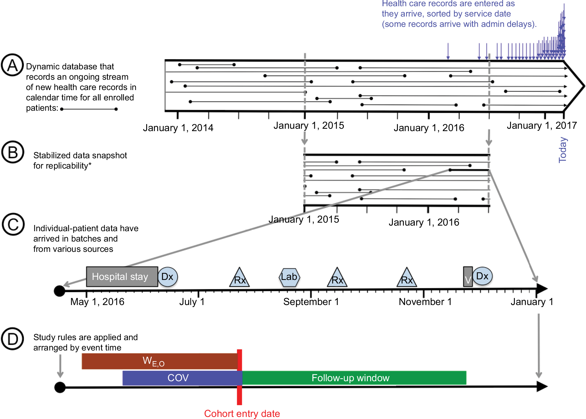Figure 1 From transactional data to study implementation. Notes: *Stabilization of dynamic data streams is critical if replicability of findings is important. In prospective monitoring systems with repeat analyses, one may want to stabilize data every time the source data are refreshed and analyzed. Abbreviation: COV, covariate assessment window.

In contrast to primary data collection, many measurements in health care databases (eg, patient baseline characteristics) are measured by reviewing information recorded during multiple health care encounters over a period of time. In primary data collection, a study subject’s health state is usually established when the patient is thoroughly interviewed or examined at a study visit. In health care databases, there is no defined interview date with the investigator team; studies rely instead on routine visits, and other health care encounters to collect information recorded during the provision of care. Several key concepts in epidemiological study designs that are assigned to specific points in time, eg, baseline patient characteristics before the start of exposure, are recorded over a period of time and reflect any encounters that occurred during that time window. In this article, we define a covariate assessment period (CAP) that starts at a defined number of days prior to cohort entry and ends at the beginning of exposure (Figure 2).²⁸

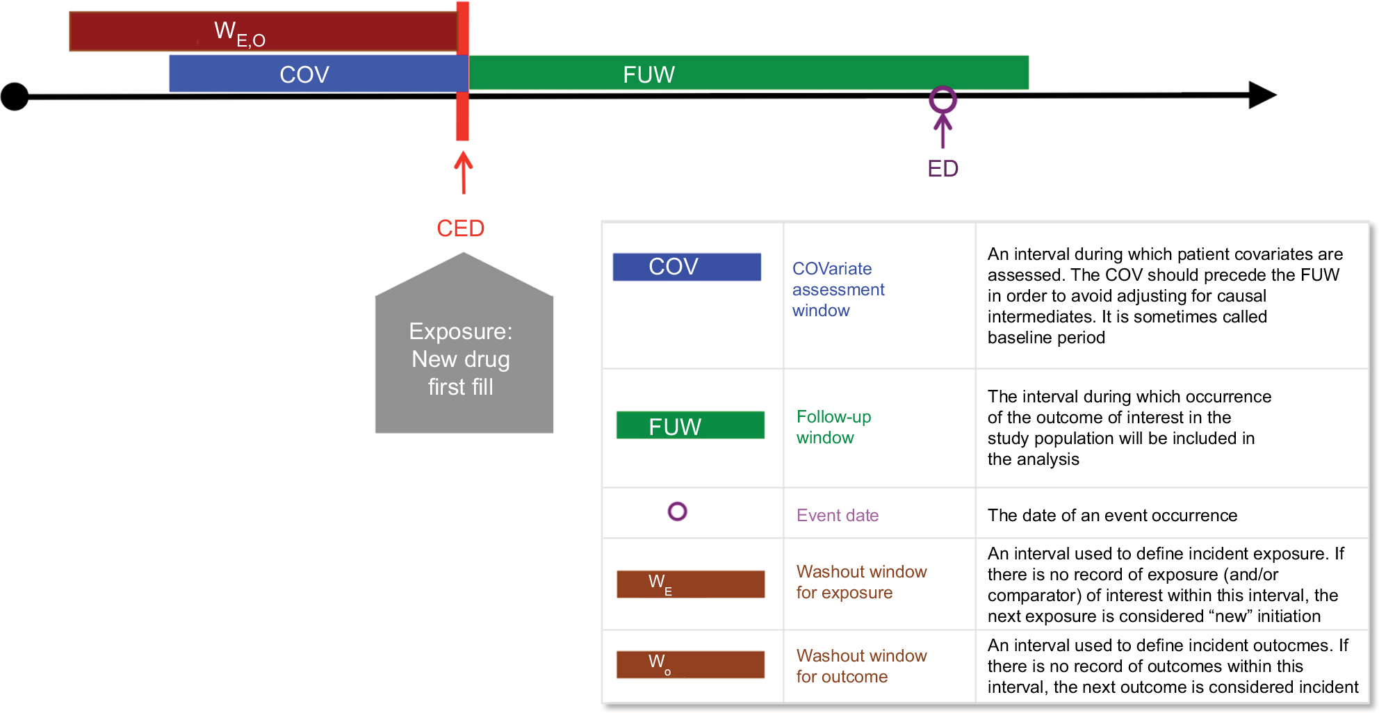Figure 2 Implementing causal analyses in longitudinal databases: a new-user cohort study. Notes: CED is on the day of initiation of the study exposure or comparison. The COV includes the date of the first fill in this example. Example: ACE inhibitors vs ARB and risk of severe angioedema. Data from Toh et al.116 Abbreviations: CED, cohort entry date.

Principles of high-dimensional proxy adjustment

The high-dimensional covariate space of longitudinal health care data

Any patient information recorded during the CAP can be considered to identify confounding factors. Since the optimal measurement of these factors is not in the investigator’s control, a key approach to reduce residual confounding from unobserved factors is to measure proxies of the underlying confounders (Figure 3). To the extent such proxy measurements are correlated with the underlying confounders, the unobserved confounders are measured and then adjusted.^29,30 Examples of well-measured proxies are the use of oxygen canisters (correlated with frail health) and the regular use of preventative services (correlated with health-seeking behavior) (Figure 3).

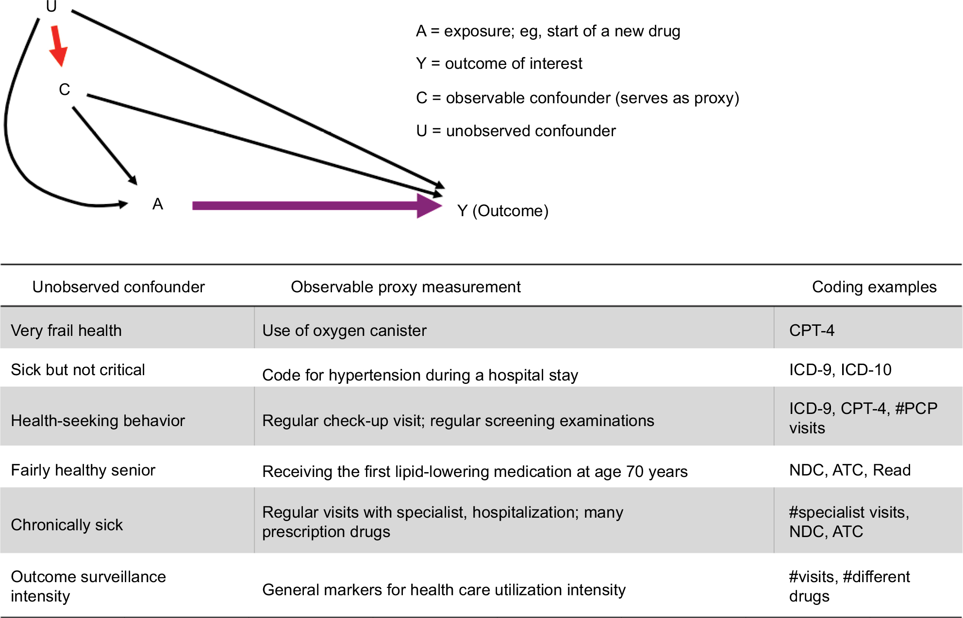Figure 3 Proxy measures of unobserved confounders as the principal reason for high-dimensional covariate adjustment. Abbreviations: ATC, Anatomical Therapeutic Classification; CPT, Current Procedure Terminology; ICD, International Classification of Disease; NDC, National Drug Code; PCP, primary care physician.

Proxies can be efficiently generated by turning codes that were recorded during the CAP into variables. In order to keep information of varying quality and interpretation separate, one wishes to define data dimensions of fairly homogeneous interpretation, such as diagnoses vs procedures and inpatient diagnoses vs outpatient diagnoses (Figure 4). For each such generated variable, additional attributes can be assigned, including how frequently the code is recorded within a CAP and the time elapsed between the code and the initiation of the exposure.³¹ Specific settings may require adding specific data dimensions, eg, staging and biomarker information in oncology or functional status measurements in musculoskeletal diseases. Together, this results in high-dimensional covariate spaces with several thousand covariates, some of which are confounders.

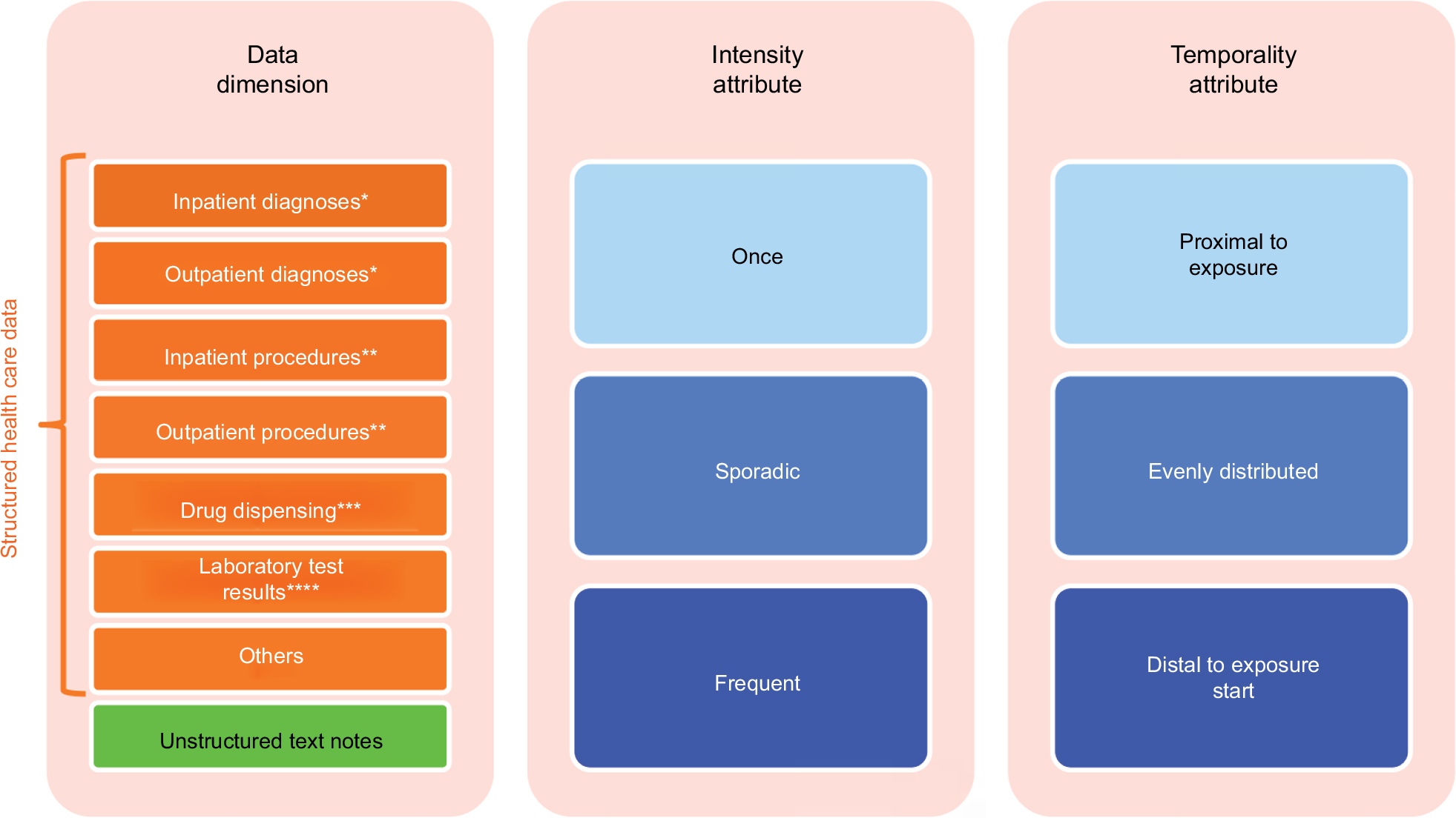Figure 4 Data characteristics containing covariate information in longitudinal health care databases. Notes: *Coding example: ICD. **Coding example: CPT. ***Coding examples: NDC and ATC. ****Coding example: LOINC. Abbreviations: ATC, Anatomical Therapeutic Classification; CPT, Current Procedure Terminology; ICD, International Classification of Disease; LOINC, Logical Observation Identifiers Names and Codes; NDC, National Drug Code.

The HDPS algorithm

The principles of high-dimensional covariate adjustment in database research can be divided into the following three steps: 1) automated covariate identification, 2) automated covariate prioritization, and 3) causal treatment effect estimation using propensity score (PS) analyses (Figure 5).^22,32

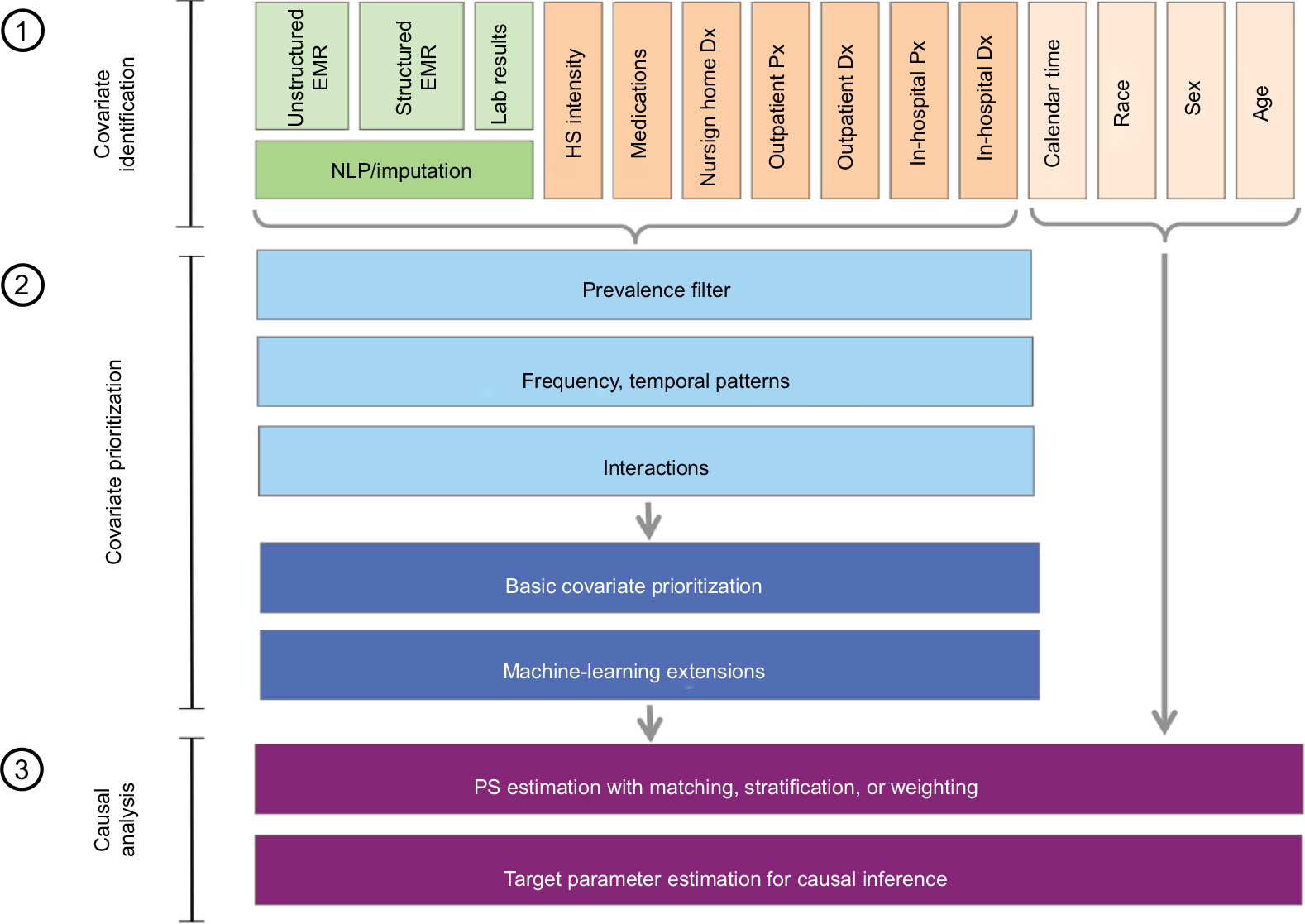Figure 5 Principles of high-dimensional covariate adjustment for estimating the following causal treatment effects: 1) automated covariate identification, 2) automated optimized covariate prioritization, and 3) causal treatment effect estimation using propensity score analyses. Abbreviations: NLP, natural language processing; Dx, diagnosis; Px, procedure; PS, propensity score.

Automated covariate identification

Health care databases can be divided into data dimensions, each containing a distinct subset of information of varying quality and often with specific coding systems, eg, inpatient diagnoses (5-digit International Classification of Disease [ICD] codes), outpatient procedures (5-digit Current Procedure Terminology [CPT] codes), and outpatient pharmacy drug dispensing (generic drug name). The HDPS algorithm considers distinct codes in each dimension without needing to understand their medical meaning and creates binary variables indicating the presence of each code/factor during a defined pre-exposure CAP.²² The basic HDPS version considered only the 200 most prevalent codes in each data dimension and for each code created three binary variables, indicating at least one occurrence of the code, sporadic occurrences, and many occurrences during the CAP;²² any of these parameters may be varied, and in fact, it has been argued that the prevalence filter may not be necessary.³³ All variables automatically created from health care databases are called “empirical” variables. With, say, five data dimensions, including inpatient diagnoses, inpatient procedures, outpatient diagnoses, outpatient procedures, pharmacy dispensing, and the HDPS, this would create up to 200×3×5=3000 binary variables. There can be more data dimensions, including laboratory test results, biomarker status, and free text, and more variables in each dimension, leading to substantially larger numbers of candidate variables. The variable-generating algorithm is agnostic to the medical meaning of each code and, therefore, can be applied to any structured or unstructured data source and coding systems.

Automated covariate prioritization

The key to successful confounding adjustment with propensity scores is to control for all risk factors of the outcome even if they are seemingly unrelated to treatment choice.^34–36 The HDPS algorithm reduces a large number of candidate covariates by prioritizing covariates for inclusion in a propensity score (PS) proportional to their association (relative risk [RR]) with the study outcome (RR_CD) and exposure (RR_CE). Epidemiology theory is quite clear on the fact that propensity score models should include all baseline predictors of the health outcome of interest even if they are only weakly or not at all associated with the exposure.^34–37 A propensity score model including all 3000 variables from the above example without any selection may not be estimable with standard logistic regression and may lead to inefficiencies due to collinearity and bias amplification by including instrumental variables.³⁶ Therefore, a heuristic technique determines which of the variables are likely the most important to include in the propensity score model. A simple yet effective covariate prioritization ranking, “bias ranking”, is well established. It selects the variables with the greatest potential to adjust for confounding using a formula by Bross that depends on the observed associations between covariates and outcome (RR_CD) and covariate and exposure (RR_CE).^22,38 The base-case assessed these associations in a bivariate way without further adjustment and selects the 500 top-ranked variables. Many other covariate prioritization strategies are available including those not considering the study endpoint.³⁹ After covariates have been prioritized and entered into a propensity score model using logistic regression, it is strongly recommended to also include patient attributes such as age, sex, and race and health service utilization variables such as number of visits and number of drug prescriptions filled.^39,40

Causal treatment effect estimation

Steps 1 and 2 yield long lists of prioritized covariates, which can now be used to minimize confounding through statistical analyses. Parametric and regularized outcome regressions have been recognized to have inadequate confounding adjustment when covariates are abundant and outcomes are rare.^41,42 However, propensity scores have the useful ability to reduce a large number of covariates into a single score and perform well in such settings.^34,43 PS matching is popular in most settings because of its analytic transparency and excellent performance;⁴⁴ PS (fine) stratification is recommended when outcomes are very rare;⁴⁵ and PS weighting is preferred when dealing with time-varying confounding.^46–48 Alternatively, causal analyses have been conducted with disease risk scoring by regressing covariates on the study outcomes and using the resulting predicted probability of the outcome for adjustment.⁴⁹ The concept has been expanded to use large numbers of automatically generated covariates resulting in a high-dimensional disease risk score (HDDRS) but showed less promising results than the HDPS approach.^50,51

Key advantages of data-adaptive approaches to confounding adjustment in health care databases are therefore their data source independence, data-optimized covariate selection, and principled causal analyses using PS approaches.

Practical experiences with HDPS in a variety of settings and data sources

This section provides a nonsystematic sample of published applications of HDPS in a variety of settings. Figure 6 illustrates the empirically observed effect of increasing confounding adjustment including HDPS on the estimated treatment effect in published studies, some of which will be described in more detail below. The number of covariates adjusted increase from left to right, and the log effect estimate is plotted on the y-axis centered around a null effect (log[RR] =0). Each colored line represents the change in effect estimate for a specific study as the number of adjusted covariates is increased. For readability, we separately present examples with decreasing (Figure 6A) and increasing (Figure 6B) trends in effect estimates.

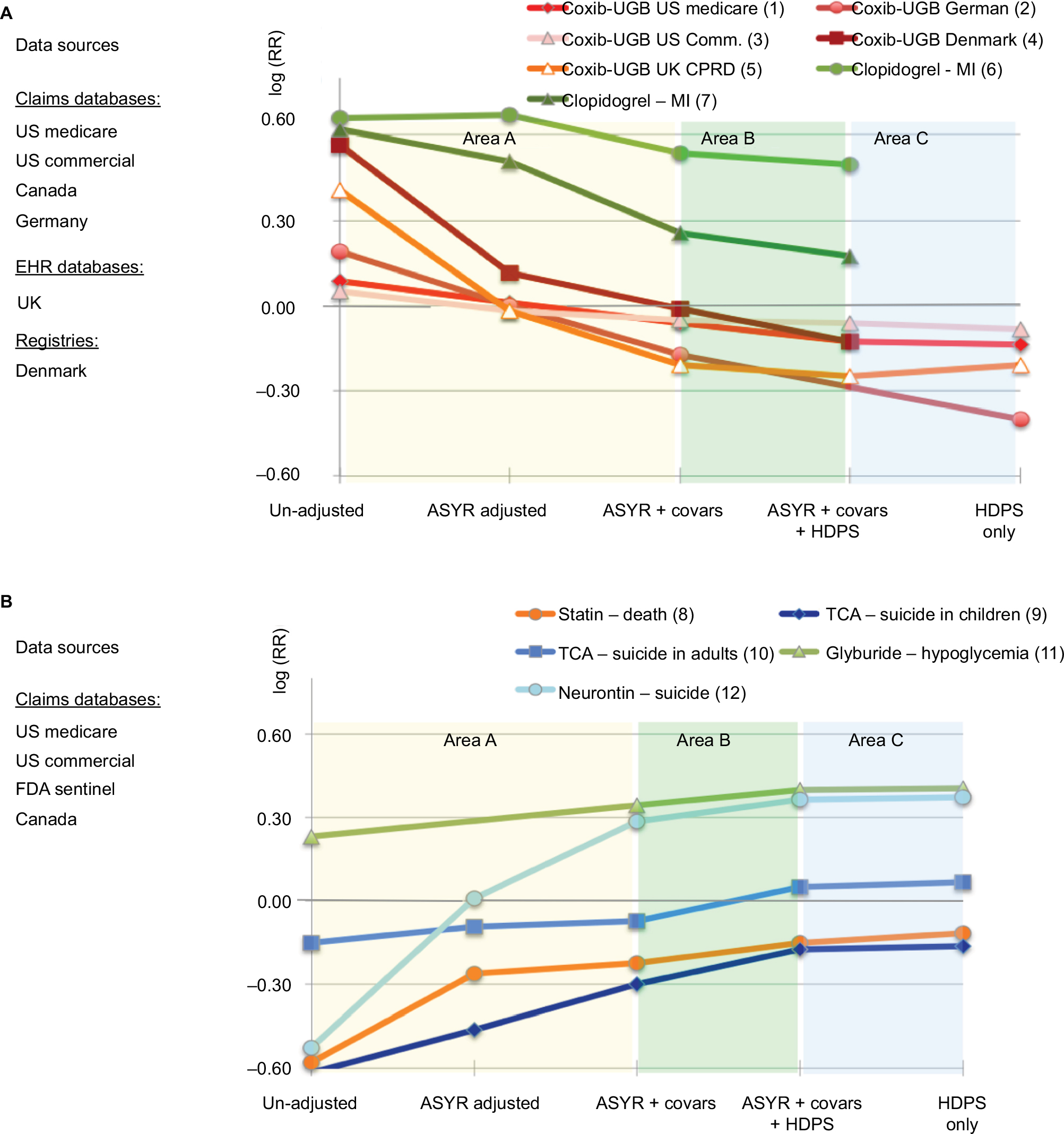Figure 6 Empirical performance of HDPS in selected health care database studies across a variety of settings. Notes: (A) Examples with declining trends in effect estimates (1),22 (2),54 (3),55 (4),56 (5),57 and (6,7).117 (B) Examples with increasing trends in effect estimates (8),22 (9),118 (10),119 (11),59 and (12).120 The number of covariates adjusted increases from left to right, and the log effect estimate is plotted on the y-axis centered around a null effect (log[RR] =0). Each colored graph represents the change in effect estimate for a specific study as the number of adjusted covariates (covars) increases. Abbreviations: ASYR, age, sex, year, race; covars, investigator-specified covariates; HDPS, high-dimensional propensity score; EHR, electronic health records; Coxib, cyclooxygenose-2 selective inhibitors; CPRD, Chemical Practise Research Datalink; MI myocardial infarction; FDA, US Food and Drug Administration; TCA, tricyclic antidepressants.

Several consistent observations can be made.

1. In Area A, while moving from an unadjusted estimate (at the very left) to an age, sex, year, race-adjusted estimate, and finally a model adjusted for all investigator-identified confounders, the changes in effect estimates follow a monotonically increasing or decreasing trend with increasing covariate adjustment. While this is not proof, it is strongly suggestive of increasing improvement in confounding adjustment. Note further that some of the lines cross the null, refuting concerns that we are simply observing a bias toward the null.
2. In Area B, the HDPS algorithm is added to the investigator-specified fully adjusted model. In all example studies, the point estimate is changing further in the monotonically increasing/decreasing trend. This is strongly suggestive of further confounding adjustment of the effect estimates applying the same logic as earlier.
3. In Area C, the HDPS algorithm is applied alone without the investigator-specified confounding adjustment. HDPS includes patient attributes such as age, sex, and race by default (Figure 5). It is noteworthy that applying the HDPS algorithm alone produced the same effect estimate as the investigator-specified adjustment plus the HDPS algorithm. This strongly suggests that even without the investigator-specifying covariates for adjustment, the algorithm alone optimizes confounding adjustment. In fact, it seems that in these examples, the algorithm performed slightly better than the investigator-derived estimates, as the monotonic trend in change of effect estimates continues from Area A to Area C.

Selected applications with structured health care data: medical product effectiveness

Five effectiveness studies were published on the lower gastrointestinal (GI) toxicity of cox-2-selective inhibition (coxibs) compared with nonselective non-steroidal anti inflammatory drugs (NSAIDs), all of which used HDPS. RCTs point to a relative risk reduction of between 10 and 25%.^52,53 Confounding arises because coxibs were heavily marketed for their GI-protective effects as compared to nonselective NSAIDs leading to their preferred use in patients of high risk for GI toxicity including upper gastric bleed (UGB). Some subtler GI risk factors are difficult to observe in many data sources, which raises concerns of unobserved confounding and makes this a useful testing scenario for HDPS. These studies used various data sources within and outside the USA. Our examples focus on point estimates.

• Garbe et al⁵⁴ worked with German claims data. They found estimates with increasing adjustment from 1.21 (unadjusted), 1.00 (plus age, sex, year), and 0.84 (plus investigator-identified). An HDPS-only model yielded 0.67, the most plausible estimate.
• Le et al⁵⁵ worked with US commercial claims data. They found estimates with increasing adjustment from 1.05 (unadjusted), 0.98 (plus age, sex), 0.95 (plus investigator-identified), and 0.94 (plus HDPS). The HDPS-only model produced 0.92, the most plausible estimate among those computed. However, the observed effect is still removed from the expected effect size observed in RCTs suggesting that the data may not have been sufficiently rich to minimize confounding.
• Schneeweiss et al²² used US Medicare claims data. They found estimates with increasing adjustment from 1.09 (unadjusted), 1.01 (plus age, sex, year, race), 0.94 (plus investigator-identified), and 0.88 (plus HDPS). An HDPS-only model yielded 0.87, similar to the combined clinical and HDPS estimate.
• Hallas and Pottegard worked with Danish registry data.⁵⁶ They found estimates with increasing adjustment from 1.76 (unadjusted), 1.12 (plus age, sex), 0.99 (plus investigator-identified), and 0.88 (plus HDPS). The HDPS-only model yielded 0.96. This study did not adjust for health care utilization markers such as the numbers of visits, which could have improved the estimation.
• Toh et al⁵⁷ used UK electronic health records from primary care physicians. They found estimates with increasing adjustment from 1.50 (unadjusted), 0.98 (plus age, sex, year), 0.81 (plus investigator-identified), and 0.78 (plus HDPS). An HDPS-only model resulted in 0.81, similar to the investigator-identified estimate. Interestingly, the investigator also included a model that included age, sex, year, and health services utilization (number of visits and number of drugs), which on its own changed the RR to 0.84 without including any investigator-identified covariates, demonstrating the importance of adjusting markers of health service utilization intensity.

These studies have in common that HDPS – in all situations and across different data sources – either improved the effect estimation by further extending the observed trend in estimate change or at least is on par with the investigator-specified adjustment model (Figure 6A). This illustrates the versatility of HDPS, independent of the data source or coding system.⁵⁸ These studies further underscore the value of routinely combining HDPS not only with obvious patient attributes (age, sex, race, and so on) but also markers of health services’ utilization intensity as a general marker of disease severity but also a proxy for medical surveillance and data completeness.

The Sentinel Program of the US food and Drug Administration routinely uses HDPS adjustment in its preprogrammed PS analysis ARIA module.⁵⁹ In a recent validation of this program, Sentinel Investigators attempted to reproduce the 52% risk increase (RR =1.52; 1.21–1.92) in hypoglycemic events among users of the oral antidiabetic drugs glyburide versus glipizide as observed in randomized trials.⁶⁰ They observed a 26% risk increase in an unadjusted analysis (1.16–1.38). Adjustment for investigator-specified covariates increased the relative risk to 1.41 (1.27–1.56), which came slightly closer to the RCT finding when HDPS was added (1.49; 1.34–1.65). The same finding was reached when HDPS was used alone as an automated procedure (1.50; 1.36–1.66). Zhou et al⁵⁹ also report that HDPS identified pregnancy and gestational diabetes as important treatment predictors and potential confounders. These covariates were not specified by a highly experienced team of investigators, highlighting the value of data-adaptive approaches to optimize confounding adjustment without omitting empirically identifiable confounders. Such unintentional omissions are likely not infrequent and may be even more prevalent among less-experienced research teams.

Selected applications with structured health care data: health services research

Enders et al⁶¹ investigated the quality of care in outpatient versus in-hospital percutaneous coronary interventions (PCI) regarding the risk of death using German commercial claims data. Confounding arose in this study, as healthier patients would be selected for outpatient PCI and higher risk patients would receive PCI in a hospital. An investigator-specified PS model including 39 covariates showed a 50% lower rate of death among patients undergoing outpatient PCI. The HDPS algorithm limited to 1000 covariates qualitatively changed the effect to a 20% increase in the risk of death when receiving PCI in an outpatient setting. This is an impressive illustration of massive residual confounding and HDPS’s ability to overcome it.

Using US Medicare claims data, Polinski et al⁶² investigated whether the coverage gap in Medicare Part D medication insurance plans would lead to adverse health effects in elderly patients. After patients had spent a certain amount on prescription drugs they reached the coverage gap, during which they were responsible for 100% of payment. Confounding arose in this study, as patients with poor health or low economic status were eligible for insurance subsidies and experienced no or a much reduced coverage gap. The same patients may also be a higher risk for poor health outcomes. Polinski contrasted confounding adjustment via 34 investigator-selected variables in a PS model versus an HDPS algorithm limited to 400 covariates. The effect of the coverage gap on the occurrence of heart failure hospitalization changed from a spurious 24% reduction in an unadjusted analysis to a null effect after adjustment. Both the investigator-specified and the automated HDPS adjustment provided similar results.

Selected applications with unstructured health care data

Using free text information for improved confounding control is promising in principle, because it supplements claims type information with more subtle considerations of disease and treatment that are not captured in highly structured data fields. Today, the analysis of free text information involves natural language processing (NLP) to characterize medical constructs. NLP requires the establishment of a gold standard, often via medical records’ review by medical experts, against which machine-learning algorithms can develop prediction rules. Such supervised learning is expensive and time consuming and therefore not meaningfully scalable for confounding adjustment.

HDPS is well suited to automate covariate adjustment of free text information. Rassen et al⁶³ separated free text information into individual word stems and clustered them into phrases of 1, 2, or 3 consecutive word stems (N-grams). The N-grams served as binary markers (N-gram present or not) that were considered by the HDPS algorithm. Out of thousands of N-grams, the top 500 were selected by HDPS and used for covariate adjustment. An unadjusted effect estimate of the incidence of cardiovascular (CV) outcomes comparing high-intensity statin therapy vs low-intensity statin therapy in patients with hyperlipidemia showed a spurious doubling in risk (RR =2.19; 1.71–2.80), which was reduced to 1.21 by adjusting for investigator-specified variables, and was further reduced to 0.96 with the automated N-gram approach (Figure 7).⁶³

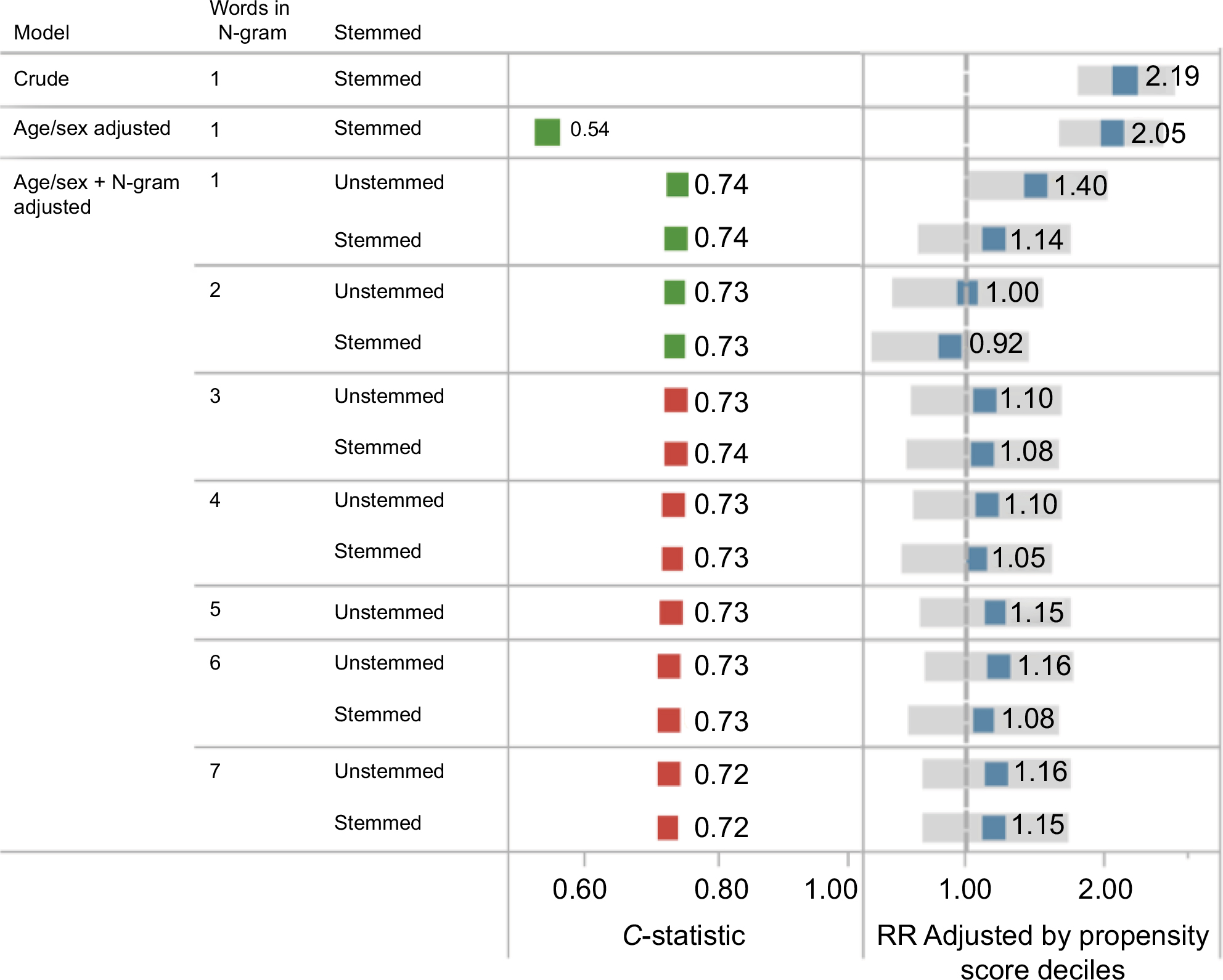Figure 7 Automated covariate adjustment from free text medical notes using N-gram analysis and HDPS. Notes: N-grams are contiguous sequence of one-, two-, or three-word stems from a medical note text; plotted are relative estimates (blue) with 95% confidence intervals (gray bars). In this example, a null effect was expected (RR =1, dashed vertical line). Data from Rassen et al.63 Abbreviations: HDPS, high-dimensional propensity score; RR, relative risk.

This content-agnostic and therefore eminently scalable approach to adjusting for free-text information serves as a proof of concept to be followed by more in-depth investigations. NLP or mapping free text to established ontologies such as SNOMED and sentiment analysis become unnecessary intermediate steps with unclear benefits.

Selected applications with adjustment for time-varying confounding

A natural application of HDPS is in the setting of time-varying exposures with time-varying confounding via marginal structural models.⁶⁴ Since propensity score estimation and weighting, eg, matching weighting and inverse probability of treatment weighting,⁴⁷ are central to studies of time-varying exposures, conventional PS estimation is simply replaced by HDPS in hopes of better predicting treatment choice.

A cohort study of adults with type-2 diabetes mellitus (T2DM) was conducted to evaluate the impact of progressively more aggressive glucose-lowering strategies.⁶⁵ To account for time-dependent confounding and informative selection bias, a marginal structural model⁶⁶ was fitted using PS weighting for the purpose of contrasting cumulative risks under four treatment escalation strategies at Hb_A1c levels 7, 7.5, 8, or 8.5%.⁶⁵

While the HDPS algorithm fit into the marginal structural model design, it did not show substantial improvement in the specific study setup. This is because the variable space allowed for HDPS was limited to the investigator-identified covariates, which did not allow HDPS to automatically identify relevant covariates that an investigator might not have considered.⁶⁵

The opportunities of data-adaptive methods are summarized in Box 1.

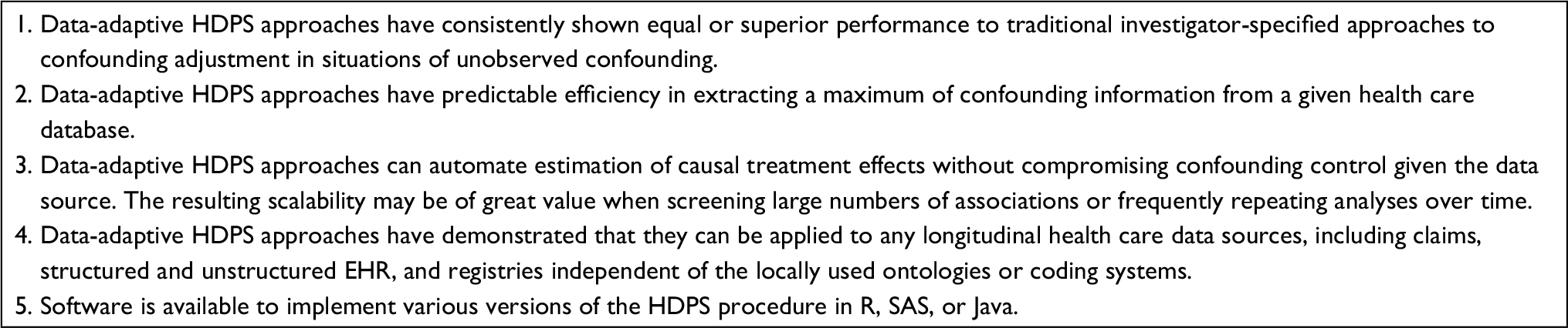Box 1 Opportunities of data-adaptive HDPS approaches for causal treatment-effect estimation using health care databases Abbreviations:HDPS, high-dimensional propensity score; EHR electronic health records.

Simulation studies of HDPS performance in health care database analyses

Several simulation studies sought to examine HDPS’ ability to better adjust for unobserved confounding via proxy-adjustment. Since fully synthetic simulation studies fail to mimic the complexity of highly interrelated longitudinal health care databases, which is the primary motivator for successful proxy adjustment, plasmode simulation was developed.⁶⁷ Based on an empirical health care dataset, a patient cohort with the exposures of interest is identified and an outcome function with known effect size and randomness is introduced to the cohort.⁶⁷ This approach preserves the complexity of the data structure and information content while inserting a known causal effect.

Rassen et al³⁹ studied how well HDPS performs when study sizes are smaller and fewer or no outcomes have been observed, which may apply to settings of prospective studies of newly marketed medical products. This showed that the effect estimation using HDPS-decile adjustment was becoming increasingly volatile when very few patients were exposed (see section on sparse data). In such situations the simulation study suggested it might be more valid on average to only consider the covariate-outcome association for covariate prioritization.

Wyss et al,⁶⁸ in a most comprehensive plasmode simulation based on three empirical cohort studies, focused on fully automated confounding control and confirmed the superior performance of HDPS in a series of settings. Across three settings times six simulation scenarios, depending on the frequency of exposure and outcome, HDPS with 100 bias-prioritized covariates^22,38 showed an average 90–95% bias reduction without any investigator-specified covariates and never less than 70% bias reduction.⁶⁸

Franklin et al⁴² compared the performance of HDPS in a plasmode simulation to that in an outcome model using regularized regression including Lasso and ridge regression, adjusting for a prioritized pool of 500 candidate covariates. Both Lasso and ridge regression outcome models underperformed compared with HDPS. However, when Lasso was used to prioritize covariates regarding their association with the outcome, which were then entered into the PS model, this resulted in an improved performance following the principles of confounder selection.^34,35,69

Guertin et al⁷⁰ published an empirical study but included a sensitivity analysis simulating unobserved confounding. In a study comparing low-intensity versus high-intensity lipid-lowering therapy with statins, they were concerned that sicker patients with more advanced arteriosclerosis or higher serum lipid levels were more likely to initiate high-intensity treatment. Residual confounding can be caused by unobserved risk factors such as family history, actual lipid levels, and unobserved diagnostic information after omitting outpatient claims. They compared balance in covariates in two Quebec health care claims databases, one with full information and one with strongly restricted data dimensions. They found that despite artificially reducing the amount of covariate information by 86%, the HDPS algorithm would still correctly identify and balance important confounders not directly observable.

Machine-learning extensions to optimize automated covariate selection

Within the framework of HDPS, there have been several machine-learning extensions that can help further optimize and automate the critical covariate prioritization.

Principles of covariate selection in PS models

Rosenbaum and Rubin⁷¹ and Rubin⁷² recommend that covariates for a PS model should be selected based on whether the variables balance confounding factors between exposure groups. This assumes that investigators know and measure all true confounders, an assumption that is unrealistic in most secondary analyses of health care databases. The FDA Sentinel analysis by Zhou et al⁵⁹ is such an example of an important confounder that was not identified by the investigator team yet was measurable in the data. It has been established that all independent risk factors for the study outcome need to be adjusted even if they are seemingly not or only weakly associated with the exposure.^34,35,69 An automated algorithm thus should select covariates based on empirically observed outcome associations as long as variable selection is not influenced by the magnitude of the treatment effect estimate.^22,34

Optimized automated covariate prioritization

Because of the importance of the confounder–outcome relationship for covariate selection, it is not surprising that machine-learning approaches to optimize only the treatment model, including regularized regression, classification and regression trees (CART), multivariate adaptive regression spline (MARS), and random forest, while being mechanically useful, did not improve causal inference.^73–76 In fact, intensive modeling of only the exposure without considering the relationship with the study outcome may increase the chance of including features that act as instrumental variables and exacerbate residual confounding bias.^36,77 Although regularized outcome regression such as Lasso can model the outcome association of many covariates simultaneously even if outcomes are sparse, they are inadequate in its confounding adjustment when studying causal treatment effects, as they shrink or eliminate regression coefficients, reducing the amount of information on the confounder–outcome association, ultimately leading to biased effect estimates.⁴²

Therefore, the focus logically shifted toward empirically identifying potential predictors of the study endpoint but, instead of adjusting them in an overfitted outcome model, prioritizing them in the PS model.⁷⁸ A reanalysis of five cohort studies evaluated a range of machine-learning algorithms to empirically identify and prioritize outcome predictors, including Lasso, ridge regression, logistic regression, Bayesian logistic regression, random forests, elastic net, and principal component analysis. It showed that a Lasso-based selection of outcome predictor into the PS model may be a flexible and robust hybrid strategy, which in claims data on average performs just slightly better than the originally proposed easy-to-understand Bross formula.⁷⁸ A slight advantage of covariate prioritization that is informed by outcome regression as hybrid strategy was confirmed in further simulation studies.^42,79,80 The full potential of such informally “doubly robust” hybrid strategies may be realized when information-rich databases are used that can predict outcomes better than claims data.

Automatically optimized number of covariates

Several studies had suggested that there may be an optimum number of empirically identified and prioritized covariates that should be included in the PS for causal analyses.^39,81 It was the hope that with increasing covariate adjustment in prioritized sequence, the exposure–outcome effect estimate would stabilize and approximate the value of the best adjusted effect estimate given the information inherent in a database. However, this does not seem to hold when exposure is infrequent and outcomes rare.⁸¹ Other strategies need to be applied to identify the optimum confounder adjustment.

When the optimum number of covariates for adjustment is not known, analysts can run several HDPS models with various numbers of prioritized covariates. Super Learner, an ensemble method for prediction modeling,⁸² can obtain optimal predictions. These predictions will be similar to those from the regression with the optimum number of important variables, in terms of minimizing a cross-validated loss of function for predicting treatment assignment. Extensive plasmode simulations based on three empirical cohort studies showed that the combination of Super Learner with HDPS as a fully automated strategy avoided inadvertent overfitting and outperformed in a range of scenarios.⁶⁸

After covariate prioritization, one can combine Super Learner with the HDPS to simplify propensity score estimation in high-dimensional covariate settings.

Collaborative targeted maximum likelihood estimation (CTMLE), pioneered by van der Laan, is a similar approach to automating and optimizing causal analyses with nonrandomized data. It includes an exposure model (PS model) and an outcome model, both automatically optimized via Super Learner, combined with a doubly robust effect estimation that is focused (targeted) on the effect of interest, thus optimizing statistical efficiency. CTMLE is a generalized framework for causal inference, while HDPS is optimized for health care databases with the majority of variables being binary or categorical. Because HDPS is not dependent on estimating an outcome model for covariate adjusted-effect estimation but only for covariate prioritization, it is more robust in settings of rare outcomes and many covariates.^68,83

Sparse data: treatment effects of newly marketed products and highly targeted treatments

Even with the largest data sources, there are situations in which exposures are infrequent. Examples are highly targeted treatments often preselected by specific biomarkers or treatments for orphan diseases and the study of newly approved medications when few patients have been exposed shortly after they reach the market.⁸⁴ These are treatments and conditions of high relevance and challenge any method of treatment-effect estimation including HDPS.

Being aware of this challenge, an empirically based simulation study showed that, given ~<25 exposed patients who have an outcome event, the estimation of effect using HDPS decile adjustment was volatile.³⁹ The work by Patorno et al⁸¹ identified equally strong variability of effect estimates after PS matching with increasing HDPS covariate counts. Adjusting for a continuous PS variable or PS deciles seemed to perform better than matching. In the setting of very few outcomes, including or excluding single events due to successful or failed matching can substantially change the magnitude of effects. A simulation study confirmed that in situations of very few outcomes, PS adjustment or PS weighting may perform better than matching.⁸⁵ More analyses clarified that specifically when the exposure is infrequent, HDPS may lead to overfitting more residual bias but not when the exposure is frequent and only the outcome is rare.⁶⁸ Fine stratification by PS is another robust approach for PS analyses when exposure is infrequent.⁴⁵ While this issue is not specific to HDPS, knowing that stratified or weighting approaches may be more robust in such settings will guide automated strategies. The situation of infrequent exposure and rare outcomes may favor disease risk score (DRS) approaches and the use of HDDRS with covariate prioritization incorporating risk prediction information from historical data.^50,86

“Over-adjustment” and the importance of causal study designs

It is a misconception that data-adaptive algorithms that adjust hundreds of covariates will lead to over-adjustment. An over-adjustment stemming from the adjustment of causal intermediates, reverse causation, or immortal person-time are general study design concerns that are addressable with principled study designs to support causal inference and, if present, can cause bias often larger in magnitude than confounding.^87,88 A common concern, adjusting for too many pre-exposure covariates, will lead to collinearity and statistical inefficiency in the estimation but does not constitute over-adjustment and effect estimates remain consistent.⁷¹

There are two complex covariate structures worth mentioning, as they have been seen as complicating automated covariate adjustment.⁸⁸ M-bias occurs from conditioning on an apparent confounder (C), which is actually a collider in the language of directed acyclic graphs.⁸⁹ The study of the risk of antidepressants in relation to lung cancer assumed that U1 is a depression status (affecting antidepressant use but not lung cancer) and U2 is a smoking history (affecting lung cancer but not antidepressant use). By conditioning on cardiovascular disease (C), an association is induced between antidepressants and lung cancer via the M-shaped pathway via depression, cardiovascular disease, and smoking.⁸⁹ Simulation studies have shown that even in extreme scenarios, any resulting bias was minor.⁹⁰ In the majority of empirical settings, the reduction in bias from adjusting for the confounding will outweigh any increase in bias due to conditioning on a collider.⁹¹

Z-bias refers to the bias caused by adjusting for an instrumental variable in studies that are subject to meaningful unmeasured confounding.^36,92 An instrument is a variable that is associated only with the exposure and not with outcome other than through the exposure.^93,94 In a study of the effect of statins versus glaucoma drugs on the incidence of myocardial infarction, a variable such as prior glaucoma diagnosis will be strongly predictive of whether a patient receives a glaucoma drug but will have little effect on the outcome.

A simulation study found that Z-bias, while measureable, was of substantial magnitude only in cases of very strong unmeasured confounding, and even in these cases, the strongest Z-bias that could be observed was <5% of the total study bias. When in doubt about whether a covariate is a confounder or an instrument, adjusting for the covariate will generally reduce net bias.³⁶ More complex automated methodologies are available, but their added value in high-dimensional data settings has come into question.^95,96

Potential misconceptions about data-adaptive methods are summarized in Box 2.

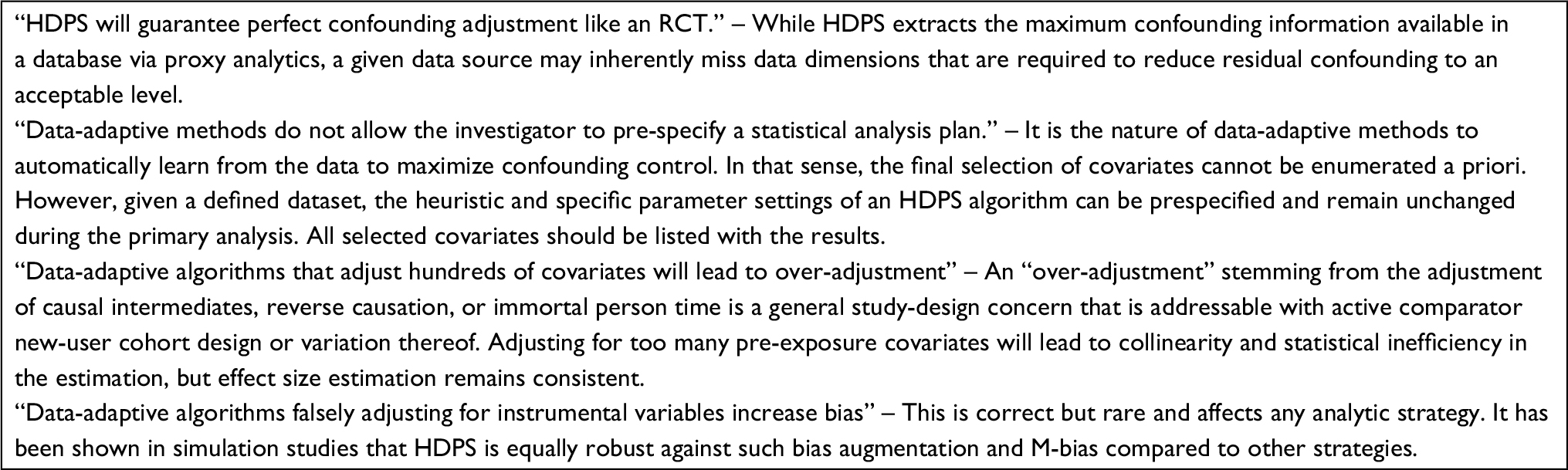Box 2 Misconceptions about data-adaptive methods for confounding control Abbreviations:HDPS, high-dimensional propensity score; RCTs, randomized controlled trials.

Pathway to automating causal treatment effect estimation in health care databases

The most frequent application of analytics in a learning health care system is that of comparing the effectiveness of two interventions, two clinical strategies, or two medical products.⁹⁷ For most applications, it would be a valuable simplification if a user would just specify the exposures, outcome(s), and target population and let an automated data-adaptive algorithm such as HDPS process the causal analytics. If one is willing to make some constraining assumptions, the process of designing and analyzing database studies for causal treatment effect becomes a linear process with defined choices that is increasingly automatable (Figure 8).²⁸ For example, for a range of applications, one may generally prefer a new-user cohort study design in database studies without addition of data collection, dismissing sampling strategy (case–control, case–cohort); one may focus on baseline covariates and not consider treatment changes and time-varying confounding; one may always want to compute ratio as well as difference effect measures including 95% confidence intervals and implement a fixed follow-up (risk model) as well as an as-treated follow-up (rate model) analysis.

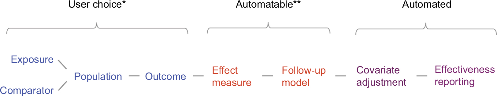Figure 8 Toward automating causal treatment effect estimation. Notes: *These items are highly structured, and modern Real World Data software facilitates this critical interface between intended research questions and study implementation. **There is a limited number of context-specific choices. Reasonable defaults can be provided, and RWD software will allow users to override.

The use of HDPS is now an accepted tool among database researchers.²³ Some database studies even show results only after HDPS adjustment, a logical consequence of the consistent performance advantages of HDPS in database studies.^98–100 The next rational step is to use data-adaptive approaches as a fully automated confounding adjustment approach rather than as a secondary analysis confirming or improving traditional approaches.

The scalability of automated covariate adjustment has been demonstrated: independent of coding system and regional differences in data structures, the HDPS algorithm performed as well or better than investigator-defined methods. With new advances in hybrid doubly robust approaches, super-learner enhancements and fine stratification of HDPS perform well in tricky situations of few exposed patients and rare outcomes. By embedding such adjustments in standard causal study designs, including new-user active comparator cohorts and marginal structural models, other biases – often more extreme than confounding – can be reduced as well.²⁸ Automation, however, would need to be accompanied by quality metrics of the likely success of confounding control, something that requires further research in order to become sufficiently confidence building.^101,102

Multidatabase studies

Automated and optimized confounding adjustment approaches play an important role in multidatabase systems that are queried in rapid cycles to monitor the effectiveness or safety of medical products and interventions. Given variations among databases in terms of information content, terminology, and coding practices, a strategy that allows maximizing confounding control in a given data source independent of the coding system will provide the most valid results rapidly. Alternative strategies, such as data standardization and distributed regression analyses, work with the minimum common denominator of information but fail to embrace the reality of substantial variations in information content between data sources.¹⁰³ In extreme situations, more confounding control in some data sources than others, say those with claims data linked to free text medical notes versus those with claims only, may lead to point estimates with reduced bias. Such heterogeneity must bring up questions as to whether it makes sense to use all databases in a network for a given analysis or rather only those with richer information.

Considering these advantages, large regulatory drug safety monitoring programs have adopted HDPS. FDA’s drug safety surveillance program, the Sentinel Program, has integrated HDPS into its routine propensity score matching program as a standard analysis for data source-optimized confounding adjustment.^104,105 The PS modular program was independently compared against investigator-specified analyses and RCT findings.^59,106 The Canadian counterpart, the CNODES program, uses HDPS as well.^107,108

In multidatabase studies, we frequently find situations of several very large databases and multiple fairly small centers, yielding small numbers of exposed patients particularly when studying newly marketed medications. An HDPS model with >100 covariates may not fit in such settings,⁵⁹ and the machine-learning extensions, particularly Super Learner, would be applied. In contrast, not including small sites did not change the findings in the Sentinel Program, since they did not contribute much information in the first place.⁵⁹

Large-scale screening of drug repurposing

Medications are marketed for specific indications defined by a condition treated and outcome(s) improved. In routine care, medications are not infrequently used outside of narrow indications to treat conditions of similar pathophysiology and/or different outcomes. Repurposing already marketed drugs is appealing because they have already passed substantial testing in humans and are considered sufficiently safe for use, and therefore, the uncertainty of having a secondary indication approved is much reduced. Large health care databases have been considered many times to discover unexpected beneficial drug effects.

Rather than scanning the entire potential drug–outcome space with all its combinations, more promising approaches rely on network proximity quantifying the interplay between disease genes, proteins, and drug targets on the human interactome to reveal hundreds of new potential drug–outcome associations.^109,110 Health care database analyses can then validate or refute high-potential drug–outcome associations,¹¹¹ but even reducing many thousands of associations to only a few hundred will require a scalable approach to confounding adjustment as it is impractical to have investigator-defined covariate selection for each study.¹¹² Data-adaptive methods for optimized confounding adjustment will have an important role in ongoing repurposing programs.

Transparency, reporting, and diagnostics

By definition, data-adaptive strategies intended to control confounding cannot predefine the exact covariates or even the number of covariates that will go into the final analysis. However, what can be prespecified and incorporated into study registration databases is the specific analytic strategy and parameter settings of the automated approach for covariate identification, prioritization, and type of causal analysis. After the analysis has been completed, the algorithm can produce the exact list of covariates that were actually included in the PS model.¹¹³ In addition, graphs that show the relationship between the sequential addition of prioritized covariates and the corresponding changes in the treatment effect estimate are of great diagnostic value.^39,54,81 We generally need more robust diagnostics on the completeness of confounding control. While complete knowledge on confounding may always be elusive, developments in balance metrics of observed characteristics and systems that test balance in patient subgroups that have confounders defined that are unobservable in the main study are promising.^{101,102,114,115}

Conclusion

Data-adaptive approaches to automated and optimized covariate adjustment for estimating causal treatment effects in health care databases, such as the HDPS algorithm, are remarkably effective and often superior in terms of bias reduction across a range of research questions and versatile in a variety of data sources and coding systems. The properties of HDPS are well understood based on empirical studies and statistical simulation experiments. Building on the principles of HDPS, we are approaching fully automated covariate adjustment procedures scalable across health care databases that reduce bias to the degree possible by a given data source. This has important implications for the evaluation of causal treatment effects in one-off analyses, for safety-signal generation, for large-scale screening for the effectiveness of secondary indication or repurposing, or multi database networks.

Acknowledgments

The author is grateful for numerous valuable discussions with his colleagues Jeremy A Rassen, Robert J Glynn, Jessica M Franklin, and Richie Wyss as well as most helpful insights from Mark van der Laan and Alec Walker. This work is the fruit of years of close collaboration in the Methods Incubator Group in the Division of Pharmacoepidemiology, for which the author is most thankful. This work was funded in part by the Patient-centered Outcomes Research Institute. SS was also funded by the National Institutes of Health and the US Food and Drug Administration.

Disclosure

SS is a consultant to WHISCON, LLC, and to Aetion, Inc., a software manufacturer of which he also owns equity. He is a principal investigator of research grants to the Brigham and Women’s Hospital from Bayer, Genentech, and Boehringer Ingelheim unrelated to the topic of this article. The author reports no other conflicts of interest in this work.

References

1.		Arana A, Rivero E, TCG E. What do we show and who does so? An analysis of the abstracts presented at the 19th ICPE. Pharmacoepidemiol Drug Saf. 2004;30:S330–S331.
2.		Suissa S, Garbe E. Primer: administrative health databases in observational studies of drug effects – advantages and disadvantages. Nat Clin Pract Rheumatol. 2007;3(12):725–732.
3.		Schneeweiss S, Avorn J. A review of uses of health care utilization databases for epidemiologic research on therapeutics. J Clin Epidemiol. 2005;58(4):323–337.
4.		Ray WA. Evaluating medication effects outside of clinical trials: new-user designs. Am J Epidemiol. 2003;158(9):915–920.
5.		Johnson ES, Bartman BA, Briesacher BA, et al. The incident user design in comparative effectiveness research. Pharmacoepidemiol Drug Saf. 2013;22(1):1–6.
6.		Seeger JD, Walker AM, Williams PL, Saperia GM, Sacks FM. A propensity score-matched cohort study of the effect of statins, mainly fluvastatin, on the occurrence of acute myocardial infarction. Am J Cardiol. 2003;92(12):1447–1451.
7.		Graham DJ, Reichman ME, Wernecke M, et al. Cardiovascular, bleeding, and mortality risks in elderly Medicare patients treated with dabigatran or warfarin for nonvalvular atrial fibrillation. Circulation. 2015;131(2):157–164.
8.		Schneeweiss S, Seeger JD, Landon J, Walker AM. Aprotinin during coronary-artery bypass grafting and risk of death. N Engl J Med. 2008;358(8):771–783.
9.		Kim SC, Solomon DH, Rogers JR, et al. Cardiovascular safety of tocilizumab versus tumor necrosis factor inhibitors in patients with rheumatoid arthritis – a Multi-database Cohort Study. Arthritis Rheum. 2016;69(6):1154–1164.
10.		Ray WA, Chung CP, Murray KT, Hall K, Stein CM. Atypical antipsychotic drugs and the risk of sudden cardiac death. N Engl J Med. 2009;360(3):225–235.
11.		Wang PS, Schneeweiss S, Avorn J, et al. Risk of death in elderly users of conventional vs. atypical antipsychotic medications. N Engl J Med. 2005;353(22):2335–2341.
12.		Ebrahim S, Sohani ZN, Montoya L, et al. Reanalyses of randomized clinical trial data. JAMA. 2014;312(10):1024–1032.
13.		Poynter JN, Gruber SB, Higgins PD, et al. Statins and the risk of colorectal cancer. N Engl J Med. 2005;352(21):2184–2192.
14.		Go AS, Lee WY, Yang J, Lo JC, Gurwitz JH. Statin therapy and risks for death and hospitalization in chronic heart failure. JAMA. 2006;296(17):2105–2111.
15.		Chan KA, Andrade SE, Boles M, et al. Inhibitors of hydroxymethylglutaryl-coenzyme A reductase and risk of fracture among older women. Lancet. 2000;355(9222):2185–2188.
16.		Franklin JM, Schneeweiss S. When and how can real world data analyses substitute for randomized controlled trials? Clin Pharmacol Ther. 2017;102(6):924–933.
17.		Walker AM. Confounding by indication. Epidemiology. 1996;7(4):335–336.
18.		Petri H, Urquhart J. Channeling bias in the interpretation of drug effects. Stat Med. 1991;10(4):577–581.
19.		Maclure M, Schneeweiss S. Causation of bias: the episcope. Epidemiology. 2001;12(1):114–122.
20.		Glynn RJ, Knight EL, Levin R, Avorn J. Paradoxical relations of drug treatment with mortality in older persons. Epidemiology. 2001;12(6):682–689.
21.		Setoguchi S, Warner Stevenson L, Stewart GC, et al. Influence of healthy candidate bias in assessing clinical effectiveness for implantable cardioverter-defibrillators: cohort study of older patients with heart failure. BMJ. 2014;348:g2866.
22.		Schneeweiss S, Rassen JA, Glynn RJ, Avorn J, Mogun H, Brookhart MA. High-dimensional propensity score adjustment in studies of treatment effects using health care claims data. Epidemiology. 2009;20(4):512–522.
23.		Cadarette SM, Ban JK, Consiglio GP, et al. Diffusion of innovations model helps interpret the comparative uptake of two methodological innovations: co-authorship network analysis and recommendations for the integration of novel methods in practice. J Clin Epidemiol. 2017;84:150–160.
24.		Schneeweiss S. Understanding secondary databases: a commentary on “Sources of bias for health state characteristics in secondary databases”. J Clin Epidemiol. 2007;60(7):648–650.
25.		Gini R, Schuemie M, Brown J, et al. Data extraction and management in networks of observational health care databases for scientific research: a comparison of EU-ADR, OMOP, mini-sentinel and MATRICE strategies. EGEMS (Wash DC). 2016;4(1):1189.
26.		Curtis LH, Weiner MG, Boudreau DM, et al. Design considerations, architecture, and use of the mini-sentinel distributed data system. Pharmacoepidemiol Drug Saf. 2012;21(suppl 1):23–31.
27.		Matcho A, Ryan P, Fife D, Reich C. Fidelity assessment of a clinical practice research datalink conversion to the OMOP common data model. Drug Saf. 2014;37(11):945–959.
28.		Schneeweiss S. A basic study design for expedited safety signal evaluation based on electronic healthcare data. Pharmacoepidemiol Drug Saf. 2010;19(8):858–868.
29.		Wooldridge JM. Econometric Analysis of Cross Section and Panel Data. Cambridge, MA: MIT Press; 2002.
30.		Gelman A, Carlin J, Stern H, Rubin D. Bayesian Data Analysis. New York: Chapman Hall; 1995.
31.		Suissa S, Blais L, Ernst P. Patterns of increasing beta-agonist use and the risk of fatal or near-fatal asthma. Eur Respir J. 1994;7(9):1602–1609.
32.		Rassen JA, Schneeweiss S. Using high-dimensional propensity scores to automate confounding control in a distributed medical product safety surveillance system. Pharmacoepidemiol Drug Saf. 2012;21(suppl 1):41–49.
33.		Schuster T, Pang M, Platt RW. On the role of marginal confounder prevalence – implications for the high-dimensional propensity score algorithm. Pharmacoepidemiol Drug Saf. 2015;24(9):1004–1007.
34.		Robins JM, Mark SD, Whitney KN. Estimating exposure effects by modelling the expectation of exposure conditional on confounders. Biometrics. 1992;48(2):479–495.
35.		Brookhart MA, Schneeweiss S, Rothman KJ, Glynn RJ, Avorn J, Stürmer T. Variable selection for propensity score models. Am J Epidemiol. 2006;163(12):1149–1156.
36.		Myers JA, Rassen JA, Gagne JJ, et al. Effects of adjusting for instrumental variables on bias and precision of effect estimates. Am J Epidemiol. 2011;174(11):1213–1222.
37.		Greenland S. Invited commentary: variable selection versus shrinkage in the control of multiple confounders. Am J Epidemiol. 2008;167(5):523–529; discussion 530–531.
38.		Bross ID. Spurious effects from an extraneous variable. J Chronic Dis. 1966;19(6):637–647.
39.		Rassen JA, Glynn RJ, Brookhart MA, Schneeweiss S. Covariate selection in high-dimensional propensity score analyses of treatment effects in small samples. Am J Epidemiol. 2011;173(12):1404–1413.
40.		Schneeweiss S, Seeger JD, Maclure M, Wang PS, Avorn J, Glynn RJ. Performance of comorbidity scores to control for confounding in epidemiologic studies using claims data. Am J Epidemiol. 2001;154(9):854–864.
41.		Peduzzi P, Concato J, Kemper E, Holford TR, Feinstein AR. A simulation study of the number of events per variable in logistic regression analysis. J Clin Epidemiol. 1996;49(12):1373–1379.
42.		Franklin JM, Eddings W, Glynn RJ, Schneeweiss S. Regularized regression versus the high-dimensional propensity score for confounding adjustment in secondary database analyses. Am J Epidemiol. 2015;182(7):651–659.
43.		Cepeda MS, Boston R, Farrar JT, Strom BL. Comparison of logistic regression versus propensity score when the number of events is low and there are multiple confounders. Am J Epidemiol. 2003;158(3):280–287.
44.		Sturmer T, Rothman KJ, Avorn J, Glynn RJ. Treatment effects in the presence of unmeasured confounding: dealing with observations in the tails of the propensity score distribution – a simulation study. Am J Epidemiol. 2010;172(7):843–854.
45.		Desai RJ, Rothman KJ, Bateman BT, Hernandez-Diaz S, Huybrechts KF. A propensity-score-based fine stratification approach for confounding adjustment when exposure is infrequent. Epidemiology. 2017;28(2):249–257.
46.		Hernán MA, Brumback B, Robins JM. Marginal structural models to estimate the causal effect of zidovudine on the survival of HIV-positive men. Epidemiology. 2000;11(5):561–570.
47.		Yoshida K, Hernandez-Diaz S, Solomon DH, et al. Matching weights to simultaneously compare three treatment groups: comparison to three-way matching. Epidemiology. 2017;28(3):387–395.
48.		Moore KL, Neugebauer R, van der Laan MJ, Tager IB. Causal inference in epidemiological studies with strong confounding. Stat Med. 2012;31(13):1380–1404.
49.		Arbogast PG, Ray WA. Use disease risk scores in pharmacoepidemiologic studies. Stat Methods Med Res. 2009;18(1):67–80.
50.		Kumamaru H, Schneeweiss S, Glynn RJ, Setoguchi S, Gagne JJ. Dimension reduction and shrinkage methods for high dimensional disease risk scores in historical data. Emerg Themes Epidemiol. 2016;13:5.
51.		Kumamaru H, Gagne JJ, Glynn RJ, Setoguchi S, Schneeweiss S. Comparison of high-dimensional confounder summary scores in comparative studies of newly marketed medications. J Clin Epidemiol. 2016;76:200–208.
52.		Bombardier C, Laine L, Reicin A, et al; VIGOR Study Group. Comparison of upper gastrointestinal toxicity of rofecoxib and naproxen in patients with rheumatoid arthritis. VIGOR Study Group. N Engl J Med. 2000;343(21):1520–1528.
53.		Silverstein FE, Faich G, Goldstein JL, et al. Gastrointestinal toxicity with celecoxib vs nonsteroidal anti-inflammatory drugs for osteoarthritis and rheumatoid arthritis: the CLASS study: a randomized controlled trial. Celecoxib Long-term Arthritis Safety study. JAMA. 2000;284(10):1247–1255.
54.		Garbe E, Kloss S, Suling M, Pigeot I, Schneeweiss S. High-dimensional versus conventional propensity scores in a comparative effectiveness study of coxibs and reduced upper gastrointestinal complications. Eur J Clin Pharmacol. 2013;69(3):549–557.
55.		Le HV, Poole C, Brookhart MA, et al. Effects of aggregation of drug and diagnostic codes on the performance of the high-dimensional propensity score algorithm: an empirical example. BMC Med Res Methodol. 2013;13:142.
56.		Hallas J, Pottegard A. Performance of the high-dimensional propensity score in a nordic healthcare model. Basic Clin Pharmacol Toxicol. 2017;120(3):312–317.
57.		Toh S, Garcia Rodriguez LA, Hernan MA. Confounding adjustment via a semi-automated high-dimensional propensity score algorithm: an application to electronic medical records. Pharmacoepidemiol Drug Saf. 2011;20(8):849–857.
58.		Lin KJ, Schneeweiss S. Considerations for the analysis of longitudinal electronic health records linked to claims data to study the effectiveness and safety of drugs. Clin Pharmacol Ther. 2016;100(2):147–159.
59.		Zhou M, Wang SV, Leonard CE, et al. Sentinel modular program for propensity score-matched cohort analyses: application to glyburide, glipizide, and serious hypoglycemia. Epidemiology. 2017;28(6):838–846.
60.		Gangji AS, Cukierman T, Gerstein HC, Goldsmith CH, Clase CM. A systematic review and meta-analysis of hypoglycemia and cardiovascular events: a comparison of glyburide with other secretagogues and with insulin. Diabetes Care. 2007;30(2):389–394.
61.		Enders D, Ohlmeier C, Garbe E. The potential of high-dimensional propensity scores in health services research: an exemplary study on the quality of care for elective percutaneous coronary interventions. Health Serv Res. 2018;53(1):197–213.
62.		Polinski JM, Schneeweiss S, Glynn RJ, Lii J, Rassen JA. Confronting “confounding by health system use” in Medicare part D: comparative effectiveness of propensity score approaches to confounding adjustment. Pharmacoepidemiol Drug Saf. 2012;21(suppl 2):90–98.
63.		Rassen JA, Wahl PM, Angelino E, Seltzer MI, Rosenman MD, Schneeweiss S. Automated use of electronic health record text data to improve validity in pharmacoepidemiology studies. Pharmacoepidemiol Drug Saf. 2013;22(S1):376.
64.		Murphy SA, van der Laan MJ, Robins JM; CPPRG. Marginal mean models for dynamic regimes. J Am Stat Assoc. 2001;96(456):1410–1423.
65.		Neugebauer R, Schmittdiel JA, Zhu Z, Rassen JA, Seeger JD, Schneeweiss S. High-dimensional propensity score algorithm in comparative effectiveness research with time-varying interventions. Stat Med. 2015;34(5):753–781.
66.		Robins JM, Hernan MA, Brumback B. Marginal structural models and causal inference in epidemiology. Epidemiology. 2000;11(5):550–560.
67.		Franklin JM, Schneeweiss S, Polinski JM, Rassen JA. Plasmode simulation for the evaluation of pharmacoepidemiologic methods in complex healthcare databases. Comput Stat Data Anal. 2014;72:219–226.
68.		Wyss R, Schneeweiss S, van der Laan M, Lendle SD, Ju C, Franklin JM. Using super learner prediction modeling to improve high-dimensional propensity score estimation. Epidemiology. 2018;29(1):96–106.
69.		Leacy FP, Stuart EA. On the joint use of propensity and prognostic scores in estimation of the average treatment effect on the treated: a simulation study. Stat Med. 2014;33(20):3488–3508.
70.		Guertin JR, Rahme E, LeLorier J. Performance of the high-dimensional propensity score in adjusting for unmeasured confounders. Eur J Clin Pharmacol. 2016;72(12):1497–1505.
71.		Rosenbaum PR, Rubin DB. The central role of propensity scores in observational studies for causal effects. Biometrika. 1983;70(1):41–55.
72.		Rubin DB. Estimating causal effects from large data sets using propensity scores. Ann Intern Med. 1997;127(8 pt 2):757–763.
73.		Setoguchi S, Schneeweiss S, Brookhart MA, Glynn RJ, Cook EF. Evaluating uses of data mining techniques in propensity score estimation: a simulation study. Pharmacoepidemiol Drug Saf. 2008;17(6):546–555.
74.		Lee BK, Lessler J, Stuart EA. Improving propensity score weighting using machine learning. Stat Med. 2010;29(3):337–346.
75.		Westreich D, Lessler J, Funk MJ. Propensity score estimation: neural networks, support vector machines, decision trees (CART), and meta-classifiers as alternatives to logistic regression. J Clin Epidemiol. 2010;63(8):826–833.
76.		Linden A, Yarnold PR. Using classification tree analysis to generate propensity score weights. J Eval Clin Pract. 2017;23(4):703–712.
77.		Pearl J. Invited commentary: understanding bias amplification. Am J Epidemiol. 2011;174(11):1223–1227; discussion 1228–1229.
78.		Schneeweiss S, Eddings W, Glynn RJ, Patorno E, Rassen J, Franklin JM. Variable selection for confounding adjustment in high-dimensional covariate spaces when analyzing healthcare databases. Epidemiology. 2017;28(2):237–248.
79.		Karim ME, Pang M, Platt RW. Can we train machine learning methods to outperform the high-dimensional propensity score algorithm? Epidemiology. 2018;29(2):191–198.
80.		Shortreed SM, Ertefaie A. Outcome-adaptive lasso: variable selection for causal inference. Biometrics. 2017;73(4):1111–1122.
81.		Patorno E, Glynn RJ, Hernandez-Diaz S, Liu J, Schneeweiss S. Studies with many covariates and few outcomes: selecting covariates and implementing propensity-score-based confounding adjustments. Epidemiology. 2014;25(2):268–278.
82.		van der Laan MJ, Polley EC, Hubbard AE. Super learner. Stat Appl Genet Mol Biol. 2007;6:Article25.
83.		Ju C, Gruber S, Lendle SD, et al. Scalable collaborative targeted learning for high-dimensional data. Stat Methods Med Res. Epub 2017 Jan 1.
84.		Schneeweiss S, Gagne JJ, Glynn RJ, Ruhl M, Rassen JA. Assessing the comparative effectiveness of newly marketed medications: methodological challenges and implications for drug development. Clin Pharmacol Ther. 2011;90(6):777–790.
85.		Franklin JM, Eddings W, Austin PC, Stuart EA, Schneeweiss S. Comparing the performance of propensity score methods in healthcare database studies with rare outcomes. Stat Med. 2017;36(12):1946–1963.
86.		Glynn RJ, Gagne JJ, Schneeweiss S. Role of disease risk scores in comparative effectiveness research with emerging therapies. Pharmacoepidemiol Drug Saf. 2012;21(suppl 2):138–147.
87.		Suissa S. Immortal time bias in pharmaco-epidemiology. Am J Epidemiol. 2008;167(4):492–499.
88.		Schisterman EF, Cole SR, Platt RW. Overadjustment bias and unnecessary adjustment in epidemiologic studies. Epidemiology. 2009;20(4):488–495.
89.		Greenland S, Pearl J, Robins JM. Causal diagrams for epidemiologic research. Epidemiology. 1999;10(1):37–48.
90.		Liu W, Brookhart MA, Setoguchi S. Impact of collider-stratification bias (M-bias) in pharmacoepidemiologic studies: a simulation study. Pharmacoepidemiol Drug Saf. 2010;19(S1):S212.
91.		Greenland S. Quantifying biases in causal models: classical confounding vs collider-stratification bias. Epidemiology. 2003;14(3):300–306.
92.		Pearl J. On a class of bias-amplifying variables that endanger effect estimates. Paper Presented at: Proceedings of the Twenty-Sixth Conference on Uncertainty in Artificial Intelligence. Corvallis, OR: AUAI; 2012.
93.		Angrist JD, Imbens G, Rubin DB. Identification of causal effects using instrumental variables. J Am Stat Assoc. 1996;94(434):444–455.
94.		Brookhart MA, Rassen JA, Schneeweiss S. Instrumental variable methods in comparative safety and effectiveness research. Pharmacoepidemiol Drug Saf. 2010;19(6):537–554.
95.		Haggstrom J. Data-driven confounder selection via Markov and Bayesian networks. Biometrics. 2017.
96.		Kennedy EH, Balakrishnan S. Discussion of “data-driven confounder selection via Markov and Bayesian networks” by Jenny Haggstrom. Biometrics. 2017.
97.		Friedman C, Rubin J, Brown J, et al. Toward a science of learning systems: a research agenda for the high-functioning learning health system. J Am Med Inform Assoc. 2015;22(1):43–50.
98.		Azoulay L, Yin H, Filion KB, et al. The use of pioglitazone and the risk of bladder cancer in people with type 2 diabetes: nested case-control study. BMJ. 2012;344:e3645.
99.		Dormuth CR, Filion KB, Paterson JM, et al; Canadian Network for Observational Drug Effect Studies Investigators. Higher potency statins and the risk of new diabetes: multicentre, observational study of administrative databases. BMJ. 2014;348:g3244.
100.		Yu O, Azoulay L, Yin H, Filion KB, Suissa S. Sulfonylureas as initial treatment for type 2 diabetes and the risk of severe hypoglycemia. Am J Med. 2018;131(3):317.e311–317.e322.
101.		Franklin JM, Rassen JA, Ackermann D, Bartels DB, Schneeweiss S. Metrics for covariate balance in cohort studies of causal effects. Stat Med. 2014;33(10):1685–1699.
102.		Austin PC. Balance diagnostics for comparing the distribution of baseline covariates between treatment groups in propensity-score matched samples. Stat Med. 2009;28(25):3083–3107.
103.		Madigan D, Ryan PB, Schuemie M, et al. Evaluating the impact of database heterogeneity on observational study results. Am J Epidemiol. 2013;178(4):645–651.
104.		Gagne JJ, Wang SV, Rassen JA, Schneeweiss S. A modular, prospective, semi-automated drug safety monitoring system for use in a distributed data environment. Pharmacoepidemiol Drug Saf. 2014;23(6):619–627.
105.		Connolly JG, Wang SV, Fuller CC, et al. Development and application of two semi-automated tools for targeted medical product surveillance in a distributed data network. Curr Epidemiol Rep. 2017;4(4):298–306.
106.		Gagne JJ, Han X, Hennessy S, et al. Successful comparison of US Food and Drug Administration sentinel analysis tools to traditional approaches in quantifying a known drug-adverse event association. Clin Pharmacol Ther. 2016;100(5):558–564.
107.		Filion KB, Chateau D, Targownik LE, et al; CNODES Investigators. Proton pump inhibitors and the risk of hospitalisation for community-acquired pneumonia: replicated cohort studies with meta-analysis. Gut. 2014;63(4):552–558.
108.		Filion KB, Azoulay L, Platt RW, et al. A multicenter observational study of incretin-based drugs and heart failure. N Engl J Med. 2016;374(12):1145–1154.
109.		Yildirim MA, Goh KI, Cusick ME, Barabasi AL, Vidal M. Drug-target network. Nat Biotechnol. 2007;25(10):1119–1126.
110.		Wang RS, Loscalzo J. Illuminating drug action by network integration of disease genes: a case study of myocardial infarction. Mol Biosyst. 2016;12(5):1653–1666.
111.		Cheng F, Desai RJ, Handy DE, et al. Network-based approach to prediction and population-based validation of in silico drug repurposing. Nat Commun. 2018.
112.		Joffe MM. Exhaustion, automation, theory, and confounding. Epidemiology. 2009;20(4):523–524.
113.		Leonard CE, Brensinger CM, Aquilante CL, et al. Comparative safety of sulfonylureas and the risk of sudden cardiac arrest and ventricular arrhythmia. Diabetes Care. 2018;41(4):713–722.
114.		Patorno E, Gopalakrishnan C, Franklin JM, et al. Claims-based studies of oral glucose-lowering medications can achieve balance in critical clinical parameters only observed in electronic health records. Diabetes Obes Metab. 2017;20(4):974–984.
115.		Eng PM, Seeger JD, Loughlin J, Clifford CR, Mentor S, Walker AM. Supplementary data collection with case-cohort analysis to address potential confounding in a cohort study of thromboembolism in oral contraceptive initiators matched on claims-based propensity scores. Pharmacoepidemiol Drug Saf. 2008;17(3):297–305.
116.		Toh S, Reichman ME, Houstoun M, et al. Comparative risk for angioedema associated with the use of drugs that target the renin-angiotensin-aldosterone system. Arch Int Med. 2012;172:1582.
117.		Rassen JA, Choudhry NK, Avorn J, Schneeweiss S. Cardiovascular outcomes and mortality in patients using clopidogrel with PPIs after percutaneous coronary intervention. Circulation. 2009;120:2322–2329.
118.		Schneeweiss S, Patrick AR, Solomon DH, et al. The comparative safety of antidepressant agents in children regarding suicidal acts. Pediatrics. 2010;125:876–888.
119.		Schneeweiss S, Patrick AR, Solomon DH, et al. Variation in the risk of suicide attempts and completed suicides by antidepressant agent in adults. Arch Gen Psychiatry. 2010;67:497–506.
120.		Patorno E, Bohn RL, Wahl PM, et al. Anticonvulsant medications and the risk of suicide, attempted suicide, or violent death. JAMA. 2010;303:1401–1409.