A Novel and Accurate Method for Estimating Deaths and Cases During Outbreaks of Infectious Diseases Including COVID-19

Introduction

Epidemiological modelling of infectious diseases and its use to influence public health policy have been carried out for many years. Probably the earliest published data were by Bernoulli in 1776 who studied the mortality rate in smallpox epidemics.¹ Since then, various mathematical models have been developed for infectious diseases.

For many years, exponential growth models have been used to forecast infection and mortality rates of various diseases. These frequently have given very inaccurate estimates.

Other models to describe disease outbreaks include the use of the Gompertz distribution which more closely matches the S-shaped characteristic of growth of cases and levelling off seen with infectious diseases. Issues and limitations of these methods are discussed in this paper. However, all models are sensitive to the timing of the peak of infections. Even errors of just a few days in forecasting the disease peak can have a major impact, especially with exponential models. The two models developed and described here are able accurately to forecast the peak date of infection cases and deaths, based only on data published early in the outbreak. The basic model assumes a symmetrical growth and decline in cases/deaths. Historical data for influenza-like illness (ILI) deaths show that frequently an outbreak of viral infections is characterised by a rapid increase in cases and a slower decline. To describe this distribution accurately the “asymmetric difference model” was developed by the authors and used to forecast infections and mortality rates for SARS-CoV-2 infections for a group of countries. Tables comparing the forecasts and reported data, including the corresponding accuracies, are shown.

Common Infectious Disease Models

Exponential Growth Model (Laplace and Related Distributions)

Continuous growth never occurs in the case of infectious diseases. For various reasons, the rate of infection declines, including because of natural immunity. There is little published information on the exact models used recently by some epidemiologists for COVID-19. However, the Laplace double exponential distribution gives exponential growth to a peak and then exponential decline.

The distribution is described by:

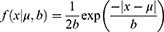
where f(x) is dependent on parameter μ, related to the peak of events, and b is a scale parameter.

A major issue with exponential models is the need to enter the time of the peak in infections. An example is shown in Figure 1, in which estimates of infections are calculated with different peak dates. Infections with peaks at 40 days, 45 days and 50 days show total infections rising from 140,000 to 620,000 and then to 2.7 million. This represents a range of more than one order of magnitude; when doubling of cases occurs every day the totals can increase to impossibly high levels.

Figure 1 Example of exponential growth with various days to peak.

SIR (Susceptible-Infected-Removed) and Related Models

In 1927, Kermack and McKendrick developed a mathematical model for infectious diseases based on the number of people infected, the recovery and death rates.² This model where populations are assigned to different “compartments” has been extended to different and additional segregation including SIS (Susceptible Immune Susceptible) and SIRD (Susceptible Infectious Recovered Deceased). Recently, the method has been used to describe the COVID-19 outbreak in South Korea.³ The rate of transmission from person to person is highly heterogeneous, with population density, behaviour, mitigation practices, and seasonality having large impacts on the model outputs. The substantial number of potential variables, many of which are unknown at the start of a disease outbreak, and the fact that R_t/R₀ infection rates are estimates and cannot be measured directly in large samples can lead to inaccurate estimates for the number of cases and deaths.

Gompertz Distribution Models

The S-shaped curve of the Gompertz distribution more accurately describes infectious disease outbreaks than the exponential model. The equation is:

where f(t) is the distribution, a is the upper asymptote, b is a growth rate, c defines the point of inflection and t is time.

A major input to the model is the parameter a, which for infectious diseases is the total number of cases or deaths. The model is very sensitive to the growth rate and does not forecast the inflection point, requiring estimates for these two parameters. A priori iterative solutions to the equation can have wide error margins. This can be seen in Figure 2, in which the distribution is used with UK COVID-19 data. Various estimates were used to give close correlation of the model to actual data in the early stage of the disease outbreak; however, there is wide variation in the estimates.

Figure 2 Examples of forecasts based on 20-day input data after 50 deaths.

Lee et al used data published between 22 Jan 2020 and 9 April 2020 for 50 countries and developed a Bayesian hierarchical model using Gompertz distributions, with integration of the global data to estimate COVID-19 infections. The authors stated that combining data from various counties gave a more accurate model for the global infection rate than for individual countries.⁴

Skew-Reflected-Gompertz Distribution

This model is applicable to infectious disease outbreaks in which there is a difference between the growth and decline phases. Again, when solving for total cases, it is very sensitive to the primary input parameters, with the addition of estimates for variables needed to describe the decline in infections and deaths. The equation is:

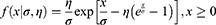
where σ and η are scale and shape parameters.^5,6

The authors are not aware of infectious disease studies that use the asymmetric Gompertz model.

Novel Model

The Novel Difference Model

This model was developed by the authors in 2020 during an investigation of COVID-19 cases and deaths for various countries. After using exponential and Gompertz distributions to generate models, it became clear that a critical requirement for any model would be an accurate determination of the date of peak infections. In all infectious diseases, there is a peak level of infection, and the difference model is based on forecasting the date for peak infections prior to its occurrence. During the early stages of the COVID-19 outbreaks, there were several databases published for cases and deaths. The UK Office for National Statistics (ONS) recorded deaths attributed to SARS-CoV-2 with data reported by hospitals, care homes, primary care trusts and others.⁷ Data from this web site was downloaded on the 31st July 2020. The UK COVID-19 data from the first death and for the next 30 days are shown in Table 1.

Table 1 UK COVID-19 Deaths. Johns Hopkins University (Worldometer) Data

The data indicate continued growth of both daily cases and total cases. Also shown is the rate of change of daily deaths. When this day-to-day change of deaths is plotted it can be seen that at some point the distribution crosses the abscissa, such that a declining but positive daily change becomes negative. This occurs when the change in daily cases moves from growth phase to decline phase and occurs on the peak date of the outbreak, which is the most critical, but unknown, parameter.

Owing to the low number of cases at the start of this outbreak, the rate of change data are typically unstable up to day 10. Initially, an arbitrary date for the model was chosen when total deaths exceeded fifty. Subsequent modelling with different start points helped quantify error rates. A plot of the data from day 13, when total deaths first exceeded 50, and for the next 20 days, is shown in Figure 3.

Figure 3 Chart of daily change of reported deaths with linear regression.

The linear equation describing the trend has slope −0.0125 and intersects the abscissa at 40.1 days. Hence, the peak day for the number of deaths is 40.1 days from the first death, in this case the 12th April 2020. The linear equation is:

(1)

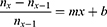
where n = number of deaths; x = day number; m = gradient of linear function; and b = the intercept with the ordinate when y = 0

The inflection point where growth of deaths peak occurs at:

(2)

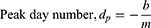
The actual peak day is derived from the date that the 7-day moving average of reported deaths is a maximum. The comparison of forecast to actual date is shown in Table 2.

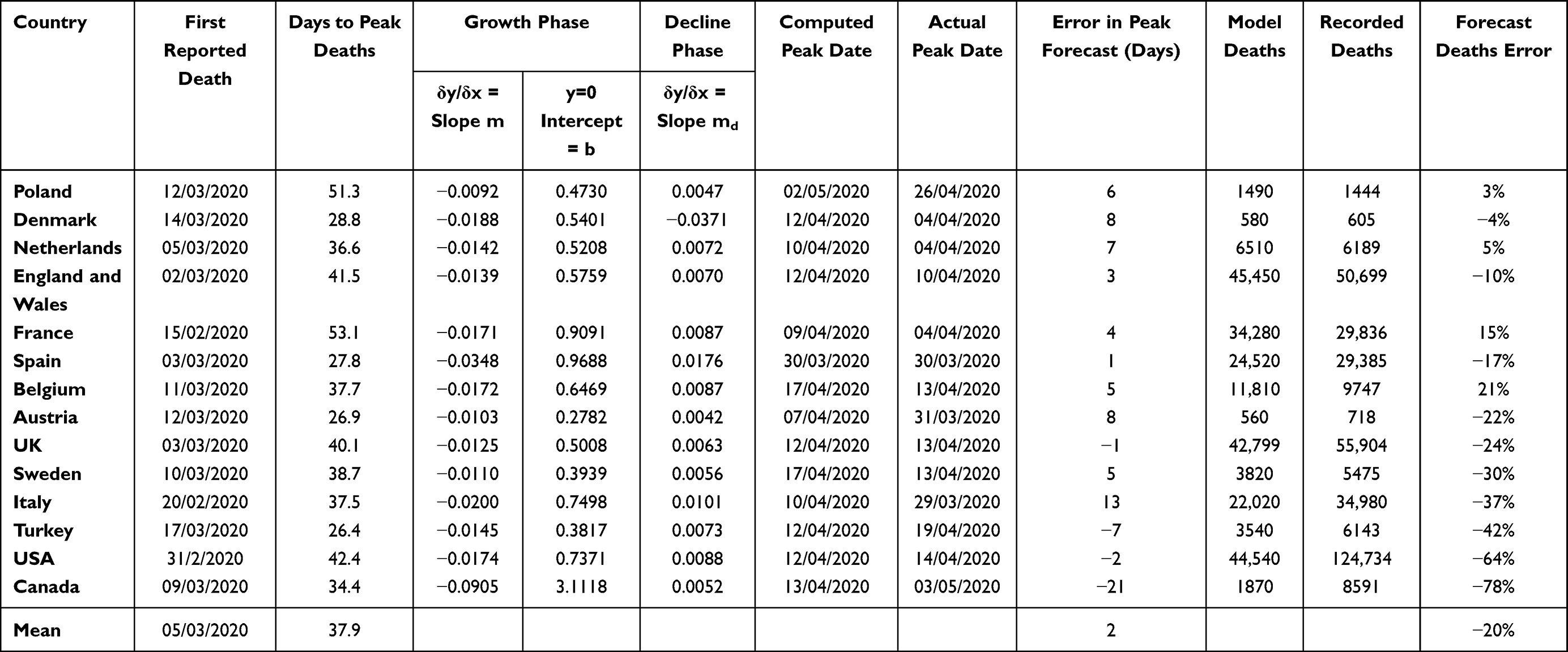Table 2 COVID-19 Mortality: Asymmetric Model Parameters and Forecasts Based on JHU Worldometer Reported Data and Office for National Statistics for England and Wales

The estimated deaths for day x is:

(3)

The total deaths to day X is:

(4)

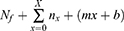
where N_f is the total deaths up to the start of the forecast.

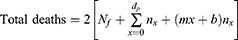
The total deaths to the peak date is:

(5)

For the symmetrical model, the total deaths are twice the number of deaths to peak date:

(6)

A chart of the symmetric difference model with ONS data is shown in Figure 4. This shows the original data for the 1st to the 50th death, the data for the next 20 days used for the model, and the forecast. It predicts the peak date a few days earlier than the actual date and does not describe accurately the slow decline in cases. The cause of the slow decline was not known and so a search for historical data for the trajectories of infection was conducted. The results are shown and discussed in the next section.

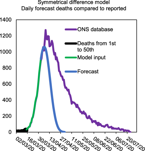Figure 4 Model input data for 20 days after 50th death and output compared to actual data.

The Asymmetrical Difference Model

The ONS published comprehensive data for excess winter deaths attributed to ILI for the years 1999 to 2014.⁸ A graph of these data is shown in Figure 5.

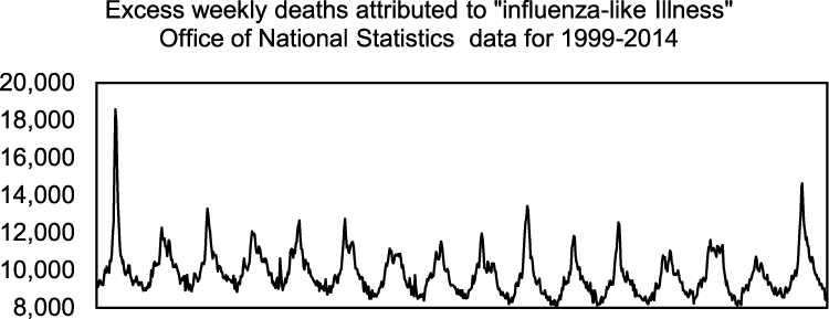Figure 5 A chart created from ONS data for Influenza like illness (ILI) for the years 1999–2014 showing the trajectory of excess deaths.

Analysis was carried out on these data and charts were created for each year. These are consolidated in Figure 6. The period for growth of deaths from the beginning to the peak and from the peak to the end of the outbreak were estimated from the data and the ratio between time to decline versus time to “peak” calculated; the results shown in Table 3. The data for some years demonstrated two or more peaks. It was assumed that this represented multiple outbreaks with different cold or flu viruses. In order to model a single viral infection, the years where there was a single peak were used to create an average rate of decline.

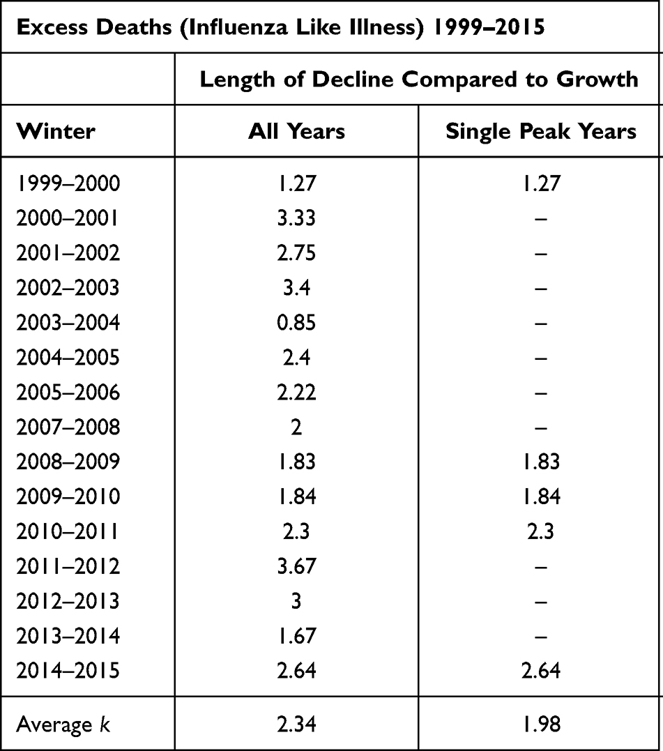Table 3 Ratio of the Growth and Decline Phases of Influenza Like Illness Outbreaks

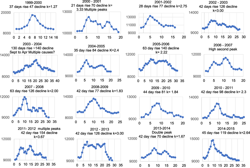Figure 6 Details of weekly ILI excess deaths with estimates for the number of days to the peak and for the decline to normal levels. X axis data is Week number after outbreak.

The symmetrical difference model was modified to describe the slow decline by adding a term to the equation using a separated linear equation for declining daily difference in deaths. A chart based on the ONS model input data and the linear slope depicted in Table 3 (k = 1.98) is shown in Figure 7.

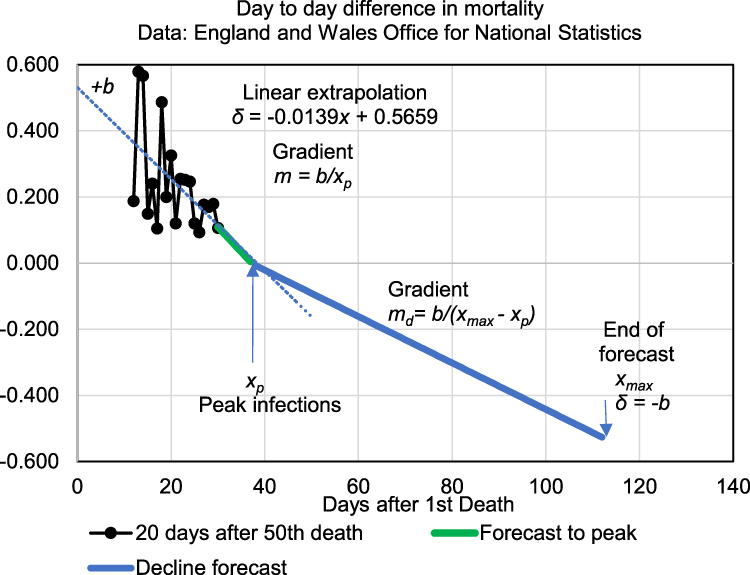Figure 7 Diagram of parameters for the asymmetric model.

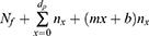
From Figure 7, the model for declining cases is given by:

where m_d is the slope of the declining linear function; b is the intercept when x = x_max; and x_p is the day number at which peak infections occur, ie

in which k is the time dilation for declining infections.

Hence,

It follows that,

(7)

where n is the number of deaths and x is the day number.

Therefore,

Total mortality can then be calculated from:

where N_f = total deaths up to the end of the forecast and x_max is the ending date of the forecast.

A comparison of the trends for cumulative events, daily events and the day-to-day difference rate for the Gompertz model, the symmetric difference model and the final asymmetric model are shown in Figure 8.

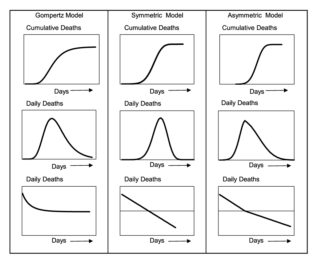Figure 8 A comparison of cumulative, daily and daily change in mortality for three models.

The asymmetric model was used with the Johns Hopkins University (Worldometer) data for the deaths reported in the 30 days after the first death shown in Table 1. The forecast for cumulative deaths is shown in Figure 9. The forecast shown in blue on the chart is based on the recorded data shown in the 20-day period after the 50th death shown in green. The forecast for total COVID-19 deaths is 45,610 compared to 50,699 recorded on 30th June 2020.

Figure 9 Comparison of model and total deaths reported on 30 June 2020.

The forecast and actual data for daily deaths are shown in Figure 10, from which the forecast tracks the recorded trajectory closely.

Figure 10 Comparison of model to actual daily deaths reported on 30 June 2020.

Asymmetric Model Forecasts for Death Rates for Other Countries

Input data for the UK and other countries were obtained from the Johns Hopkins University Worldometer (JHU) website.⁹ This database consolidated inputs from various countries around the word with daily updates that included new cases, new deaths and additional data computed for cases/deaths per million population, etc. Table 3 shows the model parameters and outputs for a number of countries along with the error of the forecasts compared to JHU reported data up to 30 June 2020.

The accuracy of the model is dependent on the identification of the peak for daily deaths prior to its occurrence. The smallest error in calculating the peak data is one day in the case of Spain. For 11 of the 14 countries the error was 7 days or less.

The mortality rates predicted by the model compared with reported data are quite accurate with errors ranging from +3% for Poland and with errors less than ± 25% for 9 of the 14 countries. For all countries, the mean error was and underestimation of 20%. Twelve of the 14 estimates have errors less than 50%. The largest error, (for Canada), was −83%, and an underestimation for the USA of −64%. The cause of these excess deaths could not be deduced from the model or input data but may be identified at a future time. The JHU database generated an error in the forecast for the UK of −24% which is significantly different from the error for England and Wales based on the ONS report of −10%. A study by Oxford University identified an issue with the Public Health England (PHE) data where deaths from any cause were listed as COVID-19 deaths if the person had a positive test at any time prior to the death. In contrast, the ONS data were compiled from cases where COVID-19 was listed on the death certificate.¹⁰ As with Canada, the USA and some other countries, there is significant under estimation of recorded deaths. The cause of these differences cannot be identified.

Limitations of the Model

The forecasts are dependent on the input data, and there is published evidence that the methods and definitions adopted by some countries resulted in incorrect counts for both deaths and cases. Evidence for this is shown by the forecasts for England and Wales using death certificate records and those for the UK where other and varying methodologies were adopted.

The fundamental goals of the model were to give estimates of deaths based on the limited data available during the early stages of infections, to allow rapid determination of the risks and allow optimum governmental and health service responses. The threshold of 50 deaths was selected since the daily change was stable for most countries studied from that point onwards. In some countries, the death rates were so low that the change in daily cases never stabilised, resulting in the linear growth parameter being near zero or positive growth. An example of a country for which the algorithm failed to generate data is Japan. Although this would appear to be a serious weakness of the model, in fact it demonstrates that when the model fails there are very low levels of deaths during the early phase and during the outbreak.

It was not possible to generate estimates for SARS-CoV-2 mortality for many countries during the period of this study. These generally were countries in the southern hemisphere. This was since the outbreaks were occurring later than in the northern hemisphere, (in the summer months) and the majority of cases and deaths occurred later than the cut-off date used for this study (30th June 2020).

Conclusions

Using the “asymmetric difference model” to forecast deaths gives accurate estimates, with a mean error of −20% for 14 countries studied. The lowest error rates were +3% for Poland, −4% for Denmark and +5% for the Netherlands, and the errors for twelve countries were less than 50%. The error was −24% for the UK. However, the model generated an error of −10% for England and Wales, which represents 89% of the UK population. The database used for the England and Wales model was compiled and published by the ONS using death certificate records. In contrast, the data for the UK were published by JHU from information supplied by the UK. This included the data for England provided by PHE which were found to include deaths from causes other than COVID-19. In all countries, the model accurately predicted very low levels of COVID-19 deaths compared with country populations. The model gives these results with very limited data, typically published during the first 30–40 days of an outbreak of disease and should provide accurate forecasts to allow optimum planning by health services and government agencies.

References

1. Dontwi I, Obeng-Denteh W, Andam E. A mathematical model to predict the prevalence and transmission dynamics of tuberculosis in Amansie West District, Ghana. Br J Math Comput Sci. 2014;4(3):402–425. doi:10.9734/BJMCS/2014/4681
2. Kermack WO, McKendrick A. A contribution to the mathematical theory of epidemics. Proc R Soc Lond Ser A. 1927;115(772):700–721.
3. Kim S, Jeong YD, Byun JH, et al. Evaluation of COVID-19 epidemic outbreak caused by temporal contact-increase in South Korea. Int J Infect Dis. 2020;96:454–457. doi:10.1016/j.ijid.2020.05.036
4. Lee SY, Lei B, Mallick BK. Estimation of COVID-19 spread curves integrating global data and borrowing information. medRxiv Prepr. 2020. Available from: http://arxiv.org/abs/2005.00662.
5. Contreras-Reyes JE, Maleki M, Cortés DD. Skew-Reflected-Gompertz information quantifiers with application to sea surface temperature records. Mathematics. 2019;7(5):1–14. doi:10.3390/math7050403
6. Werker AR, Jaggard KW. Modelling asymmetrical growth curves that rise and then fall: applications to foliage dynamics of sugar beet (Beta vulgaris L.). Ann Bot. 1997;79(6):657–665. doi:10.1006/anbo.1997.0387
7. Office for National Statistics. Deaths registered weekly in England and Wales, provisional [Internet]; 2020 [cited July 28, 2020]. Available from: https://www.ons.gov.uk/peoplepopulationandcommunity/birthsdeathsandmarriages/deaths/bulletins/deathsregisteredweeklyinenglandandwalesprovisional/weekending10july2020.
8. Office for National Statistics. Highest number of excess winter deaths since 1999/2000. Office for National Statistics [Internet]; 2015 [cited April 6, 2020]. Available from: https://www.ons.gov.uk/peoplepopulationandcommunity/birthsdeathsandmarriages/deaths/articles/highestnumberofexcesswinterdeathssince19992000/2015-11-25.
9. Johns Hopkins Univ. Worldometer. COVID - 19 Coronavirus Pandemic [Internet]; 2020 [cited April 6, 2020]. Available from: https://www.worldometers.info/coronavirus/.
10. Howden D, Oke J, Heneghan C. Death certificate data: COVID-19 as the underlying cause of death [Internet]. Centre for Evidence-Based Medicine; 2020 [cited October 25, 2020]. Available from: https://www.cebm.net/covid-19/death-certificate-data-covid-19-as-The-underlying-cause-of-death/.
© 2023 The Author(s). This work is published and licensed by Dove Medical Press Limited. The
full terms of this license are available at https://www.dovepress.com/terms
and incorporate the Creative Commons Attribution
- Non Commercial (unported, 3.0) License.
By accessing the work you hereby accept the Terms. Non-commercial uses of the work are permitted
without any further permission from Dove Medical Press Limited, provided the work is properly
attributed. For permission for commercial use of this work, please see paragraphs 4.2 and 5 of our Terms.
Recommended articles
COVID-19 and Saudi Arabia: Awareness, Attitude, and Practice
Fawzy MS, AlSadrah SA
Journal of Multidisciplinary Healthcare 2022, 15:1595-1618
Published Date: 26 July 2022
A Pilot Study of 0.4% Povidone-Iodine Nasal Spray to Eradicate SARS-CoV-2 in the Nasopharynx
Sirijatuphat R, Leelarasamee A, Puangpet T, Thitithanyanont A
Infection and Drug Resistance 2022, 15:7529-7536
Published Date: 21 December 2022
Clinico-Epidemiological Profile of COVID-19 Patients with Omicron Variant Admitted in a Tertiary Care Center, South India
Ethirajan T, Natarajan G, Velayudham R, Jayakumaran P, Karnan I, Rajendran K, Doraisamy S, Chenakeswarar Sridhar S, Kumaran P, Kamaraj K, Kandasamy A, Natarajan M
International Journal of General Medicine 2023, 16:185-191
Published Date: 17 January 2023
Distinct Features of Vascular Diseases in COVID-19
Ceasovschih A, Sorodoc V, Shor A, Haliga RE, Roth L, Lionte C, Onofrei Aursulesei V, Sirbu O, Culis N, Shapieva A, Tahir Khokhar MA, Statescu C, Sascau RA, Coman AE, Stoica A, Grigorescu ED, Banach M, Thomopoulos C, Sorodoc L
Journal of Inflammation Research 2023, 16:2783-2800
Published Date: 6 July 2023
Re-Emerging COVID-19: Controversy of Its Zoonotic Origin, Risks of Severity of Reinfection and Management
Chala B, Tilaye T, Waktole G
International Journal of General Medicine 2023, 16:4307-4319
Published Date: 20 September 2023