Back to Journals » Clinical Epidemiology » Volume 7
Using multiple imputation to deal with missing data and attrition in longitudinal studies with repeated measures of patient-reported outcomes
Authors Biering K, Hjollund NH ![]() , Frydenberg M
, Frydenberg M
Received 4 August 2014
Accepted for publication 18 November 2014
Published 16 January 2015 Volume 2015:7 Pages 91—106
DOI https://doi.org/10.2147/CLEP.S72247
Checked for plagiarism Yes
Review by Single anonymous peer review
Peer reviewer comments 4
Editor who approved publication: Professor Vera Ehrenstein
Karin Biering,1 Niels Henrik Hjollund,2,3 Morten Frydenberg4
1Danish Ramazzini Centre, Department of Occupational Medicine – University Research Clinic, Hospital West Jutland, Herning, Denmark; 2WestChronic, Regional Hospital West Jutland, Herning, Denmark; 3Department of Clinical Epidemiology, Aarhus University Hospital, Aarhus, Denmark; 4Section of Biostatistics, Department of Public Health, Aarhus University, Aarhus, Denmark
Objective: Missing data is a ubiquitous problem in studies using patient-reported measures, decreasing sample sizes and causing possible bias. In longitudinal studies, special problems relate to attrition and death during follow-up. We describe a methodological approach for the use of multiple imputation (MI) to meet these challenges.
Methods: In a cohort of patients treated with percutaneous coronary intervention followed with use of repetitive questionnaires and information from national registers over 3 years, only 417 out of 1,726 patients had complete data on all measure points and covariates. We suggest strategies for use of MI and different methods for dealing with death along with sensitivity analysis of deviations from the assumption of missing at random, all with the use of standard statistical software. The Mental Component Summary from Short Form 12-item survey was used as an example.
Conclusion: Ignoring missing data may cause bias of unknown size and direction in longitudinal studies. We have illustrated that MI is a feasible method to try to deal with bias due to missing data in longitudinal studies, including attrition and nonresponse, and should be considered in combination with analysis of sensitivity in longitudinal studies. How to handle dropout due to death is still open for debate.
Keywords: PCI, SF-12, nonparticipants, nonrespondents
Introduction
An inevitable everyday challenge for epidemiologists is missing data. We think of missing data as data that we planned to collect but did not get. This poses challenges for both reliability and validity of the estimates. Especially, nonparticipation (invited patients who never participated in the study) and attrition (loss during follow-up of participants who initially were in the study) imply problems in longitudinal studies. Nonparticipants often differ from the source population with respect to disease severity as well as other covariates, for example, sex, age, and education.1
Attrition occurs in most clinical trials and observational studies if they involve more than one measurement point. Especially in clinical epidemiology, changes in disease severity or symptoms may influence patient participation.1 During follow-up, the participants may be unwilling or too ill to continue participation, they may move and fail to report their new address, or they may even die, although the latter may not be regarded as attrition.2 The opposite mechanism may operate if the patient considers himself to be marginal with respect to the aim of the study (eg, too few symptoms or symptoms primarily related to comorbidity). Patients may find participation tedious and time-consuming, and even comorbidity or life events may play a role unknown to the researchers. However, the patient characteristics or the mechanism behind attrition is seldom reported.3 The reasons why participants drop out are, however, usually unknown, and consequently, evaluation of the role, and even the direction, of bias may be speculative.
Specific analytical problems arise when the patients die during follow-up. In this case, we do not consider it as a missing data problem, as we are not interested in patient-reported outcomes, when patients are dead. In most studies, patients who die during follow-up are simply excluded from the analysis, but results from these studies are often too optimistic.4 In other approaches, the “worst” value is assigned to the patient-reported outcomes variable for patients who die during follow-up,5–7 or an indicator of having been alive at next point of measurement is introduced.8
Both nonparticipation and attrition may introduce selection bias if the reason for is related to the outcome of interest.9 The problem with missing data is accentuated by the fact that most statistical methods (eg, regression models) will exclude cases with incomplete observation of any covariate or outcome – a complete case analysis. Linear mixed models are often used in studies with repeated measurements and will, in some cases, give unbiased estimates by just analyzing the observed data; hence, you will not need to impute the missing data. However, this will, in general, require that the model involve all the variables needed to make the missing-at-random (MAR) assumption valid, and will hold only if the outcome has missing values, not if the covariates have missing values. An unbiased linear mixed model also requires that attrition is not related to the outcome. A thorough introduction to linear mixed models and missing data can be found in Verbeke10 and Twisk.11
Types of missing data
We will briefly explain the different types of missing data in the following. We say that the data is missing completely at random (MCAR) if the chance of observing data is identical for the data that we in fact observed and the data we did not observe. In the case of MCAR, analyses of complete cases will introduce no bias but will decrease the sample size and hence, the precision of the estimates. However, in most cases, the risk of missing data is related to other variables (observed or unobserved); that is, if the data are not MCAR, then analyses based only on complete cases may cause bias. Now suppose that, given all we have observed about a person, the risk of missing a specific observation is independent of the actual value of that observation (eg, the risk that data is missing is independent of the values of the unobserved variables, given the observed variables), then we will say that the data are MAR. The keystone in the missing data theory is that if data are MAR, then it is theoretically possible to make valid and efficient inference based on the collected data (but not by a complete case analysis).12 Finally, the data are said to be missing not at random (MNAR) if they are neither MCAR nor MAR. We will by no means provide a full introduction to the topic but refer to Sterne et al, White et al, and Carpenter et al for further details.13–15
Imputation
In recent decades, different approaches have been developed to deal with missing data, but we will focus on imputation. The idea behind imputation methods is that as we know how to analyze the data if there were no missing data (planned analysis), and if we could fill in (impute) the missing data, then we could just analyze this imputed dataset. The simplest form of imputation is single imputation where a missing observation for a specific variable for each person is replaced by a reasonable value such as, for example, the mean of the observed values for that variable or as “last observation carried forward” (missing values are replaced by the last observed value of that variable) in longitudinal studies. Although estimates based on single value-imputed data are unbiased if the imputation model is correct, this method will not supply valid standard errors, confidence intervals, or P-values. In multiple imputation (MI), we create several (m) imputed datasets, in which we, in each set, replace missing observations with random values from a statistical model based on distributions in the observed dataset and underlying assumptions on the nature of the missing data.13,14 After this, we analyze each of the imputed datasets by the planned analysis to obtain m sets of estimates and corresponding standard errors. The final estimates are found as the average of the m sets of estimates and the standard errors by applying a simple formula called Rubin’s rule.12 The obtained standard error incorporates the two sources of uncertainty, the standard error of the estimate for each of the m datasets and the random variation between estimates derived from different imputed datasets. If data are MAR and the models used in the imputation are chosen adequately, MI will give a valid inference.13,14 As it is theoretically impossible to verify the assumption of MAR, the MI analysis should be accompanied by sensitivity analyses that illustrate how realistic departures from MAR would affect the results.
When patients die during follow-up, we do not consider it as a missing data problem because patient-reported outcomes are irrelevant when patients are dead. In most studies with repeated measurements, patients who die during follow-up are simply excluded completely from the analysis, but results from these studies are often too optimistic.4 In other approaches, the “worst” value is assigned to the variable for patients who die during follow-up,5–7 or an indicator of having been alive at the next point of measurement is introduced.8 Kurland et al discuss the importance of choosing the model according to the aim of the study,16 while Harel et al and Ning et al give examples of MI in simulated settings.17,18
The aim of the present paper is to describe a specific application of MI exemplified in a concrete follow-up study with numerous measurement points and external data from national health and socioeconomic databases. The paper focuses on the challenges of missing data in the study, the assumptions and methods behind MI, and the use of sensitivity analysis. We did not aim to compare different approaches to deal with missing data but rather to provide a solution accessible to the majority of epidemiologists by the use of standard statistical software.
The analytic aim of the follow-up study used as the example was to describe the long-term course of self-reported health in a cohort of patients treated with percutaneous coronary intervention (PCI), using repeated measurements of the Short Form 12-item survey (SF-12) component summaries of mental and physical health,19 along with differences in the course of self-reported health with respect to left ventricular ejection fraction (LVEF), indication for PCI, age, sex, and educational level using a linear mixed effect model. The specific results corresponding to these analytic aims are presented in a separate paper.20
Materials and methods
Materials
We used data from a study of patient-reported outcomes in 1,726 consecutive patients treated with PCI at Aarhus University Hospital, Denmark. For a period of 36 months, patients were repeatedly followed with questionnaires, to establish eight fixed measure points during follow-up (1 month, 3 months, 6 months, 12 months, 18 months, 24 months, 30 months, and 36 months after PCI). The mode of data collection was a combination of mailed and emailed questionnaires, depending on the patients’ preference. The patients provided their e-mail addresses voluntarily. The measure points were established to reflect the most precise timing of the answer to the questionnaire based on an algorithm that used the actual date of the answer compared to the date of the PCI procedure, rather than the number of the questionnaire.
Patients received up to two reminders if they did not respond within 2–3 weeks after each questionnaire. Patients who did not respond after the two reminders were not sent the following questionnaires. At the end of the study, we mailed a final questionnaire to all patients who were still alive, including those who had stopped answering during follow-up, but had not contacted us with a specific denial.
The course of the data collection is presented in Table 1. The cohort includes 1,726 patients who provided 7,872 questionnaires covering the eight measurement points. Seventy-four patients died during follow-up. The patient’s response category could change over time; for example, one could be classified as a nonrespondent in the beginning of the study, but return the initial questionnaire later than requested, and then be classified as a returnee. After that, the same patient could stop answering further questionnaires and thus be classified as a dropout. The data collection is described in detail in Table 1 (upper part).
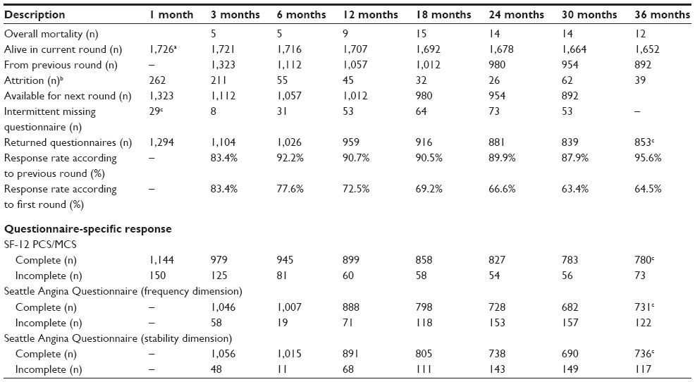 | Table 1 Response patterns and attrition in a cohort of patients treated with PCI at Aarhus University Hospital, Skejby (N=1,726) |
In this paper, we focus on the repeated measurements of SF-12 component summaries. The SF-12 data were scored into the two component summaries: Mental Component Summary (MCS) and Physical Component Summary (PCS). In this scoring, persons who had not completed all 12 items were categorized as missing.19 We also included repeated measurements of two heart-specific dimensions from the Seattle Angina Questionnaire (SAQ), namely “stability” (SAQs) and “frequency” (SAQf).21 SF-12 scoring started 1 month after PCI, while SAQs and SAQf started 3 months after PCI (Table 1, lower part).
Other information used in this study from the questionnaire at 3 months were educational level (low, intermediate, or high from International Standard Classification of Education)22 and leisure time physical activity (four categories: <2 hours per week, 2–4 hours per week, >4 hours per week, or >4 hours per week and heavy).
In Denmark, accurate and unambiguous linkage of registries and clinical databases at the individual level is possible due to a unique central personal registry number assigned to each Danish citizen at birth and to residents on immigration.23 Supplementary to the questionnaires, we had access to the following register-based data:
- Sex and day of birth were provided from the Danish Civil Registration System along with information about the exact day of death, for those who died during follow-up.
- Comorbidity calculated as Charlson Index24 was provided from the Danish National Patient Registry.25 Charlson Index was categorized into 0, 1–2, and >3.
- Body mass index (BMI), smoking status, indication of the PCI (acute or elective), and LVEF were available from a clinical database, West Denmark Heart Registry.26
- Transfer payment groups (TPGs) were provided from the Danish Register for Evaluation of Marginalization (DREAM).27 DREAM contains information about income sources at a weekly basis, and we used the information for the week before PCI and at each time point of the questionnaires. For each week, each patient was categorized into one of the five categories: 1) working or unemployed, 2) receiving health-related benefits, 3) early retirement, 4) normal retirement, and 5) dead or emigrated. If patients did not report their educational level, categorizations were based on the patients’ membership of a trade union, which was available from DREAM (available for 512 patients out of 682 missing). The register-based data were complete for all patients, but in the West Denmark Heart Registry, BMI was missing in 76 cases (4.4%) and smoking habits in 70 (4.1%) cases. From self-reported height and weight, we were able to create an additional 34 BMI values, while self-reported smoking status added 48 additional values to the data from the clinical database. The data on TPGs and date of death were added to the dataset because we knew we had missing data, and we intended to use these as additional information in the imputation models.
During the data collection, some patients skipped single items, some returned a scheduled questionnaire later than requested, some stopped answering the questionnaires, and some died during follow-up. This resulted in several kinds of missing data, item, scale score, and questionnaire levels, along with attrition and total nonparticipation. Figure 1 illustrates different types of response in a simplified overview. All together, 46 different response patterns were identified in our cohort on the questionnaire level, not taking missing items and deaths into account. In reality, nearly each individual may have his or her pattern of missing data, when taking all items in a longer questionnaire into account.
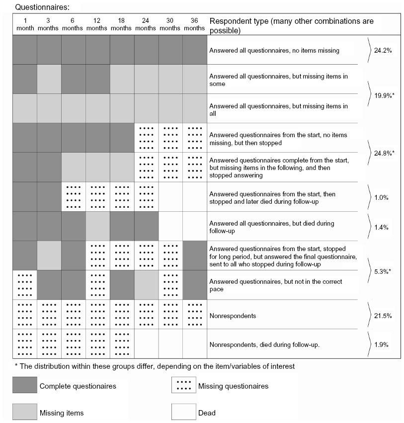 | Figure 1 Exemplified overview of some respondent types in a follow up study of PCI patients. |
Baseline characteristics including missing data distributed on whole-course respondents, dropouts, returnees, and nonrespondents are described in Table 2. We defined whole-course respondents as patients who responded to all questionnaires (n=761). Respondents who dropped out were defined as people who stopped answering during follow-up, including those who answered only the first questionnaire (n=470). In the group of respondents who dropped out, 42 patients died during follow-up. Returnees were patients who completed parts of the study, but not at the scheduled pace, resulting in missing questionnaires (n=92). This group included the dropouts that were approached again at the end of the study. Nonrespondents were defined as patients who did not return any questionnaires at all (n=403). The nonrespondents also included the 141 patients who were never invited to take part in the study because they had a hidden address. In the group of nonrespondents, 32 patients died during follow-up.
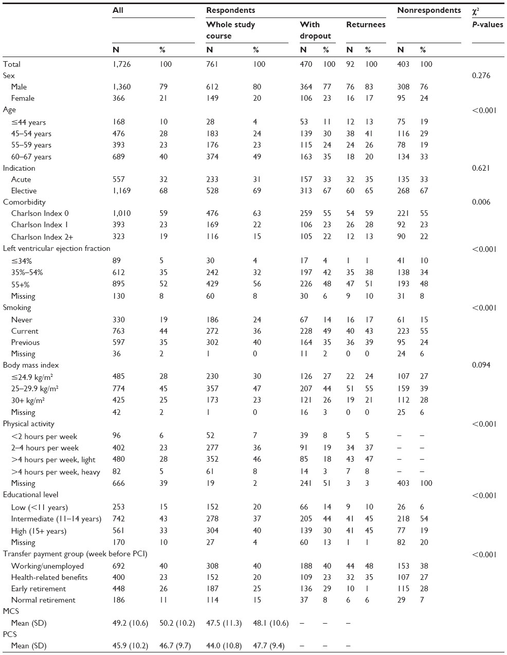 | Table 2 Characteristics of response types |
These response types can also be identified in Figure 1, where the upper three rows are patients who completed the whole study; the following four rows are examples of patients who stopped during follow-up, then two rows with returnees, and the two bottom rows with nonresponders.
In the SF-12 component summaries, several respondents skipped one or more items, resulting in a missing score (Table 1, lower part), and in the SAQ, a considerable number of respondents skipped the questions, possibly because they did not experience any symptoms. All together, only 470 patients completed all eight questionnaires with all SF-12 items filled in, and out of these, only 417 had complete data regarding smoking, BMI, LVEF, physical activity, and educational level, as required for an unbiased complete case analysis. If we used the complete cases only, a considerable number of patients would be excluded.
Patients who were nonrespondents differed from the respondents who completed the whole study course, by being more often women, younger, and more often treated with acute PCI. They suffered more often from comorbidities and had unhealthier lifestyle, in terms of smoking habits and BMI. The patients who were nonrespondents due to hidden address were similar to the respondents, except from that they were slightly younger and more often women (data not shown). Patients who dropped out differed from the patients who completed the whole study course in the same aspects as those between nonrespondents and respondents. In addition, they were less physically active. Like the nonrespondents, the patients who dropped out were more often temporarily or permanently out of work. The returnees were similar to the patients who completed the whole study course, except that they were, in general, younger and thus more often treated acutely; they were more often current smokers and slightly overweight. They were slightly better educated, perhaps because of their younger age.
The nonrespondents had a higher mortality than the respondents. Also, they were more often temporarily or permanently out of the work (except from normal retirement, which was most common among respondents), and this pattern applied to all time points during follow-up. During follow-up, 74 patients died (32 nonrespondents and 42 respondents). The patients who died during follow-up differed from those who were lost to follow-up for other reasons; they were older and had a lower LVEF. They also had more comorbidity. Many of those who died had left the workforce permanently already from the beginning of the study.
We concluded that there were many differences between respondents and nonrespondents, between whole-course respondents and respondents who dropped out, as well as between patients who died during follow-up and those who dropped out for other reasons. These differences are presumably all related to health and therefore, we assumed that results based on complete cases would most likely be biased. The direction of the bias would be an overestimation of self-reported health, as this was strongly prone to be related to most of the variables about which nonrespondents, patients who dropped out, and dead patients differed from the whole-course respondents.
In the case of MAR, we can make assumptions about relations to other variables in our dataset, and consequently be able to predict the missing values.13,14,28 Since we were aware of several characteristics related to both nonresponse and attrition, of which many were complete for all patients, our missing data could be MAR, and thus suitable for MI. To improve our approach even further, we used the external data on date of death and TPG, even though these were not used in our planned analysis.
To build the models of the variables of interest in MI, we used the baseline characteristics that we found related to nonresponse and attrition and data related to the level of the variable in focus as recommended by Fielding et al.29 We took advantage of the longitudinal data structure in the models and used the previous and the following measurement of the same score in the models. In many cases, imputation models are based on related measures but not on the same measure in a previous or following questionnaire.
Methods
Generating the imputed datasets: specifying the models
In order to impute a missing value, one has to specify a stochastic model for each variable with missing values. Although some statistical programs may carry out MI using all available variables in standard models without any insight into the underlying mechanism, the use of specific equations is preferable.13 This involves several decisions: which type of model is appropriate, should the variable be transformed, which variables should be used as explanatory variables, etc. These are exactly the same considerations as when one is formulating a regression model in an ordinary statistical analysis. But there is an additional requirement to the imputation models if they are to be used to give unbiased estimates under the assumption of MAR: whether or not the variable is actually observed should be independent of the actual value, given the explanatory variable included in the model.
We will illustrate the imputation models with some examples (a list of all the 35 models is given in Table S1 and Figures S1–S3), starting with SF-12 MCS, which is of primary interest in this study. The MCS at time t was a model of normal linear regression given by the following equation.

where t – 1 and t + 1 indicate the previous and the following questionnaires, respectively. Here, we use the convention that t – 1 does not exist for the first questionnaire and t + 1 does not exist for the final questionnaire. Deadt+1 is 1 if the person died in the interval from t to t + 1. Note that TPG and Comorbidity are categorical variables indicated by asterisks (*). In other words, the MCS is assumed to depend on the previous and following MCS scores, the previous and present SAQs and SAQf scores, the present TPG status, the baseline characteristics (Age, Sex, LVEF, Indication for PCI, and Comorbidity), and on whether or not the person died before receiving the following questionnaire. Knowing the variables on the right side can ensure independency between the value on the left side and whether this value is observed. If this is true, the estimates calculated based on these MIs are unbiased. Two comments are needed here. First, we used the external data on income source at time t, as knowing this information makes the assumption of conditional independency between the MCS value and missingness more plausible. Second, we have introduced an indicator for death before the next questionnaire. This roughly means that we have a separate level of the MCS for those who died before the next questionnaire.
The SAQs score was modeled by an ordered logistic regression based on the following equation.

This equation is similar to that for the MCS, but here we did not include an indicator for death before the next questionnaire. We were forced by the data to do this, as there, for several of the time points, was no observed variation in the SAQs and SAQf score among those who died before the next questionnaire. As an example, 14 patients died in the interval of 18–24 months; in eleven, SAQs scores at 18 months were missing; and the remaining three had all the same SAQs score.
As an example of patient characteristics that do not vary over time, we considered BMI at baseline. This was modeled by the following linear regression.

In this situation, we used baseline characteristics such as age, sex, indication for the PCI, and prevalent comorbidity along with the patients’ rating of health in the first questionnaire. Note that here we do not need an indicator for death, as all patients were alive at the time of the first questionnaire.
We have decided that the fact that we do not have observed variables, for example, SF-12 scores, after a patient is dead is not a question of missing data; a dead patient cannot be assigned an SF-12 score. Rubin has discussed aspects of this in the setting of randomized trials.30 From this point of view, the patients’ death during follow-up is not a missing data problem. However, it can easily lead to a practical problem when we have to impute missing values prior to death. In the models, we have included both the previous and the subsequent questionnaires in the imputation model at a specific time point. However, if the person died before the subsequent questionnaire, then we do not have the information needed for the imputation. We have tried to handle this problem by using different strategies with or without an indicator in the model for patients who die before the next questionnaire combined with either treating missing observations after death as a missing data problem in the imputation and then resetting these to missing after the imputation, or assigning fixed values at the first questionnaire after death preceding the imputation and then resetting these to missing afterward. When assigning fixed values, we tried assigning both zero and a value close to the median of the score (50 if MCS/PCS and 100 in SAQs/SAQf). To summarize, we used the following five schemes:
- the observation after death treated as missing data, no indicator for death;
- the observation after death treated as missing data, with indicator for death;
- the observation after death assigned a fixed value (50/100), no indicator for death;
- the observation after death assigned a fixed value (zero), with indicator for death; and
- the observation after death assigned a fixed value (zero), no indicator for death.
For each scheme, we created 100 imputed datasets (m=100). We chose 100 imputations (m) as a conservative choice, as recent recommendations are to perform as many imputations as the proportion of missing cases in a study.14 Calculating this proportion of missing cases may be straightforward in studies with only a single or two measurement points, but in our longitudinal design, at least one variable in the dataset was missing in most patients, while in others (namely the nonrespondents), a large proportion of the variables of interest for the planned analysis are missing. As we added auxiliary variables in the imputation model, we reduced the proportion of missing data within each patient’s dataset, making calculations of proportions of missing data in the dataset arbitrary.
Generating datasets for the sensitivity analysis: specifying three different MNAR scenarios
The assumption behind valid estimation following MI is that data are MAR. We modified the dataset generated from MI in order to examine the consequences of departures from this assumption, for example, if data were missing in a patient who had poorer health than the imputation model could reveal under the MAR assumption. We reduced the imputed SF-12 component summaries because these were the focus of our planned analysis. The 141 patients who had a hidden address were omitted from this reduction, as they were similar to the respondents in respect to most baseline characteristics. The following three scenarios were generated: 1) reduction of ten points in all imputed values (corresponding to approximately one standard deviation, based on the general assumption that the mechanism behind missing data is related to lower self-reported health); 2) the same as scenario 1, but in nonrespondents, we subtracted an additional five points (based on the assumption that nonrespondents’ health was lower than the respondents’ health); and 3) the same as scenario 1, but in nonrespondents or patients with more than two comorbidities, we subtracted an additional five points (based on the assumption that patients suffering from other diseases would rate their health lower).
At this point, we had 21 different datasets because we had five variants of MI, each with an additional three variants of scenarios for sensitivity analysis along with the dataset with the observed data. When presenting the sensitivity analyses, we limit the presentation to imputation A together with the related variants of sensitivity datasets. We computed the four other schemes with variants of sensitivity analysis, and they revealed similar results.
We did not generate datasets with sensitivity scenarios to the two SAQ scores, as it was not possible to establish realistic scenarios, because the smallest possible reduction was 25 points to match one category in the stability dimension, and this would have a marked impact on the results. Other sensitivity analyses of other variables derived from MI are possible.
Analyzing the imputed data and the sensitivity datasets
Finally, we analyzed the dataset using a statistical model developed for an analysis of sex differences, which is presented in detail in the results paper.20 As in the presentation of the results for sensitivity scenarios, we present only the observed data, one variant of MI (Scheme A), and the related three datasets for sensitivity analysis.
All data management, computations, and analysis were performed in Stata/IC 12.1. The imputations and the analysis were performed using the MI/ICE suite in Stata with 100 imputations. Most other software packages provide similar possibilities. Estimates are given with 95% confidence intervals in square brackets.
Results
In the following, we present results related to the MCS only. The results related to results from the PCS are available in Table S1 and Figures S1–S3.
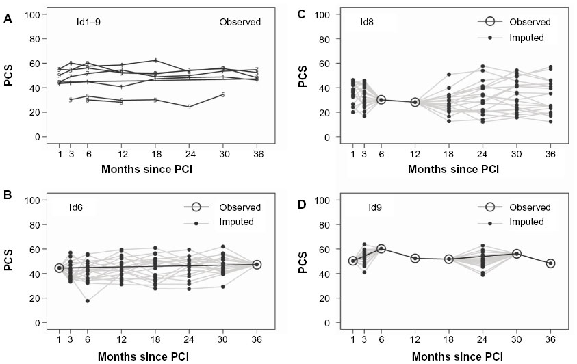
Figure 2A presents the observed data of the first nine patients in the dataset. Three patients (id1, id3, and id7) were whole-course respondents, and id2 was a nonrespondent (and thus not visible in Figure 2A with observed data). Some patients dropped out during follow-up (id4, id5, and id8), while some were returnees (id6 and id9). The figure also illustrates that in the observed data, some of the patients’ scores on the MCS varied nearly 20 points between two consecutive measurements (Figure 2).
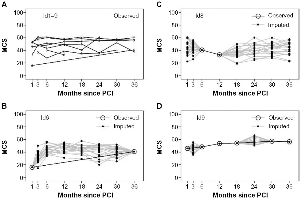 | Figure 2 Samples of nine patients observed data (A) and three different patients observed and imputed data (B–D). |
In Figure 2B–D, observed and imputed data (Scheme A) from patients id6, id8, and id9 are illustrated separately. For clarity, only the first 20 imputations are plotted. Patient id6 has observed data in the first and the last measurement, but the intermediate values are imputed. Patient id8 has observed data at 6 months and 12 months, but the remaining observations are imputed. In patient id9, two observations (3 months and 24 months) are missing, and compared to id6 and id8, the imputed data vary less because our imputation model used the previous and following observations, and these do not vary in this situation compared to, for example, the measurement at 24 months for id6 and id8, where the previous and following observations are missing (Figure 2).
After MI, the estimated mean component summary were approximately 1 scale point (~1/10 standard deviation) lower than in the observed data. The differences in the MCS were smaller during the first 6 months of follow-up, compared to the later follow-up period. The different schemes for handling missing data in the case of death (A–E) revealed very similar results (Figure 3A). Note that the y-scale is no longer 0–100, as in Figure 2. For the PCS, the differences were nearly stable over time (Table S1 and Figures S1–S3).
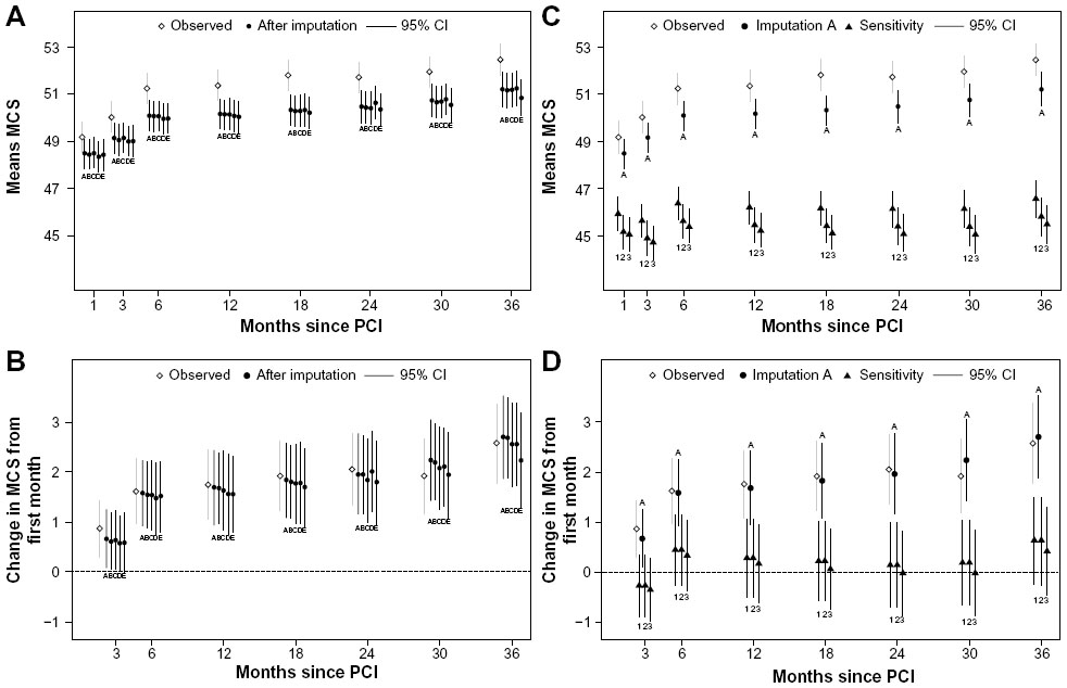 | Figure 3 Mean scores and mean changes of Mental Component Summary with observed data, variations of multiple imputation approaches related to dead (A and B), and sensitivity analyses (C and D). |
Looking at changes from the first measurement to each of the other measurements (Figure 3B), we found only minor differences between the observed data and the imputed data. Again, as expected, the different approaches (A–E) of handling missing data in relation to death had no impact on the results.
Figure 3C illustrates the three different sensitivity scenarios, in which we assumed that data were MNAR; for example, data were missing in patients with lower self-reported health than expected from the imputations. The deviations increased over time, as the proportion of missing data increased over time due to attrition. As expected, the average level in the population decreased four to six points. It is more dubious whether self-reported mental health increases over time (Figure 3D).
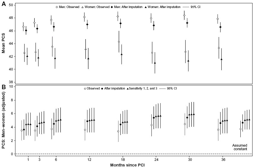
Looking at the course of MCS for men and women separately, we found that women’s scores were initially nearly six points lower than men, and they reported a larger increase over time compared to men. Thus, the courses did not change after imputation; only the level was different (Figure 4A).
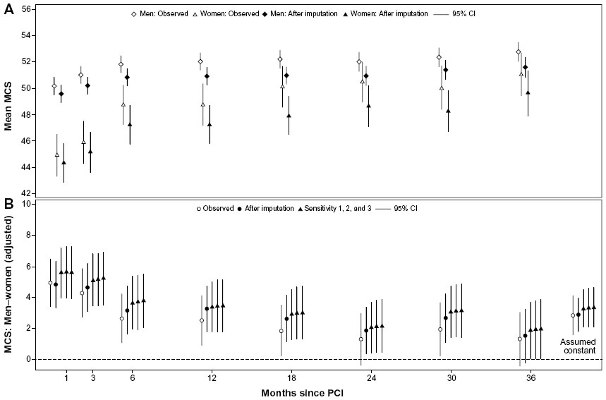 | Figure 4 Sex-stratified unadjusted MCS mean scores: observed and imputation A (A); adjusted differences in MCS: observed, imputation A, and sensitivity analysis (B). |
Using the different datasets (observed, imputed [Scheme A], and the three scenarios of sensitivity analysis [1–3]) in the analytic model of sex differences showed that they were robust to both imputation and in the scenarios of deviations from MAR and comfortably within each other’s confidence intervals. The estimates labeled “assumed constant” are mean sex difference if no time dependence was present (Figure 4B).
Discussion
We have illustrated that MI is a feasible method to try to deal with bias due to missing data in longitudinal studies. In short, we progressed as follows: First, we gained insight in which factors were related to missing data in the relevant variables as well as related to attrition and nonresponse. Second, we obtained additional data (on TPG and date of death) in order to make the assumption of MAR more plausible. Then we specified a regression model for each variable with missing data. The model should resemble how the variable was related to the other variables and support the MAR assumption. The final two steps, generating the imputations and the analysis of the data, required only minimal extra programming compared to a standard statistical analysis. The results based on the imputations are only valid if the data were MAR, and we had specified appropriate imputation models. As these assumptions cannot be validated, we supplemented the analyses by sensitivity analyses based on scenarios with realistic deviations from MAR. The size and direction of these deviations must depend on the specific context, and in this paper, we present only a few variants, while many others are possible. It should be noted that the computations were somewhat time-consuming, for example, with m=100, generating the imputed dataset (one variant) lasted from 1 hour 34 minutes on a personal computer (Windows 7, 64 bit, Intel I7 processor Dual Core 2.4 GHz, 8 GB RAM) to 3 hours 27 minutes on a MacBook (OS10.7.4 Lion, 64 bit, Intel Core 2 duo 2.4 GHz, 4 GB RAM). This time can of course depend on the computer and be further reduced by the use of parallel computing. Since the imputations are generated only once, this could be done overnight or during weekends.
Previous studies have used available SF-12 items in imputations but only in cross-sectional settings, among respondents and with limited use of auxiliary information.31,32 Since we chose to impute the two component summaries from SF-12, and not all 12 items, we experienced some information loss where a single missing item resulted in a missing component summary and information from the non-missing items were not used. On the other hand, our imputation model would have been increased with 80 additional equations, if each item at each time point should have been imputed and thus prone to small strata as the single items are categorical.
Few previous studies have used MIs to deal with missing SF-12 (or SF-36) data in a cohort with repeated follow-ups. We found one small study that used weighing to adjust for sampling bias.33 In patients with heart disease, Weintraub et al used MI to impute intermittent missing scores in the SAQ and SF-36 in a study with repeated measurements, following the same time pattern as our study.34 Their imputation strategy was to impute intermitting missing only, and not nonrespondents or patients who dropped out. Since we found important differences between respondents compared to nonrespondents or patients who dropped out, we found it important to include these patients in the imputation models as well.
Imputation has previously been used in longitudinal studies. In a recent review, Enders suggested using MI methods instead of complete case analysis and that the choice of MI method should depend on context and assumptions behind the mechanisms of missing data.35 Fielding et al compared different single imputation methods with MI methods and found that MI was superior to single imputation in quality of life data.29 In a longitudinal simulation study, Twisk and de Vente compared different imputation approaches including MI.36 They recommended MI or longitudinal single imputation that led to similar different point estimates after imputation; however, MI had more valid variability compared to longitudinal single imputation.
We have identified a few simulation studies with a longitudinal design that took into account that deaths occurred during follow-up.16–18 Most other studies used MI only in patients who took part in the complete study course; however, some used MI to impute time to death as an outcome.37 Other studies have used the strategy to replace dead persons’ HRQOL scores with 0.5,6 The latter option would underestimate the mean scores in the population still alive, as patients who die during follow-up are contributing to the mean with the value 0.
The very similar results in our study after the different practical approaches of dealing with death in the imputation models may be related to the low number of incident deaths in the follow-up period. In similar situations with few incident deaths during follow-up, it seems safe to use the simplest applicable method, imputing all missing data including those at the first planned questionnaire after death and afterward recoding the latter to missing. However, in other populations with higher mortality rates, different approaches should be applied to evaluate the importance of the method of choice. If the number of dead patients is large, an indicator of death is desirable. How to handle death when using the following measurements in the equations is thus still unknown, and requires further studies in settings with higher mortality than in the present study.
In this paper, we have reported the observed data, five different variants of handling death, and three different scenarios of deviations from MAR for illustrative and pedagogical purposes. In the paper reporting the results,20 we reported the imputed (Scheme A) data only, along with sensitivity analyses. We did not wish to compare observed data with the imputed data when we reported the results, as we were convinced that analyses based on the observed data were wrong. Instead, we reported the imputation models, so that the reader can assess these models, similar to the reporting of how a model of confounder adjustment is defined in a traditional epidemiological study.
Problems with missing data, attrition, and nonparticipation in longitudinal studies have previously, to a large extent, been ignored. MI is implemented in most standard software packages available to epidemiologists. MI is a relevant choice of method, if the assumption of MAR can be made plausible and should be considered in all longitudinal studies.
Ethics statement
The Danish Data Protection Agency approved the study, Ref # 2007-41-0991.
According to Danish law, approval by the Ethics Committee and written informed consent are not required in questionnaire-based and register-based projects.
Additional information is available at The National Committee on Health Research Ethics’ webpage in the “Act on Research Ethics Review of Health Research Projects” § 14.2, available from: http://www.cvk.sum.dk/English/actonabiomedicalresearch.aspx.
The questionnaire data were collected with an identification number, to enable combination with register-based health data, in accordance with the approval from The Danish Data Protection Agency.
Disclosure
The authors report no conflicts of interest in this work.
References
Deeg DJ, van Tilburg T, Smit JH, de Leeuw ED. Attrition in the longitudinal aging study Amsterdam. The effect of differential inclusion in side studies. J Clin Epidemiol. 2002;55(4):319–328. | |
Brilleman SL, Pachana NA, Dobson AJ. The impact of attrition on the representativeness of cohort studies of older people. BMC Med Res Methodol. 2010;10:71. | |
Chatfield MD, Brayne CE, Matthews FE. A systematic literature review of attrition between waves in longitudinal studies in the elderly shows a consistent pattern of dropout between differing studies. J Clin Epidemiol. 2005;58(1):13–19. | |
Diehr P, Patrick DL. Trajectories of health for older adults over time: accounting fully for death. Ann Intern Med. 2003;139(5 pt 2):416–420. | |
Diehr P, Patrick DL, Spertus J, Kiefe CI, McDonell M, Fihn SD. Transforming self-rated health and the SF-36 scales to include death and improve interpretability. Med Care. 2001;39(7):670–680. | |
Ratcliffe J, Young T, Longworth L, Buxton M. An assessment of the impact of informative dropout and nonresponse in measuring health-related quality of life using the EuroQol (EQ-5D) descriptive system. Value Health. 2005;8(1):53–58. | |
Bowe S, Young AF, Sibbritt D, Furuya H. Transforming the SF-36 to account for death in longitudinal studies with three-year follow-up. Med Care. 2006;44(10):956–959. | |
Diehr P, Patrick DL, McDonell MB, Fihn SD. Accounting for deaths in longitudinal studies using the SF-36: the performance of the physical component scale of the short form 36-item health survey and the PCTD. Med Care. 2003;41(9):1065–1073. | |
Rothman KJ, Greenland S, Lash TL. Modern Epidemiology. 3rd ed. Philadelphia: Lippincott Williams & Wilkins; 2008. | |
Verbeke G. Linear Mixed Models in Practice: a SAS-Oriented Approach. New York: Springer; 1997. | |
Twisk JWR. Applied Longitudinal Data Analysis for Epidemiology: a Practical Guide 1962. New York: Cambridge University Press; 2003. | |
Rubin D. Multiple Imputation for Nonresponse in Surveys. New York: Wiley; 1987. | |
Sterne JA, White IR, Carlin JB, et al. Multiple imputation for missing data in epidemiological and clinical research: potential and pitfalls. BMJ. 2009;338:b2393. | |
White IR, Royston P, Wood AM. Multiple imputation using chained equations: issues and guidance for practice. Stat Med. 2011;30(4):377–399. | |
Carpenter J, Bartlett J, Kenward M. Missingdata.org.uk. 2012. Available from: http://www.missingdata.org.uk/. | |
Kurland BF, Johnson LL, Egleston BL, Diehr PH. Longitudinal data with follow-up truncated by death: match the analysis method to research aims. Stat Sci. 2009;24(2):211. | |
Harel O, Hofer SM, Hoffman L, Pedersen NL, Johansson B. Population inference with mortality and attrition in longitudinal studies on aging: a two-stage multiple imputation method. Exp Aging Res. 2007;33(2):187–203. | |
Ning Y, McAvay G, Chaudhry SI, Arnold AM, Allore HG. Results differ by applying distinctive multiple imputation approaches on the longitudinal cardiovascular health study data. Exp Aging Res. 2013;39(1):27–43. | |
Ware JE Jr, Sherbourne CD. The MOS 36-item short-form health survey (SF-36). I. Conceptual framework and item selection. Med Care. 1992;30(6):473–483. | |
Biering K, Frydenberg M, Hjollund N. Self reported health following percutaneous coronary intervention (PCI). Results from a cohort followed for 3 years with multiple measurements. Clin Epidemiol. 2014. Clin Epidemiol. 2014;(6):441–449. | |
Spertus JA, Winder JA, Dewhurst TA, et al. Development and evaluation of the Seattle Angina Questionnaire: a new functional status measure for coronary artery disease. J Am Coll Cardiol. 1995;25(2):333–341. | |
UNESCO. International Standard Classification of Education 1997. Paris: UNESCO; 1998. | |
Pedersen CB. The Danish civil registration system. Scand J Public Health. 2011;39(7 suppl):22–25. | |
Charlson ME, Pompei P, Ales KL, MacKenzie CR. A new method of classifying prognostic comorbidity in longitudinal studies: development and validation. J Chronic Dis. 1987;40(5):373–383. | |
Andersen TF, Madsen M, Jorgensen J, Mellemkjoer L, Olsen JH. The Danish national hospital register. A valuable source of data for modern health sciences. Dan Med Bull. 1999;46(3):263–268. | |
Schmidt M, Maeng M, Jakobsen CJ, et al. Existing data sources for clinical epidemiology: The Western Denmark heart registry. Clin Epidemiol. 2010;2:137–144. | |
Hjollund NH, Larsen FB, Andersen JH. Register-based follow-up of social benefits and other transfer payments: accuracy and degree of completeness in a Danish interdepartmental administrative database compared with a population-based survey. Scand J Public Health. 2007;35(5):497–502. | |
Donders AR, van der Heijden GJ, Stijnen T, Moons KG. Review: a gentle introduction to imputation of missing values. J Clin Epidemiol. 2006;59(10):1087–1091. | |
Fielding S, Fayers P, Ramsay C. Predicting missing quality of life data that were later recovered: an empirical comparison of approaches. Clin Trials. 2010;7(4):333–342. | |
Rubin D. Causal inference through potential outcomes and principal stratification: application to studies with “censoring” due to death. Stat Sci. 2006;21(3):299–309. | |
Liu H, Hays RD, Adams JL, et al. Imputation of SF-12 health scores for respondents with partially missing data. Health Serv Res. 2005;40(3):905–921. | |
Perneger TV, Burnand B. A simple imputation algorithm reduced missing data in SF-12 health surveys. J Clin Epidemiol. 2005;58(2):142–149. | |
Rubenach S, Shadbolt B, McCallum J, Nakamura T. Assessing health-related quality of life following myocardial infarction: is the SF-12 useful? J Clin Epidemiol. 2002;55(3):306–309. | |
Weintraub WS, Spertus JA, Kolm P, et al; COURAGE Trial Research Group. Effect of PCI on quality of life in patients with stable coronary disease. N Engl J Med. 2008;359(7):677–687. | |
Enders CK. Analyzing longitudinal data with missing values. Rehabil Psychol. 2011;56(4):267–288. | |
Twisk J, de Vente W. Attrition in longitudinal studies. How to deal with missing data. J Clin Epidemiol. 2002;55(4):329–337. | |
Youk AO, Stone RA, Marsh GM. A method for imputing missing data in longitudinal studies. Ann Epidemiol. 2004;14(5):354–361. |
Supplementary materials
 | Table S1 Multiple imputation |
Analysis of physical component summary
 | Figure S1 Samples of nine patient-observed data (A) and three different patients observed and imputed data (B–D). |
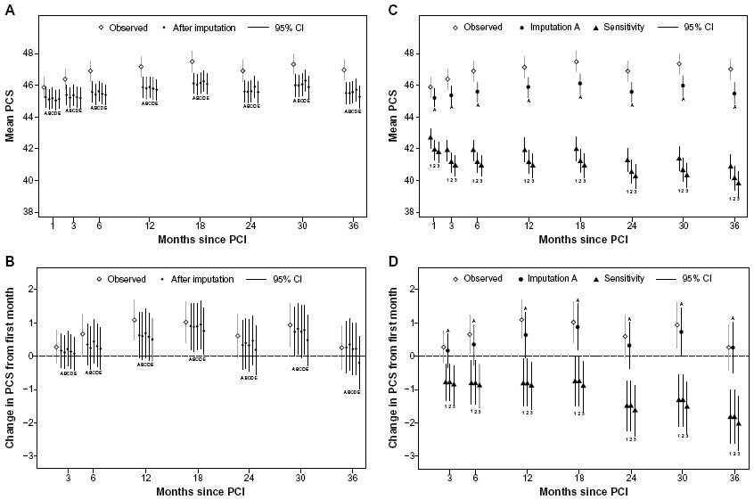 | Figure S2 Mean scores and mean changes of PCS with observed data, variations of approaches related to dead (A and B), and sensitivity analysis (C and D). |
 | Figure S3 Sex differences unadjusted PCS mean scores: observed and imputation A (A); adjusted differences in PCS: observed, imputation A, and sensitivity analysis (B). |
 © 2015 The Author(s). This work is published and licensed by Dove Medical Press Limited. The
full terms of this license are available at https://www.dovepress.com/terms
and incorporate the Creative Commons Attribution
- Non Commercial (unported, 3.0) License.
By accessing the work you hereby accept the Terms. Non-commercial uses of the work are permitted
without any further permission from Dove Medical Press Limited, provided the work is properly
attributed. For permission for commercial use of this work, please see paragraphs 4.2 and 5 of our Terms.
© 2015 The Author(s). This work is published and licensed by Dove Medical Press Limited. The
full terms of this license are available at https://www.dovepress.com/terms
and incorporate the Creative Commons Attribution
- Non Commercial (unported, 3.0) License.
By accessing the work you hereby accept the Terms. Non-commercial uses of the work are permitted
without any further permission from Dove Medical Press Limited, provided the work is properly
attributed. For permission for commercial use of this work, please see paragraphs 4.2 and 5 of our Terms.