The Mechanical Impedance of the Human Skull via Direct Bone Conduction Implants

Introduction

Background

The mechanical point impedance Z is a structure’s resistance to vibrations at a certain point of interest and is defined by the complex quotient of magnitude and phase between applied force in Newtons and the resulting velocity in meters per second according to

1

Knowledge of the mechanical point impedance has played an important role in the technical development of many disciplines, including automotive engineering, civil and acoustic engineering, as well as in biomedical applications. The “mechanical point impedance of the human head”, with or without direct access to the skull bone, has been of fundamental importance in order to understand and develop bone conduction hearing devices especially when having a direct attachment to the skull bone where we use the shorter term “skull impedance”.

In all these bone conduction systems, the transducer (synonymous with vibrator or speaker) interacts mechanically with the mechanical impedance of the load, which depending on the type of device, is the human head with or without skin penetration. Therefore, this impedance will have a direct influence, not only on the performance of the bone conduction devices but also on how to develop artificial loads needed for objective measurements of the frequency responses needed for quality control of such devices.

Before going into the interpretation of the mechanical impedance of the human head per se, we provide a short summary of some applications that rely on the mechanical impedance of the human head as load.

Bone Conduction Hearing Devices

Bone conduction hearing devices are increasingly used in patients with conductive disorders, typically those with mechanical impairments in the transmission of sound from the outer to the inner ear. Today, such devices are commercially available from different manufacturers and in different forms for both percutaneous (direct bone drive) and transcutaneous (over skin drive) devices; for a review see Reinfeldt et al 2015.¹ Figure 1 illustrates the two currently available percutaneous systems (Baha^® from Cochlear, Mölnlycke, Sweden; and Ponto^® from Oticon Medical, Askim, Sweden) using percutaneous osseointegrated titanium implants. These are by far the most used direct bone drive systems, with more than 300,000 patients operated worldwide to date (Håkansson et al 2019²).

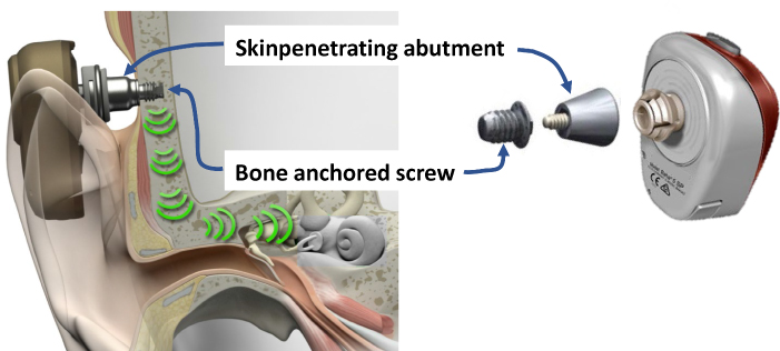Figure 1 The Ponto® system (left) snapping to the outside and the Baha® system (right) snapping to the inside of the skin penetrating abutments that are attached to similar osseointegrated bone-anchored screws.

Other types of bone conduction devices are available; these are named as “active transcutaneous” devices (or “direct bone drive devices with implanted transducer”) and “passive transcutaneous” devices (or “over skin drive devices with implanted retention magnet”), both of which leave the skin intact; for a review, see Reinfeldt et al 2015¹ and Håkansson et al 2019.² Furthermore, bone conduction transducers are also used in consumer products, with the intention of being applied over intact skin, such as in headsets, speech training systems, and for diagnoses of hearing and vertigo (Fredén Jansson et al 2015,³ Håkansson et al 2018⁴).

Artificial Mastoids and Skull Simulators

To be able to measure the mechanical output of bone conduction devices, it is necessary to have adequate mechanical loading of these devices and a sensor that measures the mechanical output objectively. Such artificial loads have been developed and include artificial mastoids representing the load of the skin-covered skull, and skull simulators representing the load seen by direct bone drive devices (percutaneous or active transcutaneous devices). These artificial loads are not only very important accessories for objective measurements of the mechanical output in hearing devices but also for calibration of bone conduction transducers for hearing and vestibular diagnostics. Diagnostic transducers for bone conduction hearing testing (such as the B81) and for vestibular testing (such as B250 as proposed by Håkansson et al 2018⁴) are calibrated using an artificial mastoid B&K4930 from Bruel & Kjaer, having an intact skin pad as load. For direct bone drive devices, a skull simulator is needed that in some way simulates the skull impedance. The first design (Figure 2, left) was invented by Håkansson et al 1989⁵ and remains the current technical standard. This design is based on the finding that the mechanical impedance of percutaneous bone-anchored implants in the human skulls (the skull impedance) is much higher than the mechanical output impedance of the transducer itself, which means that they can be regarded as a constant force source. Thus, the quite complex mechanic impedance of the human skull can in this artificial application be represented by a more simple structure such as a pure mass. This mass load (m) should then be at least three times larger than the mass of the transducer for the transducer to still be considered as a constant force source. The force excitation can then be indirectly measured by an accelerometer (F=m*A according to the second law by Newton) which own mass is included in that mass load (m), see patent SE 8502411 with English abstract SE452238B.⁶ It should be noted that only the stimulating force will be relevantly measured by these devices, but not the resulting acceleration. This is good enough for most purposes, but this method will not be relevant for feedback loop measurements which still needs to be investigated in vivo. Currently, two brands of skull simulators are commercially available for percutaneous direct bone drive devices, both of which use the same design principle. These are the SKS-10 from Interacoustics A/S, Denmark (see Figure 2, middle), and the Verifit^® Skull Simulator VA300 from Audioscan, Canada (see Figure 2, right).

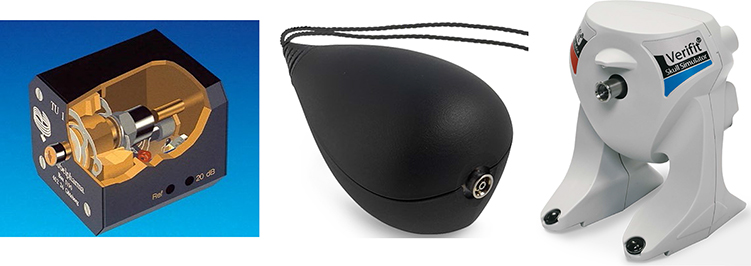Figure 2 Skull simulators as originally invented (left) and commercialized version by Interacoustics (middle) and Audioscan (right).

The Concept of Mechanical Impedance – Skull Impedance

Generally, a mechanical point impedance as expressed in Eq. 1 has a magnitude in Ns/m (or mechanical Ohms) and a phase in degrees where the latter can be anything between +90 degrees for a pure mass and −90 degrees for a pure spring. A pure mass is defined by its mass in Ns²/m (or kg), whereas a spring is defined by its compliance in m/N which is reciprocal to stiffness. A real system has a point impedance that is neither perfectly mass- nor stiffness-controlled due to damping Ns/m, but the phase will always be within ± 90 degrees if the force and the velocity are measured in the same point. Normally all free systems are mass-controlled if the frequencies are sufficiently low and a transition towards stiffness-controlled impedance will take place after a first forced resonance, often called anti-resonance. This anti-resonance is created when the mass and the local attachment compliance of the system interact so that the motions in the attachment point are heavily reduced due to a peak in the point impedance. At higher frequencies, the point impedance will be mainly characterized by the compliance and therefore the impedance will be defined as stiffness-controlled. Further transitions between stiffness and mass-controlled regions may take place at higher frequencies.

Regarding the mechanical impedance of the human skull, one should note that this first anti-resonance is a forced mode phenomenon that appears because of the driving point attachment to the skull. This should not be confused with the free resonances of the skull, which show up at higher frequencies typically from 800 Hz and upwards (Békésy 1960,⁷ Håkansson et al 1994⁸), and which exist when the skull is not affected by any external attachment. Even though the free skull resonances can be detected in the mechanical point impedance data using some specific signal processing methods, they will not normally have any significant importance in terms of the magnitude and phase of the mechanical point impedance, as they will be determined by the bony structures beyond the local attachment point of the skull.

For the proper design of percutaneous bone conduction devices and skull simulators, which is the focus of this paper, the mechanical impedance of the human skull with a direct attachment to the skull bone (the skull impedance) needs to be known. Although this has been investigated in several studies, these studies were made on an older version of the implant system and have shortcomings, for example, have been conducted on a low number of subjects as will be discussed below.

After the first patients were operated on and received implants for attaching a bone anchored hearing aid in 1977, a first mechanical impedance study was presented by Tjellström et al 1980,⁹ who measured eight subjects at some audiometric frequencies by manual readings of amplitude and phase. That study revealed that there is a compliant characteristic of the mechanical impedance above 250 Hz, but also that there was an increasing damping behavior below 250 Hz. As the frequency resolution was poor and the manual readout had low amplitude resolution, Håkansson et al 1986¹⁰ conducted a more detailed study on seven subjects with percutaneous bone-anchored implants. Since then, no studies (as far as the authors are aware) have investigated the mechanical impedance of such implants on living subjects.

In summary, the results from Håkansson’s 1986 study showed that the mechanical impedance at the osseointegrated percutaneous implants had an anti-resonance at approximately 145 Hz and that the impedance magnitude was 10–30 dB higher than the impedance of intact skin over the skull. These results were then used to design a transducer optimized for bone-anchored hearing aids with a single housing design (Håkansson et al 1985¹¹). These results were also used to develop a skull simulator for quality assurance and verifying fitting of percutaneous devices (Håkansson et al 1989⁵).

However, the Håkansson’s 1986 study needs to be updated, for several reasons. First, it was conducted on a limited number of patients, which does not allow for analyses of gender, age, syndromes, and major ear surgeries. Secondly, in those measurements, the attachment was made by manually pressing the impedance head towards the implant, with hands on both sides of the head, which creates additional variability regarding measurement direction and static force. Third, a coupling via a metallic tip (~1 mm²) was used, representing the metallic bayonet coupling used in the early designs, which is not the same as seen by today’s percutaneous snap coupling devices. Fourth, a random noise excitation method was used, which is fast but results in a lower SNR than with swept sine. Finally, the mass compensation was made by a physical electrical network subtraction, which is less accurate than a pure mass parametric mathematical subtraction from the apparent mass function (force/acceleration).

Given that the trend is still towards treating patients with direct drive bone conduction devices, and in view of the lack of detailed studies of the skull impedance via such implants, we decided to re-measure the mechanical impedance on a greater number of patients using the latest versions of percutaneous snap coupling implants.

Aim of Study

The main aim of this study is to measure the mechanical skull impedance of percutaneous implants on a larger group of subjects treated with bone anchored hearing devices. The results will be analyzed regarding age, gender, ear surgeries, and malformations that could potentially affect the impedance.

A secondary aim is to analyze these experimental results, by modelling of the mechanical impedance and the transducer, in order to investigate if the median impedance has any influence on the performance of bone anchored hearing devices, either fitted on aided patients or when measured on a skull simulator.

Methods and Materials

Measurement Setup

The setup for the present mechanical point impedance measurements is based on an impedance head from Brüel & Kjær (B&K 8001) driven by a BEST transducer (Fredén Jansson et al 2015³) with a resonance frequency boost at 250 Hz. The impedance head has two piezoelectric crystals arranged so that one is sensitive to the force (F) and one is sensitive to the acceleration (A) at the attachment point. Corresponding voltage signals V_F and V_A are available at connector ports on the side of the impedance head. From the quotient V_F/V_A the mechanical impedance can be calculated, as described below. The BEST transducer, which provides the mechanical vibrations, was screw-attached to the backside of the impedance head, whereas the snap adaptors A (Baha^®) or B (Ponto^®) were attached to the front side of the impedance head, as illustrated in Figure 3. These snap couplings firmly attach the transducer in the sound processor to the bone-anchored abutments (also shown in Figure 1) along the same axis as the implant. The abutments are either of the traditional Baha design that fits to both snaps A and B, or the newer Baha specific abutment BI 300, which only fits to snap A. The osseointegrated screws have either a diameter of 3.75 mm or, in a later design, 4 mm but we have assumed that this difference will be of negligible influence for the mechanical impedance.

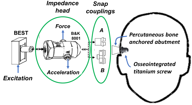Figure 3 Mechanical point impedance set-up comprising an excitation transducer (BEST) and an impedance head (B&K 8001) and two different snap couplings A and B, where A snaps into the inside of the abutment and B snaps over the outside of the abutment. The osseointegrated implant comprises an osseointegrated titanium screw and a skin penetrating titanium abutment firmly attached to each other by an internal screw not shown in the figure.

This is a joint research study between the Universities in Gothenburg, Sweden, and Edmonton, Canada. Some of the measuring equipment was slightly different at the two sites, but that is not assumed to affect the measurements. In Gothenburg, all signal acquisition and processing were based on an Agilent 35670 signal analyzer that also could directly drive the BEST transducer during the excitation. The analyzer simultaneously measures acceleration and force signals produced by the impedance head after first passing charge amplifiers (B&K 2635 and B&K 2651). In Edmonton, a PC-based LabVIEW program was developed, and a separate power amplifier was used to efficiently drive the transducer. Charge amplifiers were used before the signals were fed to the USB data acquisition card in the laptop.

All calibration procedures were the same in Edmonton and Gothenburg. Prior to all measurements the measured complex function V_F/V_A was calibrated against a known pure mass of m=50 g, theoretically giving a frequency independent magnitude of 0.05 kg and zero phase (F=m*A). The calibration factor “α” was extracted at 1 kHz which scales the signals to obtain the correct magnitude of F/A. This correction of the measured V_F/V_A response was made in each patient in the post-processing by a multiplication of the calibration constant “α”, as shown in Eq. 2. Subsequently, the mass m₀ above the force gauge of the B&K 8001, which should not be included in the skull impedance, was mathematically cancelled by subtraction.

2

Finally, a multiplication by jω (j is the complex constant and ω=2πf is the angular frequency) was made to transform acceleration to velocity in order to achieve the mechanical point impedance Z of the skull.

All measurements were performed using a swept sine comprising 401 logarithmically spaced frequencies from 100 Hz to 10 kHz covering frequencies of interest for bone conduction hearing implants. The force excitation level was determined based on that the signal level should be sufficiently high to exceed the noise level for most frequencies, but low enough not to annoy the patient. From normal hearing level data, as determined by Carlsson et al 1995,¹² it was decided that a rms level of 200 µN corresponding to a hearing level of 45 dB HL at 1 kHz was sufficient and did not annoy the patient. Even if the dB HL seems to be relatively low, this excitation level is much higher than used in the previous wideband excitation¹⁰ as here all energy is concentrated to one frequency at a time, whereas in a wide band noise measurement it is spread out over the whole frequency range under investigation and averaging is needed to reduce uncorrelated noise. Unwrapping of the phase response was necessary above 200 Hz, due to fluctuations temporally passing below −90 degrees, which was made manually afterwards by subtracting 360 degrees on such occasions.

Modeling of the Mechanical Impedance

The most interesting question is if the difference in the mechanical impedances will affect the output of bone conduction hearing implants. In order to study this, simulations based on models of both a mechanical skull impedance and the transducer are needed. In the study by Håkansson et al 1986,¹⁰ the mechanical skull impedance was modeled by an electro-mechanical analogy based on mass, stiffness, and damping parameters extracted from the median mechanical skull impedance which also is adapted here but with a simplified topology adapted to present result, see the Discussion section. For the simulations, the electronic work bench program Multisim ver. 14.1 from National Instruments is used where inductors (Henry, H) correspond to masses (kg); capacitors (Farad, F) correspond to compliances (m/N); resistors (Ohm, Ω) correspond to dampers (Ns/m); voltage (V) corresponds to force (N); and current (A) corresponds to velocity (m/s). For more detailed background to electro-mechanical analogies, see Baranek and Mellow 2012.¹³

Patients

A total of 45 subjects (20 male, 25 female) participated, who were recruited as a consecutive prospective case series, and their average age when tested was 55.4 yrs (range 18–80 yrs), see Table 1. Seven patients were tested in Gothenburg, Sweden and the remaining 38 patients were tested in Edmonton, Canada. Twenty-six patients were considered to have normal skull anatomy, 15 had gone through mastoidectomy on the implanted side when tested, and four patients had different syndromes (Down syndrome, Waardenburg syndrome, Treacher Collins syndrome, and Charge syndrome). Most patients had a traditional abutment that was compatible with both brands of percutaneous devices (Figure 1), whereas some could only use devices from one of the manufacturers (the one with snap A).

The results were analyzed on a group level using medians and standard deviations. For subgroup comparisons, the amplitudes and phases were statistically analyzed using the t-Test for “Two sample for means” where a probability value of p < 0.05 was considered for rejecting the null hypothesis, ie that there is a significant difference between subgroups.

The study was conducted in accordance with the principles stated in the Declaration of Helsinki where applicable (ethic approval no: Pro 0020939), and the test subjects gave their informed consent to participate in the study after being informed. This research was approved by Chalmers University of Technology, Gothenburg, Sweden and University of Alberta, Edmonton, Canada.

Participation in the study was voluntary and no remuneration was given to the test subjects.

Results

All Subjects

Figure 4 shows the magnitude and phase of the mechanical point impedance of all 45 subjects, while the median values are shown by the thick black lines. Medians were preferred instead of averages because they discard extreme and possible outlier values, but the differences between average and median values were actually very small; see Table 2. Percentiles, averages, and standard deviations (STD) are shown for the most common audiometric frequencies. As seen in Table 2, median and average values (bold) are very close to each other for frequencies above the low-frequency anti-resonance.

Table 1 Forty-Five Patients Investigated at Two Sites

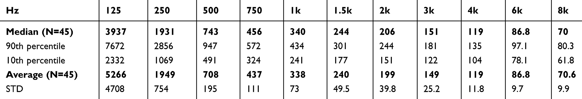Table 2 Magnitude Values of the Mechanical Impedance of the Skull Z in Ns/m

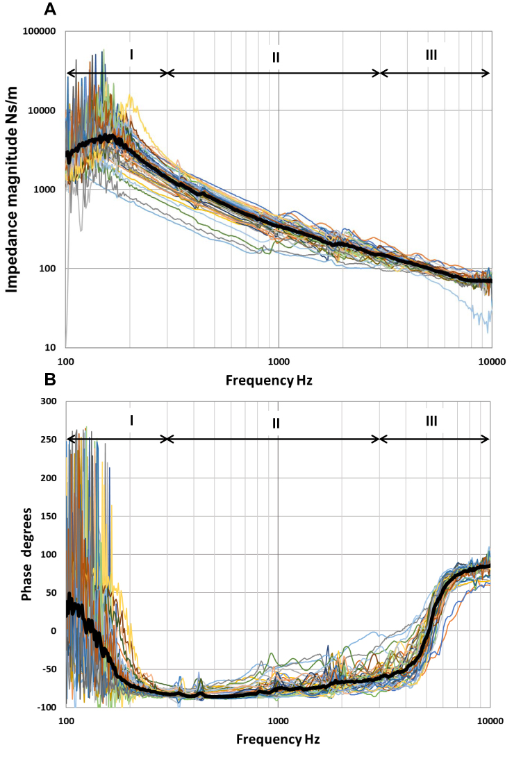Figure 4 Individual magnitude (A) and phase (B) of the skull impedance of all the 45 subjects tested. The median value is presented by the thick black line. The impedances are divided in the analysis into a low-frequency region (I), a mid-frequency region (II) and a high-frequency region (III) depending on the phase characteristics.

As it was found that none of the variables analyzed (age, gender, surgeries, syndromes, couplings, and sites) will influence the device performance in the clinical application significantly (see simulations in the Discussion), the results from all subjects are pooled together to identify characteristic parameters from the overall median results in what follows.

In a more detailed analysis, the overall group results are divided into three frequency regions I, II and III, where Region I is covering the low frequencies (100–300 Hz), Region II covers the mid-frequency range (300–3k Hz), and Region III covers the high frequencies (3–10 kHz). These regions are defined based on changes in the impedance behavior, as most obviously seen when looking into the phase responses in Figure 4. Thus, in Region I the mechanical median impedance phase has a transition from mass controlled to stiffness controlled (from positive to negative phase); in Region II the impedance is rather stable and is stiffness-controlled (negative phase); and in Region III the impedance has a transition from stiffness- back to mass-controlled again (from negative to positive phase).

Region I: Low Frequencies 100–300 Hz

In this region, the division of the two measured responses (F/A) become a bit noisy when doing the sweep over all frequencies in one session. The noise at low frequencies is mainly dependent on a low acceleration (A) response as the impedance magnitude is relatively high in this frequency region due to the dominant anti-resonance. Also, a lower force output (F) of the stimulating transducer can contribute to the noise at the lowest frequencies below the transducer resonance frequency at 250 Hz. The magnitude and phase responses for the median for this frequency range are shown in Figure 5, together with a multiple-order polynomial model (Excel) fitted to the data giving trend lines in order to more systematically estimate the characteristic parameters.

Figure 5 Median magnitude (A) and phase (B) of the skull impedance in the low-frequency region 100–300 Hz of all the 45 subjects tested. The 95% confidence interval is shown as by its max and min values. Trend lines were fitted to both the magnitude and phase response from which parameters were extracted.

Combining information from the magnitude and the phase response, it can be stated that the skull impedance is mainly mass-controlled below the anti-resonance (increasing magnitude and positive phase) and that it is stiffness-controlled above the anti-resonance (decreasing magnitude and negative phase). Using the trend lines, the maximum magnitude of the anti-resonance was found to be Z_max=4527 Ns/m at an anti-resonance frequency of f_r=151 Hz. At 100 Hz the total apparent mass (F/A) was found to be 4.3 kg, but the mass reduces to M=2.5 kg if the damping R is taken into account according to Z= jωM+R (the phase at 100 Hz is 36 degrees), where ω is the angular frequency, j the complex constant, and R represents the damping of the real mass M involved. This reduction of the mass involvement in the skull impedance is probably due to the fact that only the upper part of the skull is transversally moving while supported by the more rigid neck and shoulder in its base, also introducing damping to the motion. This means that the effective moving mass will thus be less than what is normally considered to be the total mass of the human head (4.5–5 kg including down to vertebra C3).

Using Eq. 3, valid for a low damped second-order system, and given that M=2.5 kg, and f_r = 151 Hz, one can calculate that the equivalent compliance involved is C445n m/N.

3

Region II: Medium Frequencies, 300–3k Hz

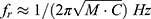
In the mid-frequency region, the mechanical impedance of the skull is clearly stiffness controlled with a rather pure compliance, as the magnitude decreases by −19.2 dB for the full decade in Figure 6 (ideally for pure compliance and no damping, the magnitude should decrease by −20 dB/decade). Obviously, the damping involved in this frequency region is rather small as the phase is relatively close to −90 degrees (starting at lower frequencies around −85 and rising to −60 degrees near 3000 Hz where it is already affected by the mass at highest frequencies). Considering that some damping R is involved using the model Z=R+1/(jωC), the compliances C can be calculated from the trendline and found to be 438n, 473n, 447n m/N at 500, 1k and 2k Hz, respectively. As the corresponding average value is 452n Nm/s, which is very near the value calculated from the low-frequency anti-resonance model in Region I (445n m/N), we conclude that the mid-frequency compliance can be estimated to be C=450n m/N. It should be noted that the major part of this compliance is assumed to originate from the skull bone compliance, but the snap coupling compliance also contributes to some minor extent, see separate coupling measurements for snap A and B.

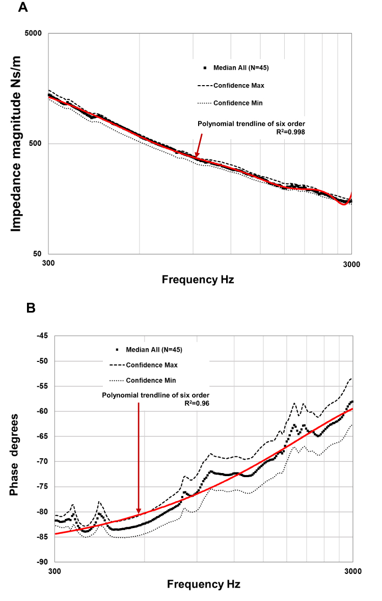Figure 6 Median magnitude (A) and phase (B) of the skull impedance in the medium frequency region 300–3k Hz of all the 45 subjects tested. The 95% confidence interval is shown as by its max and min values. Trend line of a 6th order polynomials (Excel) was fitted from which parameters were extracted.

Region III: High Frequencies 3–10 kHz

For frequencies 3–10 kHz, the mechanical impedance transforms gradually from a stiffness behavior to a mass behavior with some damping, even though this is mainly visible in the phase response approaching positive degrees whereas the magnitude flattens out (Figure 7). The absence of clearly increasing magnitude with frequency might have to do with the fact that the interpretation of the vibration characteristics is more complex and lumped parameters suffer interpretation at high frequencies when the wavelength is in the same range or shorter than the dimensions of the structure.¹⁴ In any case, the measured impedance is what the driving transducer will see. From this trendline, the apparent mass at 10 kHz will be approximately m=1.3 gram. This value seems reasonable as it corresponds approximately to the mass of the titanium implant and some adjacent skull bone.

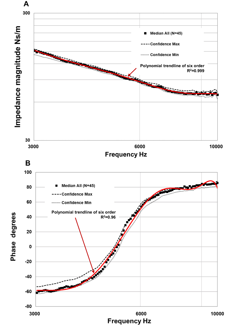Figure 7 Median magnitude (A) and phase (B) of the skull impedance in the high-frequency region 3 to 10 kHz of all the 45 subjects. The 95% confidence interval is shown as by its max and min values. Trend lines of a 6th order polynomials (Excel) was fitted from which parameters were extracted.

Subgroup Analyses

Influence of Gender, Age, Surgeries, and Malformations

There is no statistically significant difference (average p=0.52 over all frequencies) when comparing the mechanical impedances for female (N=25) and male (N=20) patients which is also visually indicated by the medians in Figure 8A. On the other hand, when analyzing subjects younger than 60 years (N=23) against those older than 60 (N=22), one can see a tendency to difference in the compliance, see Figure 8B. However, this difference was not found to be statistically different overall frequencies (p=0.36) but very close to significant for 250–700 Hz (average p= 0.07). The compliance was calculated for the two subgroups at 300 Hz and found to be C_{below 60 yrs} = 390n m/N (−12%) and C_{above 60 yrs}= 480n m/N (+6%) where the percentages are relative to the estimated overall median C=450n m/N. This difference in compliance is most likely the reason that the anti-resonance frequency is slightly higher in the older group than in the younger group, 158 versus 135 Hz. As mentioned, part of this compliance is due to the snap coupling, which should not be patient age-dependent, so the influence of bone compliance in percentage due to age might be even higher.

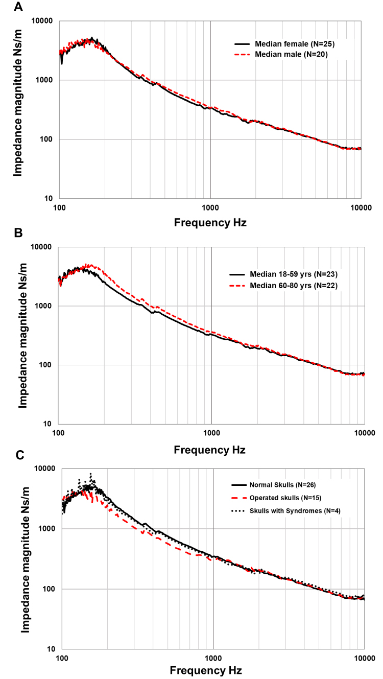Figure 8 Mechanical impedance data pooled for comparing gender (A), age (B) and subjects that has gone thru mastoidectomy and those with syndromic skull structure (C).

For those who have gone through a mastoidectomy (N=15), a softening of the skull compliance was seen by the lower curve in Figure 8C where C_op= 502n m/N is calculated at 300 Hz using magnitude Z=1/(ωC_op). Again, the mean impedance magnitude was found not to be significantly different from those with normal skull anatomy (N=26) over all frequencies (p=0.58) or even just looking at the most affected range 250–300 Hz (p=0.33). Neither did those who had a syndromic skull structure (N=4) show any statistical difference in skull compliance in comparison to normal subjects (p=0.43 overall frequencies and p=0.33 for 250–300 Hz).

Gothenburg versus Edmonton Measurements

A separate comparison was made to confirm that the seven patients measured in Sweden were representative of those 38 patients measured in Canada. As Figure 9 shows, there were significant differences at mid-frequencies with an average p=0.026 for 1000–4500 Hz, where the magnitude is slightly higher among the SWE patients than among the CAN patients. It seems that this difference could, at least partly, be explained by the fact that the SWE patients are older than the CAN patients: 66.0 vs 53.4 yrs (overall average was 55.4) resulting in a stiffer bone (lower compliance = higher impedance magnitude). Figure 9 also shows that the CAN patients have almost identical median as all patients.

Figure 9 Median mechanical impedance magnitude (A) and phase (B) of the patients measured in Sweden and Edmonton, respectively. Besides the subgroup medians also the overall median magnitude as well as the corresponding 90th and the 10th percentiles are shown.

Our conclusion is that there are no systematic differences between the two sites except for a possible a minor influence related to the ages of the patients and, therefore, the impedance data can be pooled together, as was done in the present overall analysis.

Different Coupling Systems – Snap A and B

The two different coupling systems, snap A and B, were investigated separately by connecting them to a pure mass of approximately 50 gram and measuring the mechanical impedance, for more details see Woelflin 2011.¹⁵ It was found that the impedance behaves as pure mass up to the first anti-resonance, where the compliance of the couplings interacts with the mass forming a relatively undamped peak at around 1.6 kHz. Using Eq. 3, with the resonance frequency and mass value known, the coupling compliance was calculated and found to be C_A= 163n m/N and C_B=187n m/N, respectively. The coupling compliance from these two coupling types was so close in value that they can be modelled by the average value of Cc = 175n m/N. In these measurements, new unused snap couplings were used, and their compliance may gradually become softer, giving a higher C value over time due to wear. This change over time was not investigated and was beyond the scope of this study. However, the influence of a softer and more compliant snap coupling was simulated and discussed in the Discussion section.

Discussion

General discussion of the Results

It was found that the mechanical impedance for the human skull can be described at lower frequencies by a low-frequency anti-resonance, with an approximate maximum magnitude of Z_max≈4500 Ns/m at approximately f_r≈150 Hz. Above this frequency, the impedance magnitude decreases, characterized by a total compliance of approximately C=450n m/N. This compliance is mainly due to the compliance of the skull bone around the implant which is located in the parietal bone approximately 55 mm behind and slightly above the ear canal opening and to a minor extent to the snap coupling compliance.

These results are also in line with those of Håkansson et al 1986,¹⁰ who found that the anti-resonance peak was on the average 145 Hz and that the skull impedance had mass-controlled behaviors below and compliance-controlled behavior above that frequency. In that study, the peak value was estimated to 3800 Ns/m, but in some of the subjects, there were double peaks at these low frequencies, which not was seen in this study. A single peak behavior will probably result in a slightly higher maximum magnitude value (4500 Ns/m), as double peaks will reduce the magnitude between the peaks. The absence of double peaks here may be explained by the fact that we used a firm snap coupling to the implant with an almost perfect axial alignment between the impedance head and the implant. In this way, additional rotational vibration modes were avoided due to misalignment between the impedance head and axis of the implant assumed to create double peaks. The previous study also measured the coupling compliance and found it to be stiffer (lower compliance) than in this study: 110n m/N versus 175n m/N. This may be explained by the fact that, in the previous study, a direct stiff metallic contact in the bayonet connector to implant contact, whereas both snaps A and B use non-metallic materials.

The present results generally show that there was no statistically significant difference between patients with different gender or those with previous major surgery in the temporal region relative to those with normal temporal bones. One minor deviation found, even though not significantly different, was that patients with older ages may have a slightly stiffer or less compliant bone than in those of younger ages. Such hardening of bone tissue is well known and explained by that bone, in general, calcify and harden with age. Another observation that was made in this study is that patients who have undergone a mastoidectomy will have slightly more compliant bone at the implant site, most likely because some stabilizing bone in the temporal region has been removed.

Descriptive Explanation of the Mechanic Impedance of the Human Skull

Over the years many have raised questions about how the mechanical impedance of the skull should be interpreted and if it has any importance for the clinical outcome using bone conduction implants. The clinical outcome will be discussed under the modelling section below but regarding the interpretation Figure 10 provides a simplified proposed description of how the skull moves when subjected to a dynamic force excitation at the implant site for frequencies at and around the anti-resonance.

Figure 10 Illustrations of skull motions proposed for frequencies below, at and above the anti-resonance frequency typically located at 150 Hz.

First, below the anti-resonance, left illustration in Figure 10 shows that the lower part of the skull is relatively immobile as it is connected to the firmer spinal cord, neck and upper shoulder portion. Therefore, the moving effective mass is lower than the total mass of the skull, in this study found to be approximately M=2.5 kg. This rather firm connection to neck and shoulder may explain why there is considerable damping when the skull is moving back and forth at these low frequencies (phase is only 36 degrees at 100 Hz, whereas 90 degrees is expected for a pure mass). Secondly, at the anti-resonance (middle illustration in Figure 10), it is very hard to dynamically move the skull at the attachment point as it has a very high impedance. This is because the compliance in the skull bone interacts with the moving mass on the “other side” of that compliance in such a way that the force of the other sides’ moving mass acts in the opposite direction and thus counteracts the excitation force synchronously. Obviously, the skull portion of the other side of the skull can still move quite heavily at the anti-resonance frequency even if the excitation point of skull hardly can move. Thirdly, for higher frequencies, this mass of the “other side” is decoupled and is hardly moving at all as shown in Figure 10 (right illustration). What is seen here is then just the compliance of the skull bone on some distance around the implant and the snap coupling. At the highest frequencies, only the mass of the implant and mass of the bone very close to the implant is involved, so at these frequencies the impedance will be mainly mass-controlled.

Linearity of the Mechanical Impedance

One fundamental assumption needed for the interpretation of the output of bone conduction implants based on the skull impedances among the patients is that the skull impedance is linear; that it has the same magnitude and phase independent of the stimulation level. The linearity properties of the skull impedance were verified in one of the patients, where the impedance measurements were repeated at several excitation levels and no nonlinear behavior was detected. This has also been confirmed in other studies by Håkansson et al 1986¹⁰ and 1996,¹⁶ who found a linear behavior of the skull impedance for speech hearing levels.

Modeling of the Mechanical Impedance

Here we propose a slightly different and simplified topology of the electro-mechanical model than proposed by Håkansson et al 1986,¹⁰ which is shown in Figure 11 (left). The model magnitude of the impedance is shown in Figure 11 (right panel – black dashed line) together with the measured skull impedance magnitude (right panel – solid line). The parameters and values included are: skull mass M=2.5 H and related damper R=1180 Ω; bone compliance Cs=280 nF; snap coupling compliance Cc=175 nF was extracted as previously explained from the impedance results. The damping of the skull bone, Rs=90 Ω, was determined to give the desired magnitude at 5–7 kHz and the mass Ms=1.3 mH was added to account for the mass of the implant and the adjacent attached bone, which accounts for the mass behavior above 5–7 kHz. It should be noted that the total compliance at low and medium frequencies equals the sum of the skull compliance and the coupling compliance (CCc + Cs) as they are in parallel and Rs is negligible. The difference between the measured median magnitudes in this study and the model magnitudes are small and differ just slightly (by less than 25%, ie 2 dB) in the 2–8 kHz region. Also plotted by red squares in Figure 11 (right) is the average values from Håkansson et al 1986¹⁰ where this deviation was higher above 1 kHz. One reason for this deviation might be that the present snap couplings are much softer (175 nF) than the metallic coupling (110 nF) in the earlier study thus dominating the compliance in this region. These differences in magnitudes for higher frequencies were anyway found to be of negligible clinical importance; see the variability evaluation below.

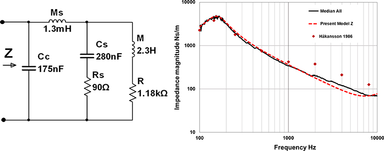Figure 11 Electro-mechanical analogy model of the skull impedance (left) and the median skull impedance magnitudes (right) of all subjects (solid line), the proposed model (dashed line) and the model used by Håkansson et al 1986 (squares).

Influence of Skull Impedance Variability Using Bone Conduction Implants

To study the influence of the skull impedance variability on device performance, we need to simulate how the output force is affected. For such simulations, not only a model of the skull impedance but also a model of the transducer is needed. Using such models one can also evaluate how the mechanical output on a skull simulator differs from the real output on a patient.

To do this evaluation, the bone conduction transducer can be modeled by an electro-mechanical analogy and then connected to a model of the skull impedance, as shown in Figure 12. The transducer model is taken from Håkansson et al 1984,¹⁷ which, with some few modifications, conforms with later designs of bone conduction transducers. Here, the transducer performance is determined by the output force (Fout) divided by the voltage driving the transducer (Vin) when loaded with either a model of the skull impedance or a model of the skull simulator as indicated in the left side of the network in Figure 12.

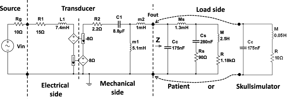Figure 12 Complete electro-mechanical analogy model of a typical transducer connected to either the proposed model of the skull impedance or a model of a skull simulator.

As is shown in Figure 12 the skull simulator has a very different mechanical impedance model than that of the skin penetrated human skull. The skull simulator model is taken from Håkansson et al 1989⁵ and consists of a mass of 50 gram but now also with a small series damper 2.2 Ω (to limit the resonance peak that would otherwise be infinite) and a snap coupling compliance of Cc=175 nF included.

It is apparent from Figure 13, that the transmission function with the skull simulator as load is only slightly affected as compared to when a patient with a skull impedance Z is connected. The most important difference is that the transducer resonance at around 750 Hz is moved slightly upwards by approximately 50 Hz when attached to a skull simulator. This can be important if a fixed electronic damping algorithm is used for the damping of the transducer resonance. There is also some deviation above 8 kHz because the skull impedance is more damped than the coupling having a rather undamped spring compliance at these frequencies. Good agreement in force output response between the real skull impedance and the skull simulator impedance confirms the underlying assumption that the transducer acts an almost constant force source independent of the load impedance.

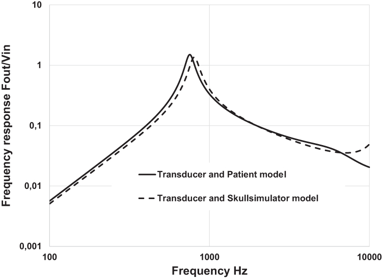Figure 13 Frequency response when the transducer model is attached to the skull impedance model (solid line) and to the skull simulator model (dashed line).

It is now also interesting to know how the variability in the skull impedance affects the frequency response in the individual patients. By connecting the same the transducer model to the model of the load where the parameters are set to represent extreme values of the patient impedances, we can investigate how this variability may affect the in vivo frequency response of these devices. The transducer model is rather robust as electrical and mechanical components are almost the same in all devices, whereas the skull impedance of the patients may vary considerably as shown in Figure 4. In a first simulation session, the transmission function was calculated for the assumed extreme values of Cs assumed to be 140n and 560n m/N, which is +100/-50% of the nominal value 280n m/N. This range of compliances embraces the impedance magnitude variability within the 90^th and the 10^th percentiles up to 3 kHz in the present study as seen in Figure 14A. In Figure 14B, where curves for this simulation are plotted only for 100–3k Hz, it is obvious that the transmission function is hardly affected below 3k Hz (<1 dB) despite that the changes in Cs are substantial.

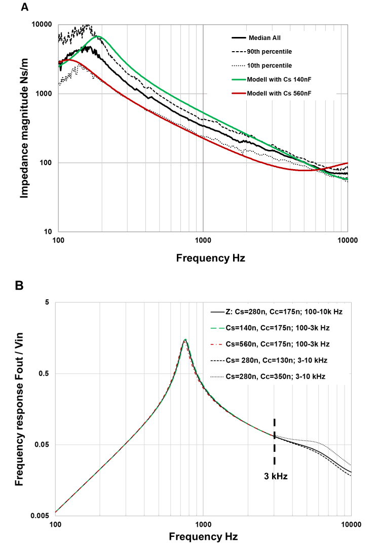Figure 14 Median, 90th and 10th percentiles of the measured skull impedance magnitudes and the modeled skull impedance magnitudes with extreme values of Cs (A). Magnitudes of the simulated frequency response using the electro-mechanical analogy model of the transducer and modelled impedance (B) where besides nominal values of Cs (280nF) and Cc (175nF) also the extreme values of skull compliance Cs and coupling compliance Cc are used. Note that only Cs is varied below 3k Hz and only Cc is varied above 3k Hz.

Above 3k Hz the skull impedance is mainly affected by the snap coupling compliance Cc with some influence from parallel network Ms, Cs and Rs (M and R are decoupled above the anti-resonance at 150 Hz). Therefore, the transmission functions above 3 kHz were calculated for an assumed maximum variability of +100/-25% in Cc; that is, using Cc= 130 nF, 175 nF (nominal) and 350 nF. The reason for using asymmetric values of Cc is that it is very difficult to make the coupling much stiffer than in a new coupling having compliance in the range of 175 nF and that the compliance will become gradually softer over time by wear until it must be replaced. For the simulated stiffer coupling (130 nF), the output decreases only slightly (dashed line), but it will increase more significantly for a softer coupling (350 nF – dotted line). As the nominal compliances of snaps A and B are quite similar (163 versus 187 nF), it can be assumed that in clinical use on patients there is no clinical difference between these two designs. However, it looks like a softer coupling could be beneficial in terms of higher output at high frequencies, although there is an overriding requirement for sufficient retention (so that the device will not fall off accidentally) that requires sufficient snap-in function.

When the different values of coupling compliance Cc (130 nF, 175 nF and 350 nF) are simulated with a skull simulator as load, then a more pronounced effect is seen at higher frequencies, see Figure 15. When the coupling is softer by time, one will see a high-frequency peak growing and coming in from higher frequencies above 10 kHz. Obviously, this change in relation to the coupling compliance is more damped in the real patient and does not have any substantial clinical audiological effect as seen in Figure 14B even though snap coupling replacement might be needed to secure sufficient retention. That said, care should be taken when considering the verification of high-frequency output measured on the skull simulator as this coupling compliance may lead to slight misinterpretations of how to a match target gain in this region (Hodgetts & Scollie, 2017¹⁸).

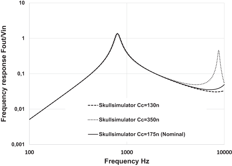Figure 15 The influence of different coupling compliances using the skull simulator as load.

Relevance for Implantable Transducer Solutions

In recent years there has been a development towards implanted transducer solutions; see Reinfeldt et al 2015¹ and Håkansson et al 2019² for a review. In these devices, the transducers are normally attached to the skull bone at a site closer to or within the mastoid cavity of the temporal bone. The mechanical skull impedances at such sites, located close to or within the mastoid, have been investigated in several cadaver studies, see for example Eeg-Olofsson et al 2008.¹⁹ In these studies, the skull impedance was generally found to have a lower bone compliance (higher stiffness) than at the thinner parietal bone where the bone anchored percutaneous devices are attached. Hence, the assumption that the transducer can be regarded as a constant force source when loaded by skull impedance is even more fulfilled here. Therefore, the present commercially available skull simulators can be used to measure the frequency response of also active bone conduction implantable devices with implantable transducers. Practically, this is done by allowing the titanium casing containing the implantable transducer to be attached to the skull simulator using a flat adaptor with a spring lock arrangement; see Håkansson et al 2019.² Also, the variability of the mechanical impedance between patients using these implantable transducers can be assumed to have the same negligible influence on the device performance as shown in this study on percutaneous devices.

For implantable transducers, the coupling to the bone is also more robust than it is for percutaneous devices that presently use either snap A or B. Therefore, one can create the high-frequency boost for implantable transducers, as vaguely indicated in Figure 14B (dotted line), with a Cc greater than 350 nF. Such boosting can be done by a specific mechanic design of the transducer to casing interface, creating a damped resonance peak at, for example, 5 kHz as described by Håkansson et al 2010.²⁰

Conclusions

It was found that the mechanical impedance of the human skull reaches a maximum of 4500 mechanical ohms with an anti-resonance at around 150 Hz, below which frequency it is determined by the mass of the upper part of the skull. For frequencies above the anti-resonance and up to 4–5 kHz, the skull impedance is determined mainly by the total compliance of the skull bone around the implant estimated to be around C=450n m/N including the coupling compliance. At the highest frequencies, above approximately 4–5 kHz, the skull impedance is mainly determined by the local mass of the implant and adjacent bone and some damping.

These results were only slightly, but not significantly, affected by age or if a major ear surgery had been performed. No significant difference was found in relation to gender or skull abnormalities or syndromes.

In simulations using an electro-mechanical analogy model of both the transducer and the skull impedance, it was found that the quite large variability in skull impedance only had a minor effect on the transmission frequency response. Also, compliance differences between snap couplings used by the two commercially available percutaneous bone conduction devices were found to have a negligible influence on the transmission properties.

The results of the present study confirm those of previous studies and the proposed skull impedance can be used in the development and electro-mechanical evaluation of direct drive bone conduction implants.

References

1. Reinfeldt S, Håkansson B, Taghavi H, Eeg-Olofsson M. New developments in bone-conduction hearing implants: a review. Med Devices. 2015;8:79–93. doi:10.2147/MDER.S39691
2. Håkansson B, Reinfeldt S, Persson A-C, et al. The bone conduction implant – a review and one year follow up. Int J Audiol. 2019;58(12):945–955. doi:10.1080/14992027.2019.1657243
3. Fredén Jansson K-J, Håkansson B, Johannsen L, Tengstrand T. Electro-acoustic performance of the new bone vibrator Radioear B81: a comparison with the conventional Radioear B71. Int J Audiol. 2015;54:334–340. doi:10.3109/14992027.2014.980521
4. Håkansson B, Fredén Jansson K-J, Tengstrand T, et al. VEMP using a new low-frequency bone conduction transducer. Med Devices. 2018;11:301–312
5. Håkansson B, Carlsson P. Skull simulator for direct bone conduction hearing devices. Scand Audiol. 1989;18(2):91–98. doi:10.3109/01050398909070728
6. SE 8502411 (L) published abstract “Frequency characteristics measurement appts. for hearing aid”. Espacenet and SE452238B (patent published at Svensk patentdatabas) Patent No: 85-02411-5 application no. Anordning för mätning av hörapparats frekvenskarakteristik/Test equipment for direct bone conduction devices 1985.
7. von Békésy G. Experiments in Hearing. New York: McGraw-Hill; 1960.
8. Håkansson B, Brandt A, Carlsson P, Tjellström A. Resonance frequencies of the human skull in vivo. J Acoust Soc Am. 1994;95:3. doi:10.1121/1.408535
9. Tjellström A, Håkansson B, Lindström J, et al. Analysis of the mechanical impedance of bone-anchored hearing aids. Acta Otolaryngol. 1980;89(1–2):85–92. doi:10.3109/00016488009127113
10. Håkansson B, Carlsson P, Tjellström A. The mechanical point impedance of the human head, with and without skin penetration. J Acoustic Soc Am. 1986;80(4):1065–1075. doi:10.1121/1.393848
11. Håkansson B, Tjellström A, Rosenhall U, Carlsson P. The bone-anchored hearing aid: principle design and a psychoacoustical evaluation. Acta Otolaryngol. 1985;100(3–4):229–239. doi:10.3109/00016488509104785
12. Carlsson P, Håkansson B, Ringdahl A. Force threshold for hearing by direct bone conduction. J Acoust Soc Am. 1995;97(2):1124–1129. doi:10.1121/1.412225
13. Beranek L, Mellow T. Acoustics: Sound Fields and Transducers. Academic Press; 2012. ISBN 0123914213.
14. McKnight C, Doman D, Brown J, Bance M, Adamson R. Direct measurement of the wavelength of sound waves in the human skull. J Acoust Soc Am. 2013;133:136. doi:10.1121/1.4768801
15. Woelflin F. The mechanical point impedance of the skin-penetrated human skull in vivo, MSc Thesis, No EX050/2011. Gothenburg, Sweden: Chalmers University of technology; 2011.
16. Håkansson B, Carlsson P, Brandt A, Stenfelt S. Linearity of sound propagation through the human skull in vivo. J Acoust Soc Am. 1996;96(4).
17. Håkansson B, Tjellström A, Rosenhall U. Hearing thresholds with direct bone conduction versus conventional bone conduction. Scand Audiol. 1984;13:3. doi:10.3109/01050398409076252
18. Hodgetts WE, Scollie SD. DSL prescriptive targets for bone conduction devices: adaptation and comparison to clinical fittings. Int J Audiol. 2017;56(7):521–530. doi:10.1080/14992027.2017.1302605
19. Eeg-Olofsson M, Stenfelt S, Tjellström A, Granström G. Transmission of bone-conducted sound in the human skull measured by cochlear vibrations. 2008;47(12):761–769.
20. Håkansson B, Reinfeldt S, Eeg-Olofsson M, et al. A novel bone conduction implant (BCI) – engineering aspects and preclinical studies. Int J Audiol. 2010;49(3):203–215. doi:10.3109/14992020903264462
© 2020 The Author(s). This work is published and licensed by Dove Medical Press Limited. The full terms of this license are available at https://www.dovepress.com/terms.php and incorporate the Creative Commons Attribution - Non Commercial (unported, v3.0) License.
By accessing the work you hereby accept the Terms. Non-commercial uses of the work are permitted without any further permission from Dove Medical Press Limited, provided the work is properly attributed. For permission for commercial use of this work, please see paragraphs 4.2 and 5 of our Terms.