Summarizing and communicating on survival data according to the audience: a tutorial on different measures illustrated with population-based cancer registry data

Introduction

In epidemiology, survival data are commonly described with the probability of being alive after a certain time after the diagnosis of a particular disease. However, depending on the objectives, i) evaluating the patients prognosis or ii) giving useful information for public health policy, alternative measures may be useful. For both objectives, data gathered by population-based registries are one of the main sources of information because they represent the whole population.¹ Additionally, many diseases are more prevalent among older groups of the population, who are also more likely to experience competing risks of death. Thus, one additional complexity is to disentangle the impact on survival of the disease under study from other causes of death. Because the cause of death is not routinely collected in population-based registries, or may be inaccurate or unreliable, especially for long-term studies as it may be diversely coded over time and on different regions,^2–5 specific methods have been developed to allow the estimation of quantities associated with the disease under study without the need for the cause of death, known as the “relative survival” setting. These methods have been mainly used in cancer epidemiology, with some attempts in other clinical areas (explained in the “Discussion” section).

Our aim is to provide an overview of different time-to-event measures that can be used to summarize survival data in both the overall survival setting and the “relative survival” setting and to introduce them in a way they can be interpreted and estimated by applied researchers. In the overall survival setting, these measures are the overall survival, the conditional survival (CS) and the restricted mean survival time (RMST). In the “relative survival” setting, the measures detailed below are the net survival (NS), the conditional net survival (CNS), the restricted mean net survival time (RMNST), the crude probabilities of death (CPD) due to each competing cause and the number of life years lost (NLYL) due to each competing cause. We illustrate their use and interpretation using a cancer epidemiology example with public health policy implications, where we display survival socioeconomic disparities after the diagnosis of colon cancer. We discuss their usefulness distinguishing clinical perspective from population health perspective. For reproducibility, we also provide R code for the derivation and the computation of all the measures introduced in the Supplementary materials.

Theoretical framework

Consider a group of patients diagnosed with a specific type of cancer and followed up over a period of time. During this period, we observe the time to death T_i for a patient i, with the corresponding vital status d_i = 1 (death). Patients lost to follow-up or alive at the end of the observation period are censored (d_i = 0) at the time of their last known vital status. Additionally, some prognosis variables Xi, such as gender, age, among others, are known.

We consider two different settings, namely, the overall survival setting and the relative survival setting. The overall survival setting is the classical choice for survival data analysis, where the only information used in the analysis are T_i and d_i, for patient i, among some patient-level characteristics. In the relative survival setting, we account for the fact that patients may die from other causes than cancer and our interest translates to the survival experience related to a specific cause of interest. However, when analyzing population-based data, the cause of death is missing or not reliably known, thus leading to the relative survival setting. The relative survival setting is based on competing risks theory but applied to population-based data where the cause of death is unavailable. This distinction is useful because some statistical measures are defined only in the relative survival setting. In this setting, we use the expected or population mortality hazard as additional information in order to derive quantities specifically associated to the cancer under study.

The “classical” overall survival setting

Overall survival and conditional survival probabilities

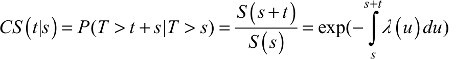
The survival probability P(T>t) quantifies the probability to be alive after a certain time point t, and it can be written in terms of the mortality hazard λ(t) through the relationship 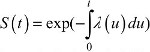. It follows that 1-S(t) quantifies the (cumulative) probability of death before time t, P(T ≤ t). An additional quantity that can be easily derived is the CS,^6–10 CS(t|s), defined as the probability of surviving further “t” years given that a patient has already survived “s” years after the diagnosis:⁷

(1)

It gives an updated survival probability for patients who survived up to time “s” and reflects the impact of late effects, complications or occurrence of late events (eg, recurrences) as their mortality hazard varies over time. This measure can be used as a function of the time point s, at which the prediction is made in order to obtain the probability that a patient survives at least “t” more years⁷ after surviving the first “s” years from diagnosis. It could be useful to compare patient’s prognosis after say 1 year of follow-up, as the mortality hazard is often high during the first year after diagnosis, hence the cohort of patients surviving the first year may have different characteristics compared to the original cohort of patients. This measure is also related to the probability of the remaining life (also known as probability of the residual life), which is defined as 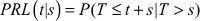. The probability of the remaining life (PRL) is the probability that patients die within “t” years after having already survived “s” years from diagnosis.¹¹

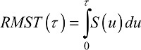
Restricted mean survival time

The mean survival time (MST) is the expected period of time that patients will survive after their cancer diagnosis. The calculation of the MST requires the estimation of the entire survival function (that is, until to the point when the survival probability reaches 0, in other words the follow-up is long enough for all events to be observed). This is an important limitation in practice given that survival data are typically right-censored due to random dropout or limited follow-up. This implies that the right-hand tail of the survival function is usually unobserved (ie, we do not observe the deaths for the whole cohort). The RMST represents an alternative measure that overcomes this limitation^12–17 and is defined as the mean survival time over a prespecified time window [0-τ]. The RMST is interpreted as the τ-year life expectancy. In mathematical terms, the RMST(τ) is defined as

(2)

It can be seen from the previous equation that the RMST is simply the area under the survival curve between time 0 and τ (Figure 1). This measure is defined on the timescale (instead of the probability scale) and is therefore quite attractive due to its simplicity for both interpretation and communication in clinical setting.^14,16,18 Moreover, the RMST is an appealing outcome measure as it produces a single summary value even in cases when the hazard ratio varies with time since diagnosis (ie, nonproportional hazards).^14,19 Therefore, quantifying a difference between treatments using the RMST provides a clinically meaningful measure, compared to an estimated hazard ratio, only relevant in the limited number of scenarios where the proportional hazards assumption is reasonable.

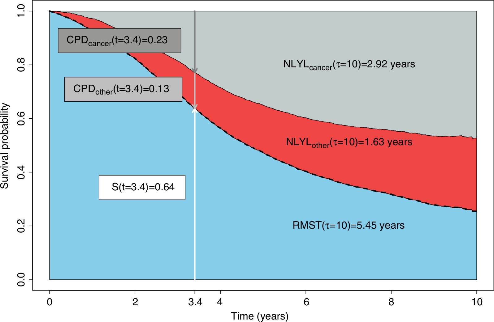Figure 1 Graphical representation of the different measures using simulated data: the overall survival probability (dashed black curve), the 10-year RMST (lower shaded area), the NLYL at 10 years according to each cause (NLYLcancer – upper shaded area and NLYLother – middle shaded area, which sum up to give the RMTL), and the curves of the CPD due to cancer (CPDcancer) and due to other causes (CPDother), using a (reverse) stacked display format. Note: Simulated data were used for this graphical representation; therefore, the values do not match the estimated values from the manuscript (which were based on real data). Abbreviations: CPD, crude probability of death; NLYL, number of life years lost; RMST, restricted mean survival time; RMTL, restricted mean time lost.

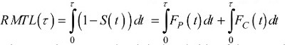
Notice the reversed perspective with the restricted mean time lost (RMTL),¹⁶ , which is interpreted as the expected number of years lost before time τ (compared to an “immortal” cohort). Geometrically, this quantity is the area above the survival curve (Figure 1).

Accounting for competing risks in the relative survival data setting

Net survival

Cancer patients may die from causes other than the cancer under study. However, in the relative survival setting, the cause of death is not available (or unreliable) and the mortality hazards from other causes are provided by the background mortality from the general population to deduce the excess mortality hazard that can be attributed, directly or indirectly, to the cancer under study. In mathematical terms, this means that the overall mortality hazard λ_Oi, for patient i, is the sum of two hazards, the excess hazard λ_Ei (associated to the cancer under study) and the expected hazard λ_Pi(coming from the general population):^20–25

(3)

The expected mortality hazard λ_Pi is assumed to be known. In practice, λ_Pi is usually obtained from life tables built by national statistics institutes and stratified on some sociodemographic variables (such as age, sex, calendar year, deprivation and region).

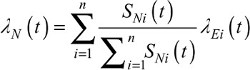
The hazard functions in equation (3) are defined at “individual level”. From this hazard structure in equation (3), we can derive marginal hazard and marginal survival functions (ie, defined at the “population level”). The NS function of a patient i is the survival derived from the excess mortality hazard , while the NS of the whole cohort (ie, marginal) is the average of individual NS functions: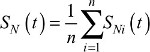. NS does not depend on mortality from other causes,^22,23,26 so it is most useful for comparing different populations after age standardization to account for the difference in the structure of age between populations.^27,28 It estimates the survival that cancer patients would experience if they could only die from the cancer under study. A nonparametric estimator of NS, relying on counting process theory, was proposed by Perme et al.²³ This estimator is based on estimating the cumulative excess hazard in order to deduce the NS of the whole cohort SN(t). The marginal net hazard (ie, defined for the whole cohort) is derived from the marginal NS as a weighted sum of the individuals’ excess hazards (Supplementary materials for more explanations on the formulas):

(4)

It is worth noting that the link between individual and marginal hazards to account for individuals’ heterogeneity also exists in the overall survival setting (Supplementary materials), but is less important to be presented compared to the relative survival setting, as explained later in the manuscript (explained in the “Crude probability of death (CPD)” section).

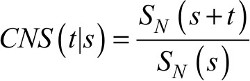
Conditional net survival probability

Analogous to the overall survival setting, the CNS, CNS (t|s) is the probability patients survive further “t” years given that they have already survived “s” years after the diagnosis, but in the hypothetical situation where they could only die from the cancer under study:^29–32

(5)

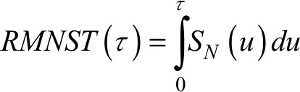
Restricted mean net survival time (RMNST)

Analogous to the derivation of the RMST in the overall survival setting (equation 2), the RMNST is defined in the relative survival setting as

(6)

with the NS function replacing the overall survival from equation (2).

The RMNST represents the mean NS over a prespecified time window [0,τ] and quantifies the mean time patients would survive if they were only exposed to the mortality hazard due to cancer between 0 and τ years from the diagnosis. Given that this measure is not affected by other causes of death, it represents a useful tool for comparing different populations. In addition, this measure can be derived with any NS model, including nonproportional excess hazard models, in contrast to other comparison tools such as log-rank-based test for comparing NS curves which loses power in case of nonproportional hazards.^33,34

Crude probability of death (CPD)

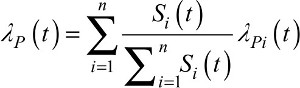
For this measure, we first need to define the marginal cause-specific hazard λ_C(t) and the marginal expected mortality hazard λ_P(t) (ie, defined on the whole population, Supplementary materials). They are also derived from Equation 3:

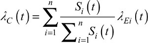(7)

(8)

At this point, it is crucial to highlight the difference between the marginal net hazard λ_N(t) and the marginal cause-specific hazard λ_C(t). Both are based on a weighted average of individuals’ excess hazards,²³ and the difference lies in the weights that multiply the individual excess hazards, which are either based on the individual’s NS, 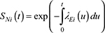or on the individual’s overall survival 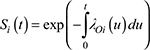(Supplementary materials). In other words, λ_N(t) does not depend on the individuals’ expected mortality hazards, while λ_C(t) does. Notice that if the individual excess hazards are identical for all patients (ie, no heterogeneity observed between patients), then the two population hazards λ_N(t) and λ_C(t) are equal.²³

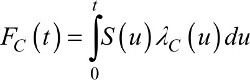
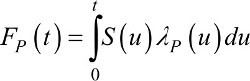
The CPD due to cancer F_C(t) and the CPD due to other causes F_P(t) are defined as

(9)

(10)

The function F_C(t) represents the probability of dying from cancer under study before time t, in the presence of other causes of death. F_P(t) represents the probability of dying from other causes before time t, in the presence of cancer as a cause of death.^35,36 More specifically, by splitting the overall mortality hazard of a group of individuals as the sum of the cause-specific mortality hazard and the other-cause mortality hazard, the probability of death can be written as the sum of the probability of death due to cancer and that due to other causes (Figure 1; Supplementary materials). The crude probability F_C(t) is an indicator relevant to cancer patients interested in their prognosis as well as for health care planning.^{24,35,37–39} In the classical competing risks framework (ie, with known and reliable information on cause of death), this measure is also known as the cause-specific cumulative incidence function^40,41 or the absolute cause-specific risk of death.⁴²

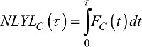
Number of life years lost (NLYL)

The restricted mean of time lost can be decomposed according to the cause of death.⁴³ This decomposition can be extended to the relative survival setting. Since the overall probability of death is equal to the sum of the probability of death from cancer and the probability of death from other causes, 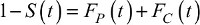, we integrate this function between 0 and τ and decompose the RMTL(τ) (Figure 1) as

(11)

where each term on the right-hand side of the equation corresponds to the mean NLYL due to population mortality and cancer-specific mortality over a t-year time window, respectively.³⁵

(12)

(13)

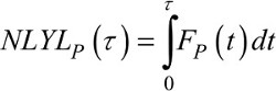
We can also use this decomposition to compare the cancer patients to the general population, in order to quantify how many years of life expectancy patients lose because of the cancer.^43–45 Rearranging Equation 11, the NLYL due to the cancer before time τ, NLYL_C(τ), is defined as

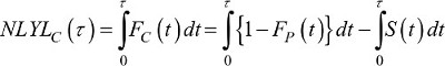(14)

where the quantity 1-F_P(t) can be replaced by SP(t), ie, the classical survival function using the population mortality rates λ_P. Equation 14 shows that the NLYL due to the cancer before time τ is simply the difference between the area under the curve of the population survival minus the area under the curve of the overall survival (ie, the area between the two curves).^46,47

Estimation

In both settings (overall and relative survival) and for each measure summarized in Table 1, we followed the same principle of estimation; we used nonparametric estimators and plugged them in the corresponding formulas. In the overall survival setting, we used the nonparametric Kaplan–Meier estimator^40,48 for overall survival and CS probabilities and for RMST(τ). In the relative survival setting, we used the nonparametric Pohar-Perme estimator²³ of NS, CNS and RMNST(τ). For the CPD and the NLYL, we used an Aalen–Johansen type estimator defined in the relative survival setting. All analyses were done with the R software (R Foundation for Statistical Computing, Vienna, Austria), version 3.2.4 and the packages survival and relsurv. For the standard errors of the estimates, we used analytical formulas when available, or we used nonparametric boostrap⁴⁹ using the R-package boot (for the CNS and the RMNST). Supplementary materials detail the R code to perform the estimations.

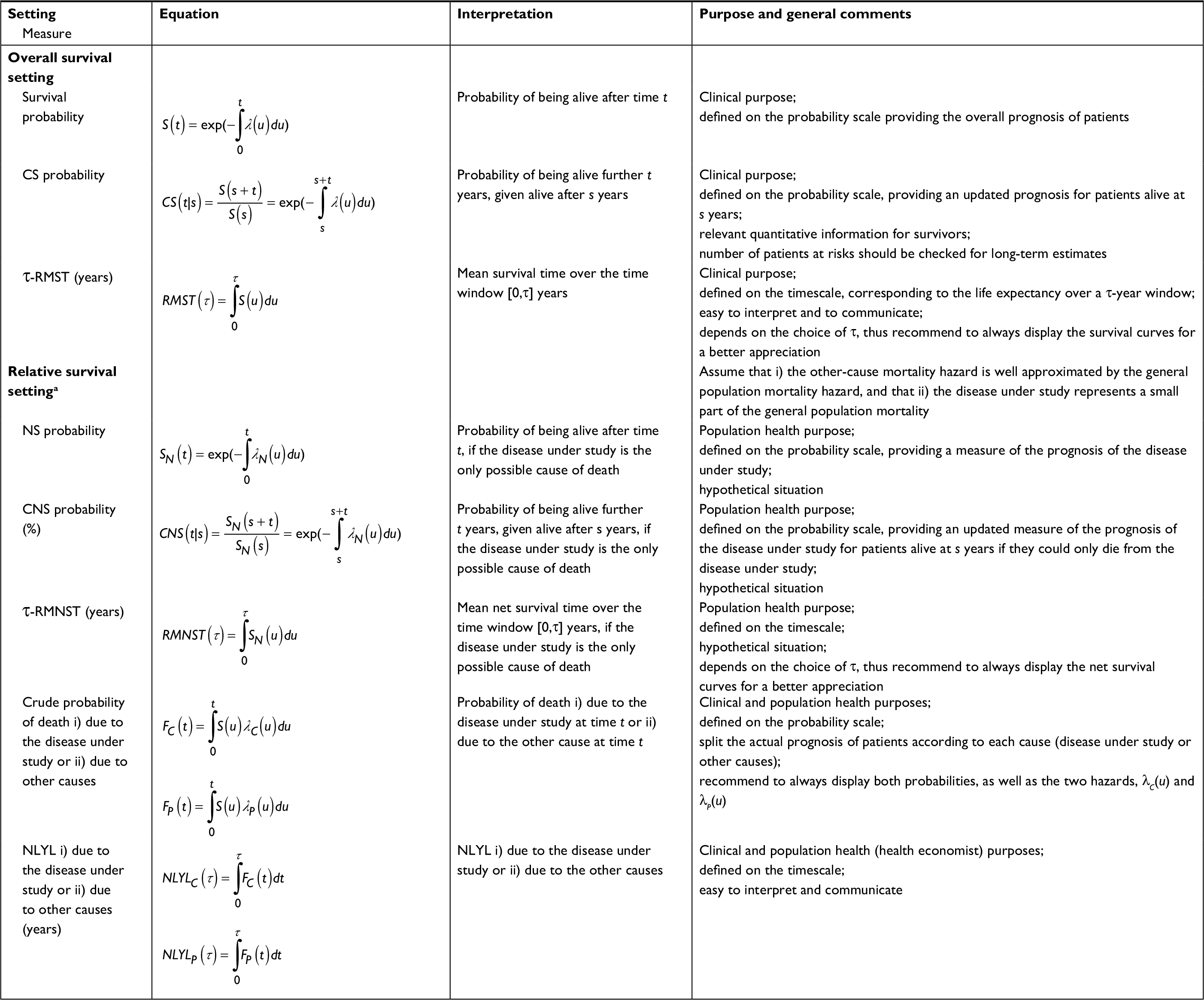Table 1 Equation, interpretation and general comments of the statistical measures detailed in this work for summarizing survival data, where l defines the overall mortality hazard, and λN(u) the net mortality hazard due to the disease under study. The cumulative net hazard is estimated using the Pohar-Perme estimator.23 Refer the “Theoretical framework” section for the definition of λN(u), λC(u) and λP(u). Notes: aRelative survival setting corresponds to the particular competing risk setting in which information of the cause of death is not reliably known. This situation is common, for example, when analyzing population-based cancer registry data. Abbreviations: CS, conditional survival; CNS, conditional net survival; NLYL, number of life years lost; NS, net survival; RMST, restricted mean survival time; RMNST, restricted mean net survival time.

Material for the illustration

To illustrate the usefulness and the interpretations of the different measures, we analyzed records of males diagnosed with colon cancer, obtained from the England population-based cancer registry. We aimed to describe socioeconomic disparities in (cancer) survival. We limited the analysis to the patients diagnosed between 2001 and 2003 and aged between 15 and 80 years old at diagnosis and followed up up to December 31, 2014. Thus, all patients had a minimum potential follow-up of 10 years. Estimation in the relative survival setting used life tables stratified by age, sex, calendar year, Government office region and deprivation.

Patients were categorized in five socioeconomic status groups (from the least deprived group, level 1, to the most deprived group, level 5) using national quintiles of the income domain score of the Index of Multiple Deprivation (IMD 2004),⁵⁰ which is a score defined at the lower super output area level in England (geographical area of approximately 1,500 inhabitants). The income domain score combines five indicators, and it measures the proportion of the population in an area experiencing deprivation related to low income. When measured at a relatively small geographical level, this ecological deprivation score is considered as a good proxy of individual deprivation, while additionally measuring the patients’ social and economic environment.^51,52 Methodological guidelines describe the use of such ecological deprivation scores in the context of cancer survival and discuss their limits.⁵³

Ethics approval

We obtained the ethical and statutory approvals required for this research (PIAG 1-05(c)/2007; ECC 1-05(a)/2010; ethical approval updated April 6, 2017 (REC 13/LO/0610)), from the Confidentiality Advisory Group (CAG) part of the Health Research Authority (HRA).

Results

A total of 14,316 deaths out of 19,853 patients occurred over the study period. The group aged between 65 and 74 years constituted over 40% of the patients under study (Table 2).

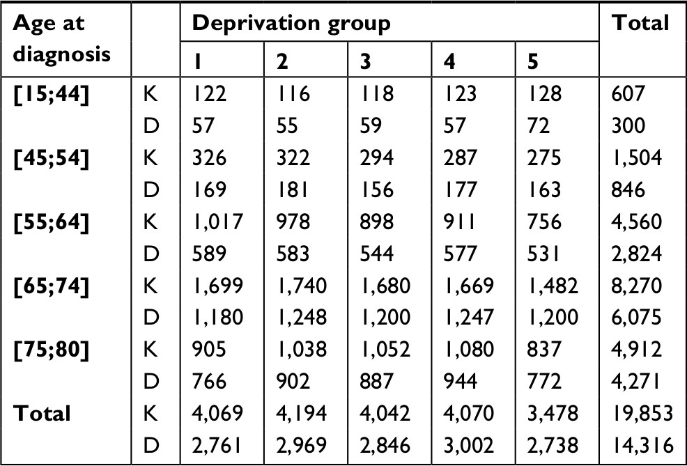Table 2 Number of cases (K) and deaths (D) observed before December 31, 2014, in men aged between 15 and 80 years old at diagnosis and diagnosed between 2001 and 2003 in England, by deprivation and age at diagnosis groups (Deprivation 1 corresponding to the less deprived and 5 to the most deprived)

Overall survival setting

Survival and CS probabilities

The 10-year overall survival probability for all ages combined was 0.36 (95% confidence interval [CI]: 0.34, 0.37) for deprivation group 1, and 0.25 (95% CI: 0.24, 0.27) for deprivation group 5 (Table 3), and the 10-year overall survival probabilities by deprivation and age group are detailed in Table S1 and Figure S1.

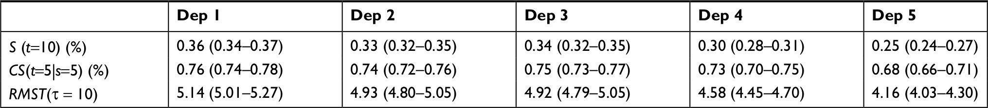Table 3 Measures estimated in the classical survival setting, in men aged between 15 and 80 years old at diagnosis by deprivation group (Dep), with their 95% CIs: the survival probability at 10 years after diagnosis S(t=10), the conditional probability of surviving further t=5 years given that a patient already survived s = 5 years CS(t=5|s=5), and the restricted mean survival time at 10 years RMST(τ = 10) Abbreviations: CS, conditional survival; RMST, restricted mean survival time.

The CS gives a more optimistic picture of the prognosis, even though the deprivation disparities remain substantial: once patients survived the first 5 years, the probability to survive 5 more years CS(5|5) was 0.76 (95% CI: 0.74, 0.78) for the least deprived and 0.68 (95% CI: 0.66, 0.71) for the most deprived (Table 3). The deprivation disparity was observed in all age groups (Table S2; Figure S2).

RMST

We estimated the 10-year RMST by deprivation group, for all ages combined (Table 3) and by age group (Table S3; Figure S3). The RMST at 10 years was estimated as 5.14 years, (95% CI: 5.01, 5.27) for the least deprived group compared to 4.16 years (95% CI: 4.03, 4.30) for the most deprived group of patients (Table 3).

While the 10-year RMSTs were almost similar across deprivation categories in the group aged 15–44 years, they differ by more than 1 year in the age groups 55–64 and 65–74 years. Patients aged 55–64 years survived on average 5.76 years (95% CI: 5.5, 6.02) in the least deprived group vs 4.73 years (95% CI: 4.43, 5.03) in the most deprived group of patients (Table S3). Patients aged 65–74 years survived on average 5.15 years (95% CI: 4.95, 5.34) in the least deprived group vs 4.04 years (95% CI: 3.83, 4.24) in the most deprived group.

Relative survival setting

NS and CNS probabilities

The 10-year NS still displays a clear disparity by deprivation group even though slightly reduced compared to the overall survival (Table 4). These disparities of NS between deprivation groups remained by age group (Table S4; Figure S4). However, the deprivation disparity almost disappear on the CNS(5|5) for all ages combined (Table 4), and also by age group for patients younger than 74 years (Table S5; Figure S5). A nice illustration is given by cancer patients aged 55–64 years: the CNS(5|1) is quite different between the most deprived group and the other groups. But as the time we are conditioning on passes, the difference narrows (Table S5; Figure S5). It shows that most of the difference between deprivation groups happened during the beginning of the follow-up, while after 5 years, the excess mortality hazard was almost the same in the different deprivation groups, except for the group of age 75–80 years.

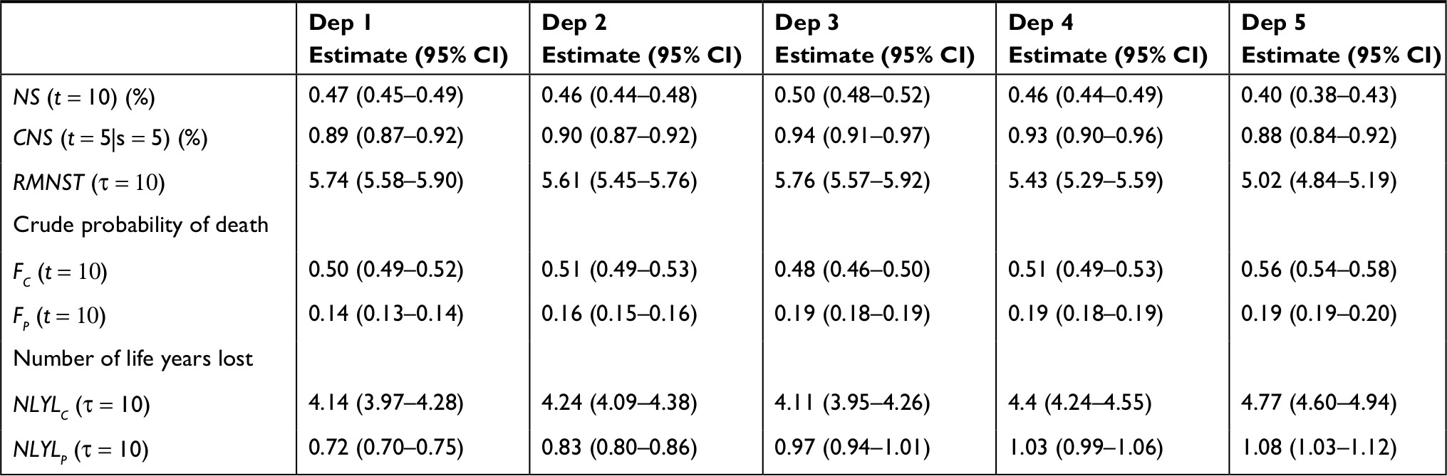Table 4 Measures estimated in the relative survival setting, in men aged between 15 and 80 years old at diagnosis by deprivation group (Dep), with their 95% CIs: the NS probability at 10 years after diagnosis NS(t = 10), the CNS, CNS(t = 5|s = 5), the RMNST at 10 years RMNST (τ = 10), the crude probability of death at 10 years for cancer FC(t = 10) and other causes FP(t = 10) , and the number of life years lost due to cancer NLYLC(τ = 10) and due to other causes NLYLP(τ = 10) over a 10-year time window Abbreviations: CNS, conditional net survival; NLYL, number of life years lost; NS, net survival; RMNST, restricted mean net survival time.

RMNST

The RMNST at 10 years quantifies the average time patients would survive if they were only exposed to cancer-specific mortality during the next 10 years. Between the least and most deprived groups, a difference of 0.7 years was estimated: 5.74 years (95% CI: 5.58, 5.90) vs 5.02 years (95% CI: 4.84, 5.19) (Table 4). Differences in RMNST at 10 years were observed across all age groups; RMNST decreases while deprivation increases, with a steeper decrease for the most deprived group (Table S6; Figure S6).

CPD

The CPD gives an overall picture of the patients’ prognosis. All ages combined, the CPD from cancer 10 years after diagnosis was estimated as 0.50 (95% CI: 0.49, 0.52) for the least deprived and 0.56 (95% CI: 0.54, 0.58) for the most deprived (Table 4), while the CPD from other causes at 10 years was 0.14 (95% CI: 0.13, 0.14) for deprivation group 1 and 0.19 (95% CI: 0.19, 0.20) for deprivation group 5. We contrasted graphically the prognosis of death from cancer and from other causes, between the least deprived group and the most deprived group (Figure S7). By age group, the differences between the least and the most deprived groups were more pronounced for patients aged 55–64 and 65–74 years, with substantial differences in both CPD from cancer and from other causes (Table S7).

NLYL

Disparities of survival between deprivation groups could also be quantified using the NLYL due to cancer and other causes. For the most deprived, the NLYL at 10 years due to cancer was 4.14 years (95% CI: 3.97, 4.28) and was 0.72 years (95% CI: 0.70, 0.75) due to other causes, compared to 4.77 (95% CI: 4.60, 4.94) and 1.08 (95% CI: 1.03; 1.12) in the least deprived group, respectively (Table 3). Those disparities varied by age group. In the 55–64 years age group, the NLYL due to cancer was around 4 years for deprivation groups 1–4, and it was more than 4.5 years for the most deprived. The disparities in NLYL due to other causes were also substantial in age groups 55–64 and 65–74 years (Table S8; Figure S8).

Discussion

Survival data are typically summarized through the probability of being alive after a certain amount of time. Even though this probability is a measure which cannot be directly assigned to individual patients (because of many unknown prognostic factors), it represents the main indicator patients (and their clinicians) are interested in. Nevertheless, alternative measures can be useful as they provide additional insights into the data as well as alternative ways of communicating cancer prognostic information to different target audiences. This need for presenting cancer survival statistics in different and complementary ways to patients, clinicians and policy makers becomes even more relevant as the burden of cancer rises worldwide.³⁹ Using colon cancer data of men diagnosed in England between 2001 and 2003 and followed up for 10 years, we illustrated the use of these alternative measures (Table 1). Overall survival shows clear deprivation-related pattern, and even after conditioning on being alive at 5 years after diagnosis, the probability to be alive after 5 more years still displays deprivation disparities (CS). The same is observed with the RMST, while quantified on a timescale. However, those measures are not able to separate the deprivation disparities associated to cancer-specific mortality from that due to other causes. Accounting for the differences in expected mortality between deprivation groups is feasible using the relative survival setting (and its associated methodology); the obtained results in our example, however, do not explain much of these disparities. This methodology also allows to provide absolute risk of death for patients according to the cause of death, namely, cancer and other causes. Those absolute risks can be translated on the timescale using the NLYLs. It is however important to bear in mind that, when interest lies in comparing two populations, the use of NS methods (and other related measures such as CNS or RMNST) does not prevent to use conventional age standardization to account for differences in the age structure of the population.

We propose to (broadly) classify these alternative measures into two groups: those with a clinical perspective (for patients and clinicians) and those with a population health perspective (for health policy makers and economic evaluations).

From a clinical perspective, the CS is a measure providing an updated picture of the prognosis and thus a more hopeful value to communicate to patients, along their cancer pathway.⁷ Moreover, the CS could easily be extended to different scenarios, such as the recurrence-free survival.⁵⁴ When interest lies in detailing the prognosis according to the cause of death, the crude probabilities of death complement the overall survival, as it distinguishes death from cancer to death from other causes. The CPD is a useful measure of the absolute risk of death for cancer patients and has been shown to improve patient’s understanding of survival statistics.⁵⁵ Still within a clinical perspective, intuitive and “easy to communicate” measures are those based on a metric of time (instead of probability), such as the RMST over a τ-year period of time and the NLYL due to each cause. Those metrics heλ_P to quantify the loss in life expectancy (within a predefined time frame) between different groups.

From a population health perspective, the measures based on the net survival (NS, CNS and RMNST) are useful for comparison purposes. They allow comparisons of different populations, within a country (different periods or subpopulations) or between countries (for example, to compare the performance of their health care system in managing cancer patients). Those comparisons are not affected by the differences in background mortality between populations. The NS quantifies the differences on a probability scale, the RMNST on a timescale, while the CNS gives an updated picture of the NS over time since diagnosis. A way of deriving a CI for the difference between (say) the NS in deprivation group 1 and the NS in deprivation group 5 could be the use of resampling methods, such as nonparametric bootstrap. One should, however, notice that this corresponds to a single time point difference, while testing difference between deprivation groups of the NS curves would be more of interest.^33,34 Comparing RMNST curves would be an interesting extension of a work already done for the RMST,¹⁷ where the authors proposed a more sophisticated method for deriving simultaneous CIs. Other authors derived statistical tests and procedures when comparing the RMST in the context of clinical trials.^56,57 Measures based on NS are defined in a hypothetical world where patients could only die from their disease. Thus, their usefulness is mostly for comparisons in population health perspectives, but not for patient’s actual prognosis. If one is interested in quantifying how a given variable affects the cancer-specific mortality hazard (etiological assessment), the excess mortality hazard is the quantity to use,^25,58–60 which is in line with the recommendation usually made in the classical competing risks setting when comparing cause-specific hazards instead of cumulative incidence functions.^41,61 The excess mortality hazard heλ_Ps to assess the cancer prognosis for patients, ie, the lethality of the cancer.

The perspective of the health economist is more, for example, in quantifying the burden of a given disease on the society and how that disease affects the population, possibly during their working life. In that sense, the NLYL might be of interest to quantify the economic cost of patients’ years of life lost at working age because of the disease. Health policy makers may use NLYL to quantify, for instance, the number of life years that could be saved by allocating more resources or reforming/changing the health care system.

We illustrated the use of these measures in cancer epidemiology, but they could also be used in other clinical areas, where the assumption that patients can only die from the disease under study is still reasonable, such as survival after a HIV infection or following a stroke or a kidney disease diagnosis. Applying the CS and the RMST in those clinical areas can be done as detailed in the previous sections. For the relative survival setting, some research has already been done to estimate the excess mortality hazard in HIV-infected patients,^62,63 in patients diagnosed with a kidney disease,^64–67 and for patients following myocardial infarction,^68,69 or a stroke.⁷⁰ The other measures available in the relative survival setting (CNS, RMNST, CPD and NLYL) have received much less attention. However, one should be careful when using the excess mortality hazard method in a given clinical area, as one key assumption is the availability of a good approximation (with life tables) of the mortality hazard due to other causes. Depending on the context/geographical area, the life table may not provide a reasonable approximation of the mortality from other causes; for example, the life table in some sub-Saharan countries is hugely impacted by HIV mortality. Thus, the excess mortality hazard approach would need to account for this, if one is interested in estimating the excess mortality due to HIV infection.⁷¹

We used observational data to illustrate the deprivation disparities in survival using different measures, and these measures were used as exploratory/descriptive tools rather than explanatory tools. Indeed, evaluating the effect of deprivation on these colon cancer disparities would call for methods besides standardization via life table data to account for confounding. Recent literature employs some of these alternative measures coupled with causal inference techniques. For instance, causal inference methods using the RMST in the overall survival setting have been developed recently.^72,73 There are also causal inference studies in the context of the competing risks setting with known cause of death.⁷⁴ The restricted mean residual lifetime has also been combined with g-computation to estimate an average causal effect.⁷⁵

We presented and described the use of different ways for summarizing cancer survival data, each of them contributing differently to provide information to patients, clinicians, health policy makers and health economists on the disease disparities in deprivation groups. Even though we illustrated the use of these measures using nonparametric estimators, parametric and semiparametric hazard-based regression models could be also used. We provided the R code for implementing all these measures with the hope that the reader will start applying and comparing different and complementary measures in the presentation of survival data.

Abbreviations

CS, conditional survival; CNS, conditional net survival; CPD, crude probability of death; NLYL, number of life years lost; NS, net survival; MST, mean survival time; PRL, probability of the remaining life; RMST, restricted mean survival time; RMNST, restricted mean net survival time; RMTL, restricted mean time lost.

Acknowledgments

The authors thank Jacques Estève for useful advice on the first draft of the manuscript, and the members of the Cancer Survival Group of the London School of Hygiene & Tropical Medicine for interesting discussion on the topic. This research was supported by Cancer Research UK grant number C7923/A18525. The findings and conclusions in this report are those of the authors and do not necessarily represent the views of Cancer Research UK. Miguel-Angel Luque-Fernandez is supported by the Spanish National Institute of Health Carlos III Miguel Servet I Investigator Award (CP17/00206). This research has been finalized while Aurélien Belot was fellow at the Collegium - Lyon Institute for Advanced Study 2018-2019.

Author contributions

AB, MALF and BR developed the concept and design of the study. AB and AN were involved in the data preparation, carried out the data analysis and wrote the manuscript. All authors contributed to data analysis, drafting and revising the article, gave final approval of the version to be published, and agree to be accountable for all aspects of the work.

Disclosure

The authors report no conflicts of interest in this work.

References

1.		Brewster DH, Coebergh JW, Storm HH. Population-based cancer registries: the invisible key to cancer control. Lancet Oncol. 2005;6(4):193–195.
2.		Percy C, Stanek E, Gloeckler L. Accuracy of cancer death certificates and its effect on cancer mortality statistics. Am J Public Health. 1981;71(3):242–250.
3.		Mant J, Wilson S, Parry J, et al. Clinicians didn’t reliably distinguish between different causes of cardiac death using case histories. J Clin Epidemiol. 2006;59(8):862–867.
4.		Johnson CJ, Hahn CG, Fink AK, German RR. Variability in cancer death certificate accuracy by characteristics of death certifiers. Am J Forensic Med Pathol. 2012;33(2):137–142.
5.		Schaffar R, Rapiti E, Rachet B, Woods L. Accuracy of cause of death data routinely recorded in a population-based cancer registry: impact on cause-specific survival and validation using the Geneva Cancer Registry. BMC Cancer. 2013;13:609.
6.		Skuladottir H, Olsen JH. Conditional survival of patients with the four major histologic subgroups of lung cancer in Denmark. J Clin Oncol. 2003;21(16):3035–3040.
7.		Hieke S, Kleber M, König C, Engelhardt M, Schumacher M. Conditional Survival: A Useful Concept to Provide Information on How Prognosis Evolves over Time. Clin Cancer Res. 2015;21(7):1530–1536.
8.		Zabor EC, Gonen M, Chapman PB, Panageas KS. Dynamic prognostication using conditional survival estimates. Cancer. 2013;119(20):3589–3592.
9.		Xing Y, Chang GJ, Hu CY, et al. Conditional survival estimates improve over time for patients with advanced melanoma: results from a population-based analysis. Cancer. 2010;116(9):2234–2241.
10.		Haydu LE, Scolyer RA, Lo S, et al. Conditional Survival: An Assessment of the Prognosis of Patients at Time Points After Initial Diagnosis and Treatment of Locoregional Melanoma Metastasis. J Clin Oncol. 2017;35(15):1721–1729.
11.		Rubio FJ, Hong Y. Survival and lifetime data analysis with a flexible class of distributions. J Appl Stat. 2016;43(10):1794–1813.
12.		Karrison TG. Use of Irwin’s restricted mean as an index for comparing survival in different treatment groups--interpretation and power considerations. Control Clin Trials. 1997;18(2):151–167.
13.		Irwin JO. The standard error of an estimate of expectation of life, with special reference to expectation of tumourless life in experiments with mice. J Hyg. 1949;47(2):188–189.
14.		Royston P, Parmar MK. The use of restricted mean survival time to estimate the treatment effect in randomized clinical trials when the proportional hazards assumption is in doubt. Stat Med. 2011;30(19):2409–2421.
15.		Andersen PK, Hansen MG, Klein JP. Regression analysis of restricted mean survival time based on pseudo-observations. Lifetime Data Anal. 2004;10(4):335–350.
16.		Uno H, Claggett B, Tian L, et al. Moving beyond the hazard ratio in quantifying the between-group difference in survival analysis. J Clin Oncol. 2014;32(22):2380–2385.
17.		Zhao L, Claggett B, Tian L, et al. On the restricted mean survival time curve in survival analysis. Biometrics. 2016;72(1):215–221.
18.		Eng KH, Seagle BL. Covariate-Adjusted Restricted Mean Survival Times and Curves. J Clin Oncol. 2017;35(4):465–466.
19.		Royston P, Parmar MK. Restricted mean survival time: an alternative to the hazard ratio for the design and analysis of randomized trials with a time-to-event outcome. BMC Med Res Methodol. 2013;13:152.
20.		Berkson J, Gage RP. Calculation of survival rates for cancer. Proc Staff Meet Mayo Clin. 1950;25(11):270–286.
21.		Ederer F, Axtell LM, Cutler SJ. The relative survival rate: a statistical methodology. Natl Cancer Inst Monogr. 1961;6:101–121.
22.		Pohar Perme M, Estève J, Rachet B. Analysing population-based cancer survival – settling the controversies. BMC Cancer. 2016;16(1):933.
23.		Perme MP, Stare J, Estève J. On estimation in relative survival. Biometrics. 2012;68(1):113–120.
24.		Mariotto AB, Noone AM, Howlader N, et al. Cancer survival: an overview of measures, uses, and interpretation. J Natl Cancer Inst Monogr. 2014;2014(49):145–186.
25.		Estève J, Benhamou E, Croasdale M, Raymond L. Relative survival and the estimation of net survival: elements for further discussion. Stat Med. 1990;9(5):529–538.
26.		Danieli C, Remontet L, Bossard N, Roche L, Belot A. Estimating net survival: the importance of allowing for informative censoring. Stat Med. 2012;31(8):775–786.
27.		de Angelis R, Sant M, Coleman MP, et al. Cancer survival in Europe 1999-2007 by country and age: results of EUROCARE-5 – a population-based study. Lancet Oncol. 2014;15(1):23–34.
28.		Allemani C, Weir HK, Carreira H, et al. Global surveillance of cancer survival 1995–2009: analysis of individual data for 25, 676, 887 patients from 279 population-based registries in 67 countries (CONCORD-2). Lancet. 2015;385(9972):977–1010.
29.		Bouvier AM, Remontet L, Hedelin G, et al. Conditional relative survival of cancer patients and conditional probability of death: a French National Database analysis. Cancer. 2009;115(19):4616–4624.
30.		Shack L, Bryant H, Lockwood G, Ellison LF. Conditional relative survival: a different perspective to measuring cancer outcomes. Cancer Epidemiol. 2013;37(4):446–448.
31.		Janssen-Heijnen ML, Gondos A, Bray F, et al. Clinical relevance of conditional survival of cancer patients in europe: age-specific analyses of 13 cancers. J Clin Oncol. 2010;28(15):2520–2528.
32.		Yu XQ, Baade PD, O’Connell DL. Conditional survival of cancer patients: an Australian perspective. BMC Cancer. 2012;12(1):460.
33.		Grafféo N, Castell F, Belot A, Giorgi R. A log-rank-type test to compare net survival distributions. Biometrics. 2016;72(3):760–769.
34.		Pavlicˇ K, Perme MP. On comparison of net survival curves. BMC Med Res Methodol. 2017;17(1):79.
35.		Cronin KA, Feuer EJ. Cumulative cause-specific mortality for cancer patients in the presence of other causes: a crude analogue of relative survival. Stat Med. 2000;19(13):1729–1740.
36.		Lambert PC, Dickman PW, Nelson CP, Royston P. Estimating the crude probability of death due to cancer and other causes using relative survival models. Stat Med. 2010;29(7–8):885–895.
37.		Lee M, Cronin KA, Gail MH, Feuer EJ. Predicting the absolute risk of dying from colorectal cancer and from other causes using population-based cancer registry data. Stat Med. 2012;31(5):489–500.
38.		Charvat H, Bossard N, Daubisse L, Binder F, Belot A, Remontet L. Probabilities of dying from cancer and other causes in French cancer patients based on an unbiased estimator of net survival: a study of five common cancers. Cancer Epidemiol. 2013;37(6):857–863.
39.		Eloranta S, Adolfsson J, Lambert PC, et al. How can we make cancer survival statistics more useful for patients and clinicians: an illustration using localized prostate cancer in Sweden. Cancer Causes Control. 2013;24(3):505–515.
40.		Geskus RB. Data Analysis with Competing Risks and Intermediate States. Boca Raton: Taylor & Francis; 2016:247.
41.		Andersen PK, Geskus RB, de Witte T, Putter H. Competing risks in epidemiology: possibilities and pitfalls. Int J Epidemiol. 2012;41(3):861–870.
42.		Benichou J, Gail MH. Estimates of absolute cause-specific risk in cohort studies. Biometrics. 1990;46(3):813–826.
43.		Andersen PK. Decomposition of number of life years lost according to causes of death. Stat Med. 2013;32(30):5278–5285.
44.		Hakama M, Hakulinen T. Estimating the expectation of life in cancer survival studies with incomplete follow-up information. J Chronic Dis. 1977;30(9):585–597.
45.		Chu PC, Wang JD, Hwang JS, Chang YY. Estimation of life expectancy and the expected years of life lost in patients with major cancers: extrapolation of survival curves under high-censored rates. Value Health. 2008;11(7):1102–1109.
46.		Baade PD, Youlden DR, Andersson TM, et al. Estimating the change in life expectancy after a diagnosis of cancer among the Australian population. BMJ Open. 2015;5(4):e006740.
47.		Dehbi HM, Royston P, Hackshaw A. Life expectancy difference and life expectancy ratio: two measures of treatment effects in randomised trials with non-proportional hazards. BMJ. 2017;357:j2250.
48.		Kalbfleisch JD, Prentice RL. The Statistical Analysis of Failure Time Data. 2nd ed. Hoboken, NJ: John Wiley; 2002.
49.		Diciccio TJ, Efron B. Bootstrap confidence intervals. Statist Sci. 1996;11(3):189–228.
50.		Neighbourhood Renewal Unit. The English Indices of Deprivation 2004 (revised). London: Office for the Deputy Prime Minister; 2004.
51.		Woods LM, Rachet B, Coleman MP. Choice of geographic unit influences socioeconomic inequalities in breast cancer survival. Br J Cancer. 2005;92(7):1279–1282.
52.		Diez Roux AV. Investigating neighborhood and area effects on health. Am J Public Health. 2001;91(11):1783–1789.
53.		Belot A, Remontet L, Rachet B, et al. Describing the association between socioeconomic inequalities and cancer survival: methodological guidelines and illustration with population-based data. Clin Epidemiol. 2018;10:561–573.
54.		Zamboni BA, Yothers G, Choi M, et al. Conditional survival and the choice of conditioning set for patients with colon cancer: an analysis of NSABP trials C-03 through C-07. J Clin Oncol. 2010;28(15):2544–2548.
55.		Fagerlin A, Zikmund-Fisher BJ, Ubel PA. HeλPing patients decide: ten steps to better risk communication. J Natl Cancer Inst. 2011;103(19):1436–1443.
56.		Horiguchi M, Cronin AM, Takeuchi M, Uno H. A flexible and coherent test/estimation procedure based on restricted mean survival times for censored time-to-event data in randomized clinical trials. Stat Med. 2018;37(15):2307–2320.
57.		Tian L, Fu H, Ruberg SJ, Uno H, Wei LJ. Efficiency of two sample tests via the restricted mean survival time for analyzing event time observations. Biometrics. 2018;74(2):694–702.
58.		Remontet L, Bossard N, Belot A, Estève J; French network of cancer registries FRANCIM. An overall strategy based on regression models to estimate relative survival and model the effects of prognostic factors in cancer survival studies. Stat Med. 2007;26(10):2214–2228.
59.		Charvat H, Remontet L, Bossard N, et al. A multilevel excess hazard model to estimate net survival on hierarchical data allowing for non-linear and non-proportional effects of covariates. Stat Med. 2016;35(18):3066–3084.
60.		Luque-Fernandez MA, Belot A, Quaresma M, Maringe C, Coleman MP, Rachet B. Adjusting for overdispersion in piecewise exponential regression models to estimate excess mortality rate in population-based research. BMC Med Res Methodol. 2016;16(1):129.
61.		Putter H, Fiocco M, Geskus RB. Tutorial in biostatistics: competing risks and multi-state models. Stat Med. 2007;26(11):2389–2430.
62.		Bhaskaran K, Hamouda O, Sannes M, et al. Changes in the risk of death after HIV seroconversion compared with mortality in the general population. JAMA. 2008;300(1):51–59.
63.		Mcdavid Harrison K, Ling Q, Song R, Hall HI. County-level socioeconomic status and survival after HIV diagnosis, United States. Ann Epidemiol. 2008;18(12):919–927.
64.		Elie C, de Rycke Y, Jais J, Landais P. Appraising relative and excess mortality in population-based studies of chronic diseases such as end-stage renal disease. Clin Epidemiol. 2011;3:157–169.
65.		Nordio M, Limido A, Maggiore U, et al. Survival in patients treated by long-term dialysis compared with the general population. Am J Kidney Dis. 2012;59(6):819–828.
66.		Trébern-Launay K, Giral M, Dantal J, Foucher Y. Comparison of the risk factors effects between two populations: two alternative approaches illustrated by the analysis of first and second kidney transplant recipients. BMC Med Res Methodol. 2013;13(1):102.
67.		Gibertoni D, Mandreoli M, Rucci P, et al. Excess mortality attributable to chronic kidney disease. Results from the PIRP project. J Nephrol. 2016;29(5):663–671.
68.		Nelson CP, Lambert PC, Squire IB, Jones DR. Relative survival: what can cardiovascular disease learn from cancer? Eur Heart J. 2008;29(7):941–947.
69.		Alabas OA, Gale CP, Hall M, et al. Sex Differences in Treatments, Relative Survival, and Excess Mortality Following Acute Myocardial Infarction: National Cohort Study Using the SWEDEHEART Registry. J Am Heart Assoc. 2017;6(12):e007123.
70.		Hardie K, Hankey GJ, Jamrozik K, Broadhurst RJ, Anderson C. Ten-year survival after first-ever stroke in the Perth community stroke study. Stroke. 2003;34(8):1842–1846.
71.		Brinkhof MW, Boulle A, Weigel R, et al. Mortality of HIV-infected patients starting antiretroviral therapy in sub-Saharan Africa: comparison with HIV-unrelated mortality. PLoS Med. 2009;6(4):e1000066.
72.		Chen PY, Tsiatis AA. Causal inference on the difference of the restricted mean lifetime between two groups. Biometrics. 2001;57(4):1030–1038.
73.		Zhang M, Schaubel DE. Double-robust semiparametric estimator for differences in restricted mean lifetimes in observational studies. Biometrics. 2012;68(4):999–1009.
74.		Calkins KL, Canan CE, Moore RD, Lesko CR, Lau B. An application of restricted mean survival time in a competing risks setting: comparing time to ART initiation by injection drug use. BMC Med Res Methodol. 2018;18(1):27.
75.		Mansourvar Z, Martinussen T. Estimation of average causal effect using the restricted mean residual lifetime as effect measure. Lifetime Data Anal. 2017;23(3):426–438.