Sample size and power considerations for ordinary least squares interrupted time series analysis: a simulation study

Introduction

Interrupted time series (ITS) analysis is being increasingly used in epidemiology.^1–3 It is an accessible and intuitive method that can be straightforward to implement and has considerable strengths.⁴ A common application is when population-level repeated measures of an outcome and/or exposure are available over time, both before and after some well-defined intervention such as a health policy change^1,2,5 or a naturally occurring event of interest.^6,7

Despite the substantial growth in the use of ITS methods, relatively little practical guidance has been developed in terms of methodological standards within the ITS framework,^1,3 including a scarcity of guidance on required sample size. Sample size planning is often a key component of designing a study and should be conducted prior to analysis,⁸ although this is an aspect very often overlooked in ITS studies, with many being underpowered.⁹

Information on the power associated with various numbers of repeated measures of an outcome (ie, time points) has been previously reported,¹⁰ with rules of thumb concerning the minimum number of pre- and post-intervention time points needed, such as 3,³ 6,¹¹ 8,¹² and ≥10.⁹ However, researchers seeking to aggregate patient-level data into a population-level time series to conduct an ITS are confronted with the practical issue of considering a suitable underlying sample size of subjects/patients per aggregate time point.¹³ Although longer time series have been shown to have more power than shorter time series, it seems reasonable to propose that ITS analyses (even those with many time points) with only a small number of subjects per time point may contain so much noise as to render it improbable of detecting a true impact of an intervention under study. Although the ITS method has many strengths, if a given analysis is not adequately powered it may lead to publication of weak and spurious findings.^14,15

Given this paucity of guidance on sample size calculation, our aim in this study was to use a simulation approach to estimate power in an ITS analysis case study of repeated measures of cumulative incidence generated from routinely collected health care data. We aimed to quantify the power available in relation to the underlying sample size per time point, while varying a number of other key parameters of interest. Furthermore, we set out to make available Stata code to be readily usable by epidemiologists as a tool to generate estimates of required sample size for similar ITS applications.

Methods

Study design

We used Monte Carlo simulations, the strengths of which have been well described previously.^16,17 Briefly, simulation studies involve generating data with known characteristics defined by prespecified input parameter values. Consequently, because the truth regarding these characteristics is known, it is possible to empirically evaluate the performance of a given statistical model when fitted to the simulated data.^18,19

Aims

Our aim was to describe the power associated with the mean sample size per time point to detect a change in 1) level and 2) trend in an outcome (cumulative incidence) following a defined intervention in the ITS framework, using ordinary least squares (OLS) regression. We considered a range of values for various other factors such as total number of time points, effect size, and location of intervention in the time series. We set out to apply the methods within the context of a specific case study using a recent ITS analysis, where we evaluated the impact of a UK National Institute for Health and Care Excellence (NICE) technology appraisal on the cumulative incidence of joint replacement within the Clinical Practice Research Datalink (CPRD).²⁰

ITS scenarios

There are many factors within an OLS ITS framework that could conceivably influence the power to detect the impact of an intervention. Although the following is not an exhaustive list, we here describe the main factors that we investigated:

1. Total number of time points in the time series, N (Figure 1A and B): as described in the “Introduction” section, the ITS approach relies on repeated observations of an outcome event over time, usually at equally spaced intervals such as days, weeks, months, quarters, or years. We investigated nine values for the total number of time points (N), ranging from 6 to 50.
2. Number of subjects per time point, n (Figure 1C and D): the sample size per time point will impact the accuracy of outcome estimates and hence the dispersion of a given time series. It is therefore an important factor influencing the power to detect an “interruption”. We investigated 11 values for n, ranging from approximately 150 to 5,700 patients per time point, which for our specific case study corresponded to a mean number of outcome events per time point that ranged from 5 to 200 (Supplementary materials).
3. Nature of intervention impact (Figure 1A–D): the impact of an intervention can be modeled as a “step” change in the level of outcome and/or a “slope” change in the trend of outcome.^4,21 More complex realities can be incorporated such as multiple interventions, waning or delayed effects, and nonlinear responses.^2,21 However, for the purpose of the current work, we only considered intervention effects mediated through either 1) a step change or 2) a slope change.
4. Effect size, ie, magnitude of intervention impact: one of the assumptions of ITS analysis is that the pre-intervention level and trend of outcome can be used to predict post-intervention counterfactual estimates, ie. expected values of the outcome in the time period after the intervention had pre-intervention level/trend of outcome continued uninterrupted.^2,21 The impact of intervention can then be expressed as the difference between the estimated counterfactual outcome value for a given post-intervention time point vs the estimated modeled outcome value for the same time point using the observed data.²² In practice, this has often been done for the midpoint of the post-intervention period to yield an average post-intervention change.^5,20,23 We therefore used the magnitude of this average post-intervention change expressed as a relative % to express effect size, defined for mid-time series interventions as the step or slope change resulting in a –15%, –34%, –50%, and –75% reduction.
5. Mean pre-intervention level and trend of outcome: the absolute pre-intervention level of outcome is an important factor. For example, a relative 50% reduction in a common outcome should be easier to detect than a relative 50% reduction in a rare outcome. Furthermore, a pre-intervention trend in outcome may exist, which may also have an effect on power. We therefore considered two parameters: the mean pre-intervention outcome value (defined using the pre-intervention midpoint) in conjunction with a pre-intervention trend parameter. In main analyses, we only explored scenarios (based on our prior CPRD study²⁰), where mean pre-intervention cumulative incidence was 3.5% and there was either 1) no pre-intervention trend (for step change scenarios) or 2) an upward trend (for slope change scenarios), as shown in Figure 1. We scaled trend parameters according to N so that absolute pre-intervention values were constant across all mid-time series intervention scenarios. Exact parameter values for these are provided in the “Supplementary materials” section.
6. Location of intervention in time series: location of intervention in the time series may also have an impact on power as this will affect the balance in the number of pre-intervention and post-intervention time points to be modeled. Locations investigated were at one-third, midway, and two-thirds from the beginning of the time series. For trend change scenarios in our case study, we used the same pre-intervention and post-intervention trends when investigating early/late interventions as per the corresponding midway intervention setting within each N scenario (Supplementary materials).

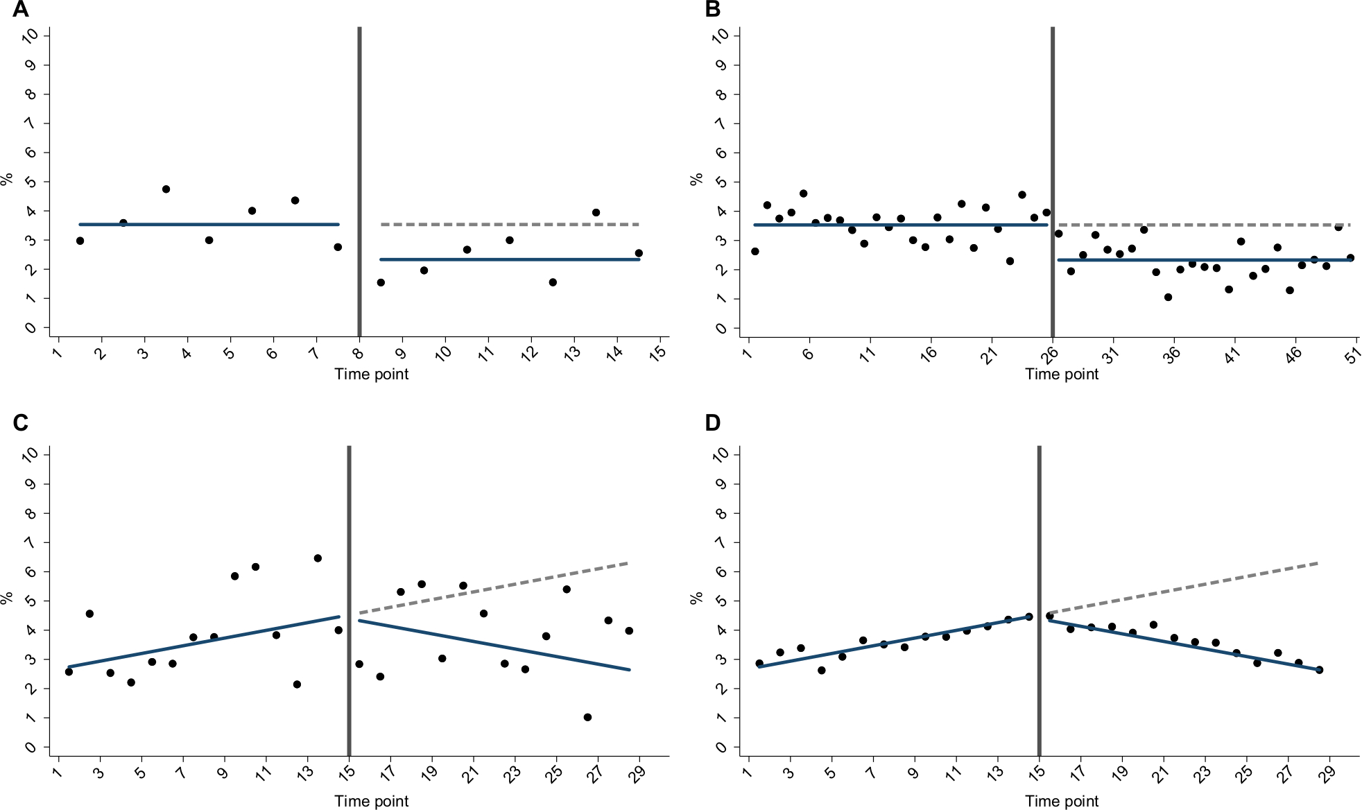Figure 1 Example simulation scenarios for (A) less time points vs (B) more time points; (C) smaller sample size per time point vs (D) larger sample size per time point.

Data-generating process

Data were generated using Stata v15.2 (StataCorp LLC, College Station, TX, USA), the general principles of which have been described elsewhere.²⁴ Empty time series datasets were created of length N (total number of time points). Three ITS variables were inserted: time point identifier (integer), post-intervention indicator (binary), and post-intervention time point identifier (integer).²¹ The time point identifier was created first, then used in combination with the “location of intervention” parameter to generate the other two ITS variables. The underlying sample size for each time point (n_t) was then simulated from a normal distribution with mean n (a key parameter of interest; 11 values investigated) and SD of n/3. The number of outcome events occurring at each time point was then drawn as a binomial random variate (n_t, p_t), where n_t represents the sample size and p_t is the probability of outcome. p_t was a linear function defined using the ITS variables in combination with other scenario-specific parameter values (equation included in the “Supplementary materials” section). The number of events per time point and n_t were used to derive the cumulative incidence time series. A total of 1,000 Monte Carlo repetitions were carried out for each unique scenario.

Methods of analysis

A segmented linear regression model was fitted to each created dataset. This took the form of model (1) for step change scenarios and model (2) for slope change scenarios:

(1)Y_t=β₀ + β₁*time pointt + β₂*intervention_indicatort + e

(2)Y_t=β₀ + β₁*time pointt + β₃*post_intervention_timepointt + e

where Y_t is the value of outcome at time point t. β₀ estimates the level of the outcome just before the beginning of the time series. β₁ estimates the pre-intervention trend, β₂ estimates the change in level between the time point immediately before vs after the intervention, and β₃ estimates the change in trend occurring immediately after the intervention. e is the error term.

Estimands

The target of inference was the change in outcome following a defined intervention, specifically testing the null hypothesis of no change (ie, β₂=0 [model 1] or β₃=0 [model 2]). The outcome at each time point was a proportion, which in our case study was the 5-year cumulative incidence of joint replacement in rheumatoid arthritis patients.²⁰

Performance

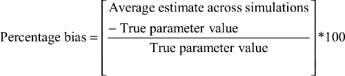
The coefficients, standard error, and P-values from these models were stored, and the empirical power to reject the null hypothesis of no post-intervention change was calculated as the proportion of simulations, where the P-value for the intervention variable coefficient (step/slope change) was <0.05.^19,24,25 This was represented graphically as contour plots across scenarios according to N and n. For the convenience of comparison, additional presentation was made for power according to different effect size and location scenarios while keeping N constant (N=28). In addition, the percentage bias¹⁹ of the regression coefficients was calculated for midway step and slope change scenarios (while keeping N constant), which is defined as follows:

Sensitivity analysis

To explore the impact of pre-intervention level of outcome, we repeated main analyses investigating power for slope and step changes while keeping N constant (N=28) but varying pre-intervention level from 3.5% to 8% and then to 20%.

Stata program

Although we based the current analyses on a case study exploring a range of parameter values adapted from our prior CPRD study as specified earlier,²⁰ we also developed a Stata program (Supplementary materials) with associated documentation (Supplementary materials) to provide a ready-to-use means for assessing power associated with any valid list of (nine) input parameter values as described in the “Supplementary materials” section.

Results

Results from our case study are presented in the following paragraphs describing the impact of N and n on power within several ITS scenarios (Figure 2A and 2B). Results from analyses exploring different effect sizes (whilst keeping N constant) are presented in Figures 3A and 3B. Although the main results pertained to a setting where the mean pre-intervention level of outcome for mid-time series interventions was 3.5%, the Stata program developed can be used to explore alternative input parameter values (Supplementary materials).

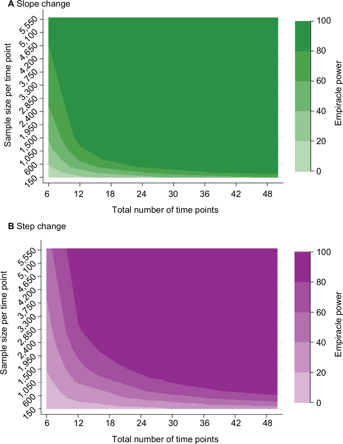Figure 2 Empiracle power to detect a relative 34% reduction in outcome, where mean pre-intervention incidence is 3.5%: by the number of time points and mean sample size per time point: (A) slope change (B) step change.

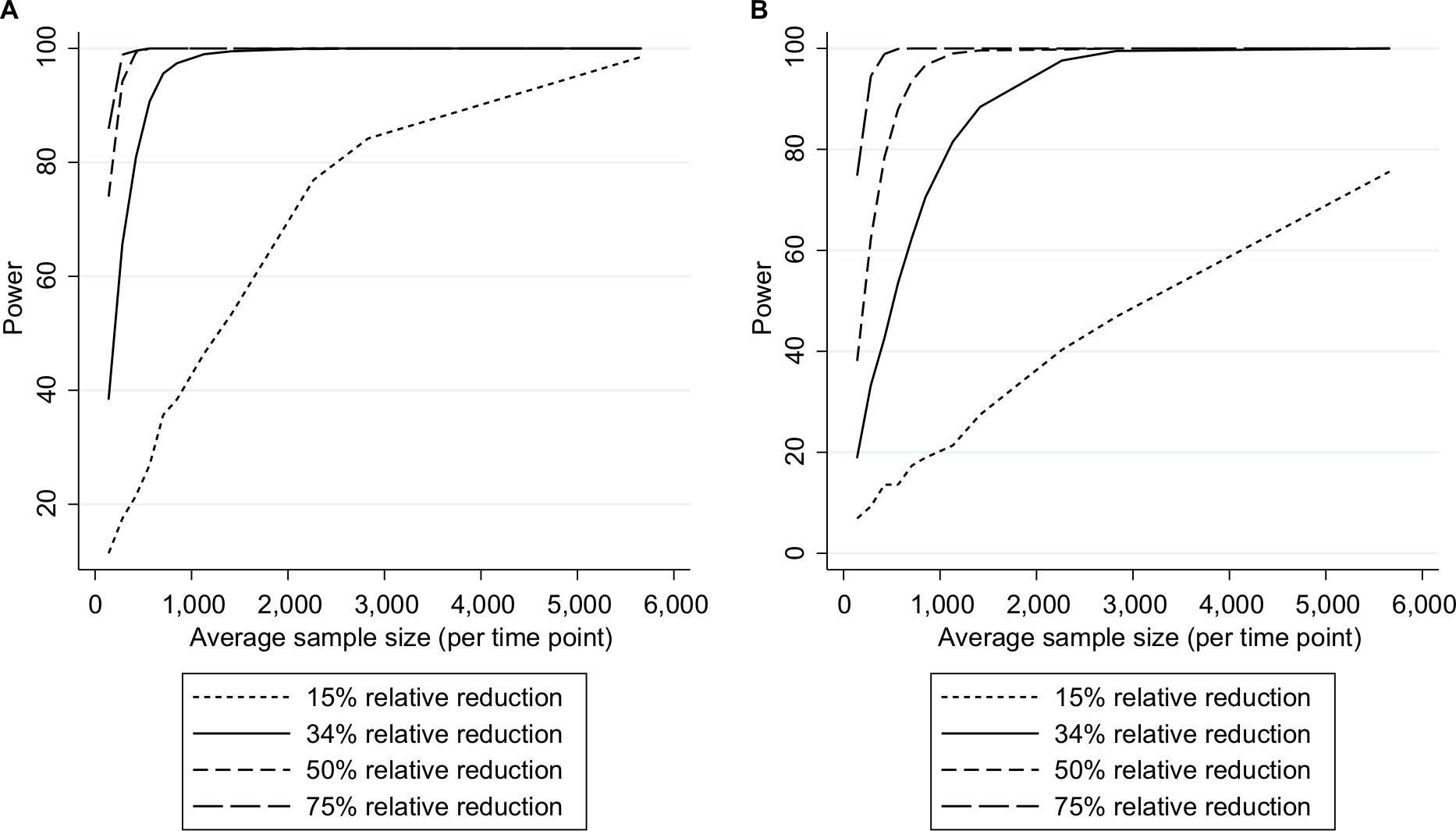Figure 3 Empirical power in the case studya (stratified by effect size) to detect an intervention resulting in (A) a slope change or (B) step change. Note: aAssuming a mean pre-intervention outcome of 3.5%, mid-time series intervention, and 28 total time points.

Slope change

As expected, power increased as N and/or n increased (Figure 2A) and as effect sizes became larger (Figure 3A). Results for different N and n combinations for each effect size investigated are provided in the “Supplementary materials” section. These indicated that nearly all mid-time series intervention scenarios with a large effect size (–75%) had at least 80% power when there were >24 total time points, even when there was a very small sample size per time point (approximately 150 subjects, which in this case-study, corresponded to only five outcome events per time point). However, when the effect size was small (–15%) then to achieve 80% power an analysis had to either contain a large N or very large n (Supplementary materials). While keeping other factors constant (effect size =-34% and N=28), power was greater in scenarios with mid-time series interventions, with comparably less power in scenarios with earlier/later interventions (Figure 4A). The percentage bias in model coefficients was small, and this trended toward zero as sample size increased (Figure 5).

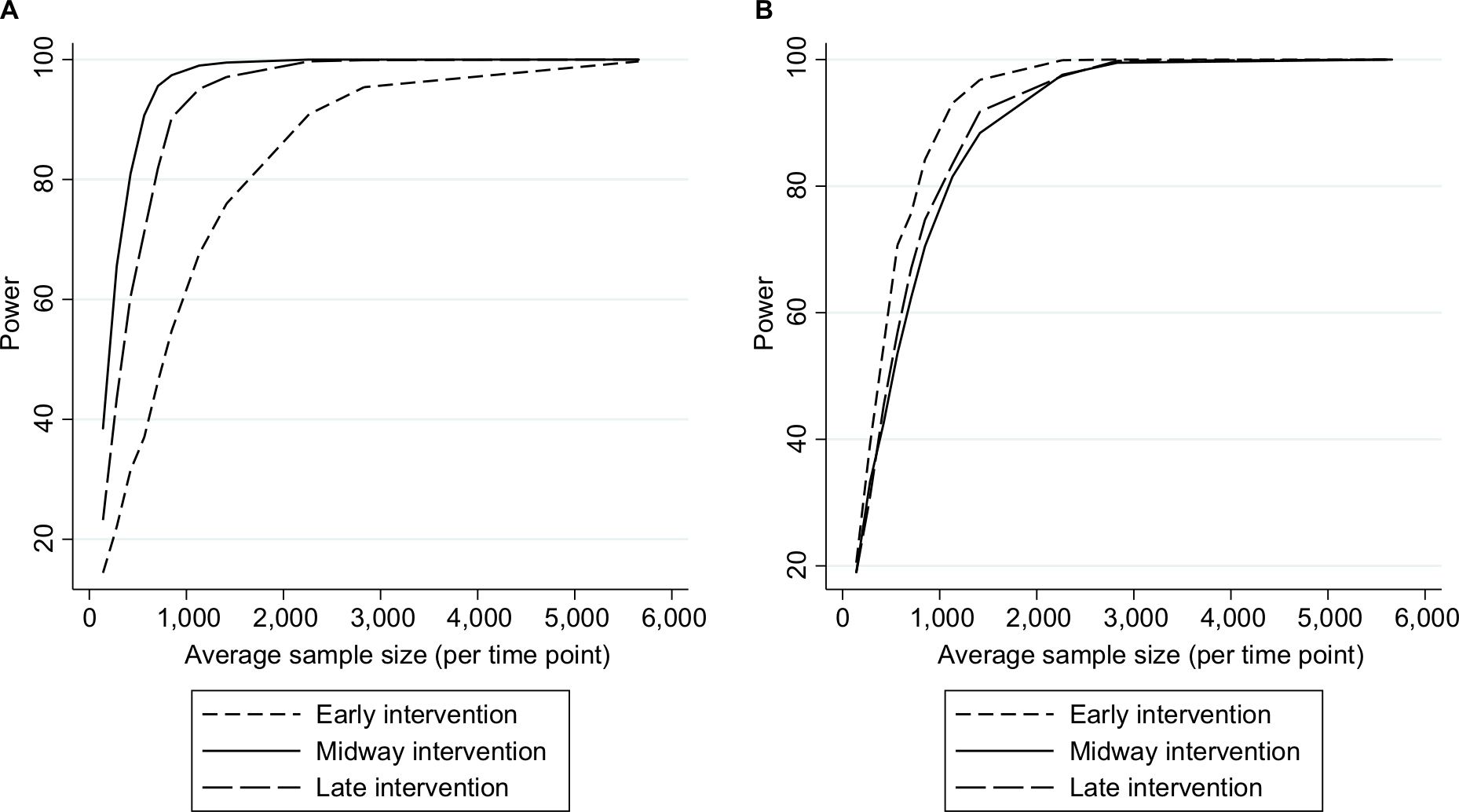Figure 4 Empirical power in the case studya (stratified by intervention location) to detect an intervention resulting in (A) a slope change or (B) step change. Note: aAssuming a mean pre-intervention outcome of 3.5%, 28 total time points, and an average 34% relative reduction post intervention (early/late slope changes were identical to midway scenario, therefore, achieved a different effect size).

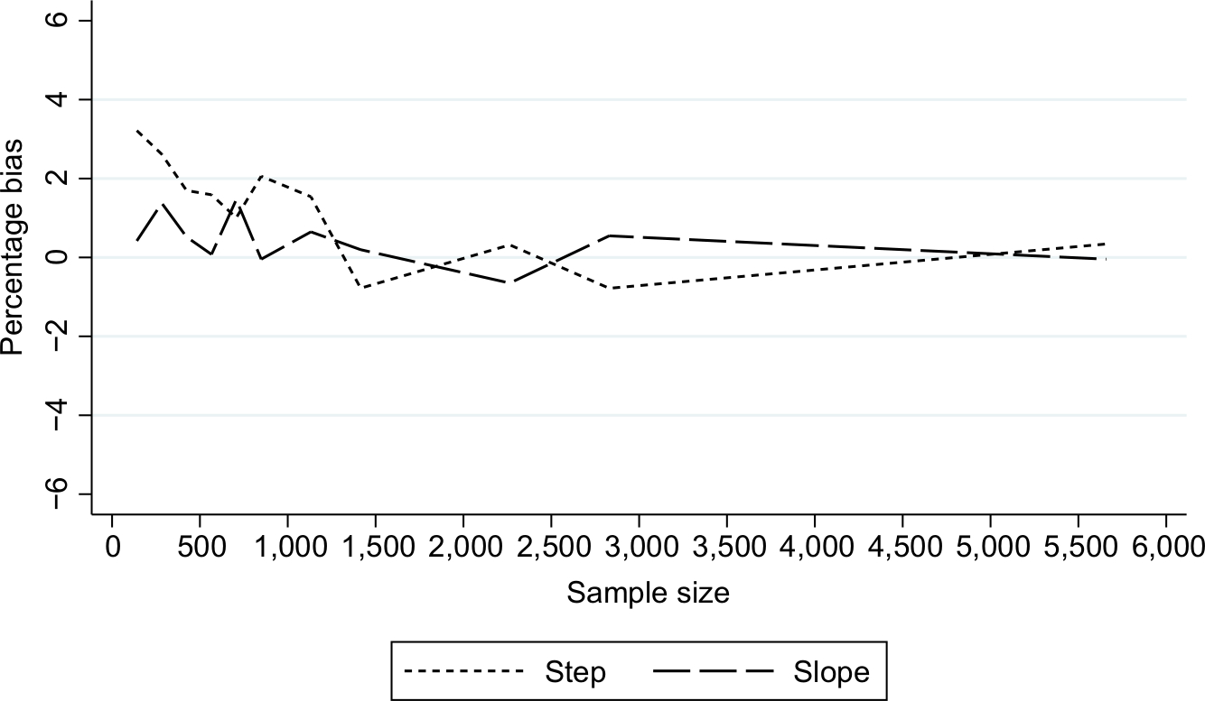Figure 5 Percentage bias in estimates of intervention impact in the case studya: stratified by the nature of impact. Note: aAssuming a mean pre-intervention outcome of 3.5%, total of 28 time points, and an average 34% relative reduction post intervention.

Step change

Similar to slope change scenarios, power increased as N and n became larger (Figure 2B) or as the effect size was larger (Figure 3B). Generally, there was less power in step change scenarios than in corresponding slope change scenarios (Figure 2A and B), with nearly all mid-time series intervention scenarios being inadequately powered when the effect size was only –15% (Figure 3B and Supplementary materials). Even when effect sizes were large and the number of time points was moderate (14 pre-intervention and 14 post-intervention time points), analyses were underpowered if sample size per time point was low (Figure 3B and Supplementary materials). Interestingly, little difference was found in power following an early or late intervention as compared to when the intervention occurred midway through (Figure 4). The percentage bias in model coefficients was small, and this trended toward zero as sample size increased (Figure 5).

Discussion

Main findings

This study demonstrates that simple rules regarding the number of time points are not adequate by themselves to denote an ITS analysis as sufficiently powered. Other factors such as the sample size per time point, expected effect size, location of intervention in the time series, and pre-intervention trends need to be considered. For example, in our case study where mean pre-intervention level of outcome was 3.5%, to achieve 80% power to detect a relative 34% post-intervention step change reduction, with 14 pre- and 14 post-intervention time points, one needed over 1,000 subjects per time point (ie, >28,000 total subjects), which may or may not be realistic for a given study. However, three pre- and post-intervention time points were equally sufficient to achieve 80% power in relatively rare situations of large intervention effect sizes combined with very large sample sizes per time point (Supplementary materials). These results underline the importance of robust pre-study sample size planning. Estimates arising from scenarios with a very small n were only slightly biased, which disappeared as n increased (Figure 3).

That power increases as N increases is an expected finding and has previously been shown for fixed ratios of effect size to the SD of the time series.^10,26 However, we in this study addressed the previously undescribed trade-off between N and n. This is an important consideration and a helpful development. First, the SD of a given number of repeated population-level outcome measures may likely be difficult for applied researchers to estimate in advance of a proposed ITS study. Second, exploring this trade-off between N and n informs to what extent it may be beneficial (in terms of power) when generating an aggregate ITS dataset to sacrifice sample size per time point to increase the number of time points (or vice versa). It allows a combination of N and n to be selected to optimize power. Although the exact nuances of this unique trade-off were scenario specific, in most cases only very little gain in power was achieved when a time series was lengthened at the expense of time point sample size, although gains were more noticeable where a very short time series was lengthened.

To the best of our knowledge, a differential power according to whether an intervention impact is mediated via a slope or step change has not previously been investigated. We found that power was greater in slope change scenarios, a likely explanation being that our effect size was the average difference between post-intervention values and counterfactuals, which in the case of slope change scenarios continued to increase as per the pre-intervention slope and therefore made detection of a change more probable.

Within scenarios with a slope change, we found power to be greater in settings with a balanced number of pre-intervention and post-intervention time points (as opposed to earlier/later interventions), while the location of the intervention had little impact on power to detect step changes and was even marginally greater when the intervention occurred early. Although this was unexpected, it is not without some support from previous work.¹⁰

Limitations

Our study is subject to various limitations. Each time point was a cumulative incidence, and given that individual subjects/patients could only be included in a single time point, we treated time points to be independent. As such, we did not explore what impact autocorrelation may have on estimates, although this remains a subject for further investigation. Despite the availability of ITS approaches that explicitly model autocorrelation, such as autoregressive integrated moving average (ARIMA) models,²⁷ it would seem that where the assumptions of OLS regression are met then this is preferable for epidemiological studies where the goal is likely to be causal inference rather than future prediction. Indeed, while autocorrelation needs to be addressed where present, it has been noted that in epidemiological studies it can often be accounted for by controlling for other variables,² and interestingly of a recent review of over 200 drug utilization studies implementing ITS analysis, 50% were found to use segmented linear regression.¹ Specification of ARIMA models are frequently cited to require a minimum of 50 time points,²⁸ with >100 being preferable,²⁷ yet it is common to have less than this minimum available in epidemiology contexts using routinely collected data.^10,21,23,29 For these reasons, our focus in this study was on “short” time series where we considered 50 time points as a maximum and used Durbin–Watson statistics to confirm that first-order autocorrelation was not present. Previous work investigated the relationship between the number of time points and power in the presence of autocorrelation,^10,30 where positive autocorrelation has been shown to reduce power and negative autocorrelation to increase power.¹⁰ Similarly, we did not consider seasonality nor situations where there may be a delay or waning intervention effect.

Another limitation is that our definition of effect size as the difference between post-intervention time points and counterfactual time points (ie, what would have been observed had pre-intervention level/slope continued uninterrupted) involves extrapolation and therefore uncertainty. While this is often done in practice, with uncertainty of model estimates expressed using CIs,²² there is still the assumption that pre-intervention trends would have continued unchanged.

We only investigated scenarios where the repeated outcome measure is a cumulative incidence (ie, a proportion). This is a common epidemiological measure, but incorporating other common measures such as person-year rates, means (eg, length of hospital stay or drug doses prescribed), and frequencies is a logical next step and remains the subject for imminent further investigation.

Strengths

The disentangling of N and n is a key strength and novel aspect of the current study, as is the separate consideration of post-intervention step and slope changes. Although we did not investigate the impact of varying all of the parameters defined, the development and inclusion of a Stata program are important features of the investigation, facilitating researchers to estimate sample size requirements for future ITS studies in similar applications and thereby promoting the avoidance of carrying out underpowered analyses. We are currently working on using this tool as the basis for an online calculator. It is also worth mentioning that we based the parameter values for our case study on a “real-world” clinical scenario²⁰ to increase the applicability of the findings, rather than starting from arbitrary parameter values.

Conclusion

Multiple factors influence the power of OLS ITS analysis, and these should be collectively taken into account when considering the feasibility of a proposed ITS study. We have demonstrated how a simulation approach can be used to estimate the power available within specific ITS scenarios and provide Stata code to facilitate pre-analysis sample size planning of future ITS studies within similar applications.

Acknowledgments

This study was partially supported by Oxford NIHR Biomedical Research Unit. Andrew Judge was partially supported by the NIHR Biomedical Research Centre at the University Hospitals Bristol NHS Foundation Trust and the University of Bristol. The views expressed in this publication are those of the authors and not necessarily those of the NHS, the National Institute for Health Research, or the Department of Health.

Author contributions

SH, DP-A, and AJ contributed to study conception and design. SH, MSA, and KB contributed to data simulation. SH, KB, and MSA contributed to data analysis. SH contributed to drafting the manuscript. All authors contributed to revising the manuscript critically for important intellectual content, gave final approval of the version to be published, and agree to be accountable for all aspects of the work.

Disclosure

AJ has received consultancy fees from Freshfields Bruckhaus Deringer and is a member of the Data Safety and Monitoring Board (which involved receipt of fees) from Anthera Pharmaceuticals, Inc., outside the submitted work. DP-A’s research group has received unrestricted research grants from Servier Laboratoires, AMGEN, and UCB Pharma. SH, MSA, and KB report no conflicts of interest in this work.

References

1.		Jandoc R, Burden AM, Mamdani M, Lévesque LE, Cadarette SM. Interrupted time series analysis in drug utilization research is increasing: systematic review and recommendations. J Clin Epidemiol. 2015;68(8):950–956.
2.		Lopez Bernal J, Cummins S, Gasparrini A. Interrupted time series regression for the evaluation of public health interventions: a tutorial. Int J Epidemiol. 2017 Feb 1;46(1):348–355.
3.		Ewusie JE, Blondal E, Soobiah C, et al. Methods, applications, interpretations and challenges of interrupted time series (ITS) data: protocol for a scoping review. BMJ Open. 2017;7(6):e016018.
4.		Kontopantelis E, Doran T, Springate DA, Buchan I, Reeves D. Regression based quasi-experimental approach when randomisation is not an option: interrupted time series analysis. BMJ. 2015;350:h2750.
5.		Hawton K, Bergen H, Simkin S, et al. Long term effect of reduced pack sizes of paracetamol on poisoning deaths and liver transplant activity in England and Wales: interrupted time series analyses. BMJ. 2013;346:f403.
6.		Laliotis I, Ioannidis JPA, Stavropoulou C. Total and cause-specific mortality before and after the onset of the Greek economic crisis: an interrupted time-series analysis. Lancet Public Health. 2016;1(2): e56–e65.
7.		Craig P, Cooper C, Gunnell D, et al. Using natural experiments to evaluate population health interventions: new Medical Research Council guidance. J Epidemiol Community Health. 2012;66(12):1182–1186.
8.		Lenth RV. Some practical guidelines for effective sample size determination. Am Stat. 2001;55(3):187–193.
9.		Ramsay CR, Matowe L, Grilli R, Grimshaw JM, Thomas RE. Interrupted time series designs in health technology assessment: lessons from two systematic reviews of behavior change strategies. Int J Technol Assess Health Care. 2003;19(4):613–623.
10.		Zhang F, Wagner AK, Ross-Degnan D. Simulation-based power calculation for designing interrupted time series analyses of health policy interventions. J Clin Epidemiol. 2011;64(11):1252–1261.
11.		Fretheim A, Zhang F, Ross-Degnan D, et al. A reanalysis of cluster randomized trials showed interrupted time-series studies were valuable in health system evaluation. J Clin Epidemiol. 2015;68(3):324–333.
12.		Penfold RB, Zhang F. Use of interrupted time series analysis in evaluating health care quality improvements. Acad Pediatr. 2013;13(6 Suppl):S38–S44.
13.		Cordtz RL, Hawley S, Prieto-Alhambra D, et al. Incidence of hip and knee replacement in patients with rheumatoid arthritis following the introduction of biological DMARDs: an interrupted time-series analysis using nationwide Danish healthcare registers. Ann Rheum Dis. 2018;77(5):684–689.
14.		Van Calster B, Steyerberg EW, Collins GS, Smits T. Consequences of relying on statistical significance: Some illustrations. Eur J Clin Invest. 2018;48(5):e12912.
15.		Button KS, Ioannidis JP, Mokrysz C, et al. Power failure: why small sample size undermines the reliability of neuroscience. Nat Rev Neurosci. 2013;14(5):365–376.
16.		Chang M. Monte Carlo Simulation for the Pharmaceutical Industry: Concepts, Algorithms, and Case Studies. Boca Raton: CRC Press; 2010.
17.		Ripley BD. Stochastic Simulation. New York, USA: John Wiley and Sons Ltd; 2006.
18.		Morris T, White I, Crowther M. Using simulation studies to evaluate statistical methods. Tutorial in Biostatistics. 2017.
19.		Burton A, Altman DG, Royston P, Holder RL. The design of simulation studies in medical statistics. Stat Med. 2006;25(24):4279–4292.
20.		Hawley S, Cordtz R, Dreyer L, Edwards CJ, Arden NK, Delmestri A, Cooper C, Judge A, Prieto-Alhambra D. The Impact of Biologic Therapy Introduction on Hip and Knee Replacement Among Rheumatoid Arthritis Patients: An Interrupted Time Series Analysis Using the Clinical Practice Research Datalink [Abstract]. Arthritis Rheumatol. 2016;68(suppl 10).
21.		Wagner AK, Soumerai SB, Zhang F, Ross-Degnan D. Segmented regression analysis of interrupted time series studies in medication use research. J Clin Pharm Ther. 2002;27(4):299–309.
22.		Zhang F, Wagner AK, Soumerai SB, Ross-Degnan D. Methods for estimating confidence intervals in interrupted time series analyses of health interventions. J Clin Epidemiol. 2009;62(2):143–148.
23.		Hawton K, Bergen H, Simkin S, et al. Effect of withdrawal of co-proxamol on prescribing and deaths from drug poisoning in England and Wales: time series analysis. BMJ. 2009;338:b2270.
24.		Feiveson AH. Power by simulation. Stata J. 2002;2(2):107–124.
25.		Sayers A, Crowther MJ, Judge A, Whitehouse MR, Blom AW. Determining the sample size required to establish whether a medical device is non-inferior to an external benchmark. BMJ Open. 2017;7(8):e015397.
26.		McLeod AI, Vingilis ER. Power computations in time series analyses for traffic safety interventions. Accid Anal Prev. 2008;40(3):1244–1248.
27.		Box GEP, Jenkins GM, Reinsel GC, Ljung GM. Time Series Analysis: Forecasting and Control. 5th ed. Hoboken, NJ: Wiley; 2015.
28.		Chatfield C. The Analysis of Time Series: An Introduction. Chatfield CTM, Zidek J, editors. Taylor & Francis e-Library: CHAPMAN & HALL/CRC; Boca Raton, Florida. 2004.
29.		Hawley S, Leal J, Delmestri A, et al; REFReSH Study Group. Anti-Osteoporosis Medication Prescriptions and Incidence of Subsequent Fracture Among Primary Hip Fracture Patients in England and Wales: An Interrupted Time-Series Analysis. J Bone Miner Res. 2016;31(11):2008–2015.
30.		McLeod AI, Vingilis ER. Power Computations for Intervention Analysis. Technometrics. 2005;47(2):174–181.