Regression Discontinuity Designs in Epidemiology: A Practical Guide

Introduction

Clinical epidemiological research studies often involve the use of observational data to answer questions concerning the effect of a treatment or intervention on a clinical outcome of interest. However, many such studies are often hampered by confounding, in particular, confounding by indication. For example, in observational studies evaluating the effectiveness of a new antihypertensive drug, patients who are prescribed the drug may have more severe hypertension or additional comorbidities compared to those who are not treated. As a result, worse outcomes observed in the treated group may reflect the underlying severity of illness rather than the effect of the drug itself, thereby confounding the interpretation of the drug’s effectiveness.

Yet, there may be ways to overcome this issue in certain situations because some clinical treatments or interventions are administered according to external rules based on individual-level variables or data. For example, the UK’s National Institute for Health and Care Excellence (NICE) has devised many evidence-based treatment/intervention rules including:

(i) Statins (a class of cholesterol-lowering drugs) are recommended for people with a 10-year cardiovascular disease (CVD) risk score ≥10%,¹ where 10-year CVD risk is calculated using data from individuals’ electronic health records (eg QRISK3);²

(ii) Corticosteroid replacement is recommended for people with suspected adrenal insufficiency, whose serum cortisol level is measured to be below 150nmol/L;³

(iii) Referral to local, evidence-based, quality-assured intensive lifestyle-change programme is recommended for people at risk of Type 2 diabetes whose HbA1c level is measured to be >42mmol/mol.⁴

Each of these is a clinical “decision rule” based on an “assignment variable” (or “running variable”), where a “threshold” separates the “treated” from the “untreated”. For example, in (i), the 10-year CVD risk score of 10% is a “threshold” and a person whose 10-year CVD risk score is at or above 10% is recommended to receive a statin prescription, whereas a person whose 10-year CVD risk score is below 10% is not recommended to receive a statin prescription.¹

Because such decision rules are externally defined (and therefore not influenced by variability between individuals) we can consider groups of individuals whose assignment variable values are “just above” the threshold and individuals whose assignment variable values are “just below” the threshold to be from the same population. As a result, we might assume that these individuals share similar characteristics and – crucially – are generally similar with respect to potential confounding variables for the treatment-outcome association.

The regression discontinuity design (RDD) is a method for causal treatment/intervention effect estimation that exploits the threshold-based treatment rule.⁵ A key idea is that, within a small region close to the threshold, the two groups of individuals: (a) with assignment variable values “just above” the threshold; (b) with assignment variable values “just below” the threshold are considered balanced with respect to potential confounding variables. As such, these groups might be seen as similar to the randomised groups in a two-group individually randomised controlled trial (RCT), with the threshold acting as a quasi-randomising device – similar to a randomising device, but in an observational, rather than an experimental, setting. Therefore, if one group (eg individuals above the threshold) receives the treatment/intervention according to the decision rule but the other (eg individuals below the threshold) does not – and the groups are balanced with respect to potential confounding variables – then a valid comparison of an outcome of interest between these groups can provide a causal treatment/intervention effect estimate at the threshold. RDDs have been used extensively in economics, sociology and politics^6–8 and, although RDDs have been under-used in epidemiology in the past,⁹ applications to epidemiological data and clinical questions of interest are increasing.¹⁰

The use of RDDs in clinical epidemiology is less common than other quasi-experimental approaches. This is possibly because treatment/intervention assignment can often be more variable than a strict decision-based guideline, even when such a guideline exists, and this could lead to potential users assuming that an RDD is not suitable for a given dataset. In addition, until recently, there has been limited statistical software for RDDs which may have restricted use by applied researchers.

With this in mind, the main aim of this paper is to provide an overview of the RDD, with particular emphasis on how it can be used in clinical epidemiology. Our specific aims are to: (i) describe the key concepts of an RDD; (ii) outline necessary assumptions for RDD use in clinical epidemiology, together with a guide on how these can be assessed; (iii) describe how continuity-based and local randomisation RDDs can be fitted to epidemiological data, using informative examples; (iv) discuss how treatment/intervention effects from RDDs can be interpreted.

Overview of the RDD

We consider a scenario where, for each of a group of individuals, a continuous “assignment variable” (sometimes known as a “running variable”) is measured. This variable is then compared to a pre-defined, external, threshold that is used to determine treatment, where:

• An individual should receive the treatment/intervention if their assignment variable value is at or above the threshold.
• An individual should not receive the treatment/intervention if their assignment variable value is below the threshold.

As an example, as noted previously, in the UK, NICE recommends that statins (a class of cholesterol-lowering drugs) should be prescribed to people with a 10-year cardiovascular disease (CVD) risk score ≥10%.¹ Here, a sample from a population of interest would be chosen and a 10-year CVD risk score calculated for each sampled individual. The risk score would then be compared to the 10% threshold, and if the risk score is ≥10%, the individual would be recommended to receive statins. Conversely, if the risk score is <10%, the individual would not be recommended to be prescribed statins. Statins are designed to reduce LDL cholesterol and, hence, the outcome of interest is an individual’s LDL cholesterol level (in mmol/L) at some point of interest (eg three months after the measurement of the 10-year CVD risk score, to allow statins, where prescribed, to affect the LDL cholesterol level).

Sharp RDD

Suppose that the threshold decision rule is followed strictly for all individuals. Figure 1 shows an example plot of how data might look in the 10-year CVD risk score example, described previously, under this scenario. This is known as a “sharp RDD” – where the threshold is a strict separator for the “treated” (above threshold) and “untreated” (below threshold) groups.

Figure 1 Scatter plot showing the post-decision LDL cholesterol – 10-year CVD risk score relationship in a sharp RDD. All individuals with risk scores below the threshold do not receive statins and all individuals with risk scores above the threshold receive statins. A + symbol denotes an individual that receives statins, a ○ symbol denotes an individual that does not receive statins.

Fuzzy RDD

In many situations, sharp RDDs are not applicable – especially in clinical epidemiology. This is because an external treatment/intervention decision rule might not be followed strictly for all individuals, often for a number of different reasons. For example, in the 10-year CVD risk score for statin prescription example, it might be that a clinician thinks that an individual might benefit from statins, even if their 10-year CVD risk score is below the threshold. Or, an individual might request statins, even if their 10-year CVD risk score does not entitle them to a prescription, according to the decision rule. Conversely, individuals with risk scores above the threshold might prefer to reduce their LDL cholesterol using dietary or lifestyle choices, rather than by taking statins. As a result, we might have a scenario where, for some individuals, the decision rule is not followed strictly. This is known as a “fuzzy RDD”, with fuzziness occurring because of non-adherence to the decision rule for some individuals. Figure 2 shows a plot of how data might look in the 10-year CVD risk score example, where there is some fuzziness with respect to the threshold decision rule.

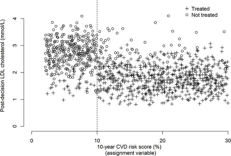Figure 2 Scatter plot showing the post-decision LDL cholesterol – 10-year CVD risk score relationship in a fuzzy RDD. Some individuals with risk scores below the threshold receive statins and some individuals with risk scores above the threshold do not receive statins. A + symbol denotes an individual that receives statins, a ○ symbol denotes an individual that does not receive statins.

In Figure 2, we see that there are some individuals whose 10-year CVD risk score is above 10%, but they did not receive statins. Conversely, there are some individuals who received statins, despite their 10-year CVD risk score being below 10%. In this scenario, the threshold does not strictly separate the “treated” and “untreated”. However, this does not mean that an RDD cannot be used to estimate the treatment effect at the threshold. In fact, fuzzy RDDs are common and, as we will see, can be easily applied – subject to certain assumptions being valid.

We now focus on important data properties and assumptions that should hold for an RDD to be valid. We concentrate on fuzzy RDDs, because these are encountered most often in practice, but we note that all materials are valid for a, simpler, sharp RDD.

RDD Key Concepts

First, we have noted that the RDD relies on groups of individuals whose assignment variable values lie “just above” the threshold and “just below” the threshold and considers these groups to be balanced with respect to potential confounding variables. In the 10-year CVD risk score for statin prescription example, we can easily imagine that a group of individuals with 10-year CVD risk scores close to 30% might be very different from a group of individuals with 10-year CVD risk scores close to 5% - perhaps with respect to important features such as age, body mass index, smoking status etc. An assumption that these groups are balanced with respect to such variables is not likely to hold. On the other hand, around the 10% threshold, we might consider that individuals with risk scores above the threshold, close to 11%, as similar to individuals with risk scores below the threshold and close to 9%. Consequently, we note that an RDD treatment/intervention effect estimate is an effect “at the threshold” and applies only to those individuals in a region around the threshold. The region around the threshold is quantified by defining a “window” or “bandwidth”.

Suppose that we have a sample of individuals and is the individual’s assignment variable. If denotes the threshold, and the decision rule is defined:

“The individual should receive the treatment/intervention if ”, then a “window” or “bandwidth”, , is chosen and we would only include data from the individual in the RDD if their assignment variable lies within of the threshold (ie if ). We will discuss the choice of a window later.

In the 10-year CVD risk score for statin prescription example, we have individual’s 10-year CVD risk score and 10%.

Assumptions

For an RDD to be valid as a method to estimate a treatment/intervention effect at the threshold, we require specific assumptions to hold in a region around the threshold – defined by the RDD window. We outline these briefly and explain how they might be assessed.

Assumption 1

The probability of receiving the treatment/intervention should differ for individuals with assignment variables above the threshold and individuals below the threshold. In a sharp RDD, we know that the probability of receiving the treatment/intervention is 1 on one side of the threshold and 0 on the other, because all individuals who meet the threshold receive the treatment, whereas those who do not will not receive the treatment (depending on the direction of the decision rule). For a fuzzy RDD, there should be allocation to the treatment/intervention more often on one side of the threshold, compared to the other. To assess this, we might produce a plot of the probability of treatment – calculated for subgroups of individuals (ranked by the assignment variable) – against the assignment variable. Figure 3 shows an example plot for the 10-year CVD risk – statin prescription example.

Figure 3 Example plot showing empirical estimates of the probability of being prescribed statins, by risk score group. Risk scores were grouped into bins containing equal numbers of individuals, and the proportion of individuals who receive statins calculated for each bin.

In Figure 3 it is clear that there is a discontinuity at the threshold with respect to the probability of treatment. For an RDD to be valid, we should expect to see a plot similar to that in Figure 3, where the probability of receiving the treatment/intervention differs substantially on either side of the threshold. If we do not see a discontinuity at the threshold, we cannot apply the RDD design. We also assume that an individual cannot manipulate their own assignment variable in an effort to place them above (or below) the threshold and then receive (or not receive) the treatment/intervention.

Assumption 2

It is not the threshold itself that affects an outcome of interest (ie being above/below the threshold itself does not cause a change in an outcome). Instead, it is the relationship between the threshold and treatment/intervention assignment and then the treatment/intervention itself that might affect the outcome. In other words, any change in the outcome variable at the threshold occurs because of the treatment/intervention. This assumption is not testable, however, in many examples, we can justify its use. As a result, we should expect that – if an individual’s treatment allocation is always held fixed (irrespective of their assignment variable value) then we would not expect to see a change in their outcome of interest at the threshold. This is because, for a given individual, only a change in their treatment allocation should cause an effect on the outcome at the threshold.

In conjunction with this assumption, and for the RDDs considered in this paper, it is assumed that only one decision rule occurs in relation to the threshold. In other words, it is not the case that there is another decision rule linked to the same assignment variable or that multiple treatments/interventions might be allocated at the threshold.

Assumption 3

Around the threshold (ie in the region defined by the RDD window), groups either side of the threshold have similar distributions of potential confounding variables. This means that, within this region, individuals should not be more (or less) likely to be placed on one side of the threshold. In other words, close to the threshold, we assume that individuals occur randomly on either side of the threshold, with respect to their assignment variable. This assumption implies that we consider the threshold to be a quasi-randomising device and that groups either side of the threshold can viewed as similar to randomised groups in a two-group individually randomised RCT.

To assess this assumption, once the RDD window is chosen, summaries of known potential confounding variables can be produced, separately for groups above and below the threshold, to compare the distributions. Formal comparisons between groups above/below the threshold, such as appropriate hypothesis tests (eg t-tests, Pearson chi-squared tests or Mann–Whitney U-tests) can be made with respect to confounding variables, to demonstrate that there is balance between groups. Although useful in practice, this does not always guarantee that confounding variables are similarly distributed above and below the threshold.

Assumption 4

If the RDD is fuzzy, we assume that there are no practitioners (ie those responsible for delivering the treatment/intervention) who would always allocate treatment in the opposite way to the decision rule. For example, in the 10-year CVD risk score example, we should assume that there are no practitioners who would always prescribe statins to individuals with 10-year CVD risk scores below 10% and never prescribe stations to individuals with 10-year CVD risk scores at or above 10%. If a dataset contains a record of the person responsible for making the treatment decision rule (we term this a “prescriber”), then this assumption can be explored by examining summaries of each prescriber’s decisions for individuals above and below the threshold.

Estimating the Treatment/Intervention Effect

In an RDD, the treatment/intervention effect estimate is a “local” estimate, in that it is an effect estimate at the threshold and applies only to those whose assignment variable lies close to the threshold (with the concept of “close to” defined by the RDD window).

For a sample of n individuals, we assume that is the outcome of interest. For example, in the 10-year CVD risk – statin prescription scenario that we described earlier, would be the individual’s LDL cholesterol measurement, three months after their 10-year CVD risk score was measured. We will assume that is continuous, but we note that RDD extensions exist for cases where is discrete or a time-to-event.^11,12

Potential Outcomes

With respect to the outcome , we define the pair of “potential outcomes” ) and ), where ) is the outcome that would occur if the individual does not receive the treatment/intervention and ) is the outcome that would occur if the individual receives the treatment/intervention. At the individual level, the treatment effect on the outcome can be defined as the difference in means of the potential outcomes. That is,

However, this definition applies only in theory because, for a given individual,) and ) cannot both be observed. This is because an individual cannot be both “treated” and “not treated”. In practice, we define as a treatment indicator, where if the individual is treated and if not. Then, the actual outcome (ie the outcome that we will observe for the individual) is

Estimand at the Threshold

As noted previously, an RDD aims to estimate a local treatment/intervention effect. In other words, an effect estimate at the threshold that will be formed using data from individuals with assignment variable values within a small window around the threshold.

For an RDD, the estimand (ie the measure that we want to estimate) is the local average treatment effect (LATE) at the threshold. In this case, the LATE measures the effect of the treatment/intervention at the threshold for those individuals who would comply with the treatment/intervention if assigned to them. The RDD LATE is similar to the complier average causal effect (CACE), used routinely as an intervention effect estimate for “compliers” in RCTs. Here, the term “comply” means that the individual would follow the treatment/intervention programme. For example, they would take all prescribed medication, or attend all intervention sessions (eg therapy or counselling) as directed. This estimand differs from the “average treatment effect” (ATE) at the threshold which compares those allocated to receive the treatment/intervention to those not allocated the treatment/intervention, irrespective of whether or not an individual actually takes/complies with the treatment/intervention. The ATE estimate can be viewed as similar to an “intention to treat” (ITT) estimate in an RCT. Further technical detail on LATE estimation can be found in Imbens et al¹³ and Hahn et al.¹⁴

In an RDD, the threshold is used as a randomising device and, for each individual, we define the binary variable as a “threshold indicator” where

The estimand at the threshold is then

where

Mean of the outcome variable for those “just above” the threshold;

Mean of the outcome variable for those “just below” the threshold;

Probability of receiving the treatment/intervention for those “just above” the threshold;

Probability of receiving the treatment/intervention for those “just below” the threshold.

As noted previously, the terms “above” and “below” the threshold are with respect to the assignment variable. This estimand is valid for both fuzzy and for sharp RDDs. In a sharp RDD, and because all individuals with assignment variable values above the threshold are treated and those with variables below the threshold are not. In a fuzzy RDD, the LATE denominator adjusts for the fuzziness of the design and ensures that the LATE estimator estimates the causal effect of the treatment/intervention at the threshold.

We now turn our attention to how to estimate the LATE in an RDD. We focus on the common case where the outcome of interest is continuous – some extensions are noted in the Discussion section. There are two main methods that are used for estimation in an RDD: (i) Continuity-based estimation, (ii) Local randomisation-based estimation. Both approaches can be fitted easily using standard statistical software (eg R or Stata). We will outline both methods briefly before describing their use in an example.

Estimation Methods

Continuity-Based Estimation

The continuity-based method for RDD uses flexible models for the relationship between the assignment variable and outcome, separately on each side of the threshold. The idea is that these models capture a realistic relationship between the assignment variable and outcome and account for any fuzziness present in the RDD, so that the LATE at the threshold is estimated precisely and in an unbiased way.

When fitting a continuity-based RDD using standard statistical software, the window (or bandwidth) around the threshold is selected automatically. This selection is done to ensure that the estimate of the LATE is unbiased and precise (subject to RDD assumptions being valid). Further details on the theory can be found in^14–16

Models for the outcome and for treatment are fitted. These are defined:

(model for the outcome where is at/above the threshold);

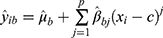(model for the outcome where is below the threshold);

(model for the treatment indicator where is at/above the threshold);

(model for the treatment indicator where is below the threshold).

These models are flexible because they may have many terms in powers of . This means that the relationship between the assignment and outcome (or treatment) can vary in shape to fit with the data. To fit a continuity-based RDD we must specify an order, , where is the highest power of . Essentially, , controls the form of the relationship between the assignment variable and outcome. For higher values of , the relationship between the variables is more flexible (ie there may be a curved relationship with lot of turning points) whereas if is small, models for the relationship between variables are less flexible. For example, if then the relationships between the outcome and assignment variable are straight lines because

The order () should be chosen to reflect the relationship between the outcome and assignment variable. Often, an exploratory plot of the assignment variable against the outcome can help as a visual assessment for the relationship between and . Typically, smaller order models are often preferred because of their simplicity.

As an example, Figure 4 shows a plot of some simulated RDD data from a fuzzy RDD, where the threshold is and the treatment effect at the threshold is 2. The data have been simulated so that there is a quadratic relationship between the outcome variable, , and the assignment variable, . We can fit a continuity-based fuzzy RDD to model these data using R or Stata.

Figure 4 Scatter plot of the outcome against the assignment variable with icons to distinguish between treated and non-treated individuals. A + symbol denotes an individual that receives treatment, a ○ symbol denotes an individual that does not receive treatment. The dashed line shows the threshold, where the assignment variable = 0.5.

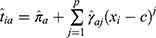
In R, we use the package rdrobust.¹⁷ R code to fit the RDD is provided in the supplementary material that accompanies this paper and the corresponding R output is shown in Figure 5. Key measures in Figure 5 are highlighted in yellow as follows:

Figure 5 R output from fitting a continuity-based RDD to the simulated data shown in Figure 4.

“BW est. (h)”: This shows the chosen window (or bandwidth, ). Here .

“Eff. Number of Obs.”: This shows the numbers of data points within of the threshold. Here, within the window, there are 215 individuals with assignment variable values below the threshold and 243 individuals with assignment variable values above the threshold.

“Treatment effect estimates.”: This table shows the treatment effect estimate at the threshold. Here, the estimate is 1.994 with standard error 0.409. Also shown are two 95% confidence intervals for the treatment effect – the first is a standard 95% confidence interval: (1.193, 2.796) and the second is a robust 95% confidence interval: (1.135, 2.954). Often, it is good practice to report the robust 95% confidence interval because this accounts for any bias in having estimated the treatment effect at the threshold using a fuzzy RDD. For a sharp RDD, the standard and robust 95% confidence intervals would be the same.

The same RDD can also be fitted using Stata, using the rdrobust command.¹⁸ Full Stata commands to fit the RDD are provided in the supplementary material and the corresponding Stata output is shown in Figure 6.

Figure 6 Stata output from fitting a continuity-based RDD to the simulated data shown in Figure 4.

The continuity-based RDD is flexible, data-driven, easy to fit and results in valid inference (subject to the accuracy of RDD assumptions). It is particularly useful in scenarios when an RDD setting does not necessarily emulate an RCT directly. For example, a treatment programme might vary either side of a health care trust geographical boundary and individuals who live close to (but either side) of the boundary may be subject to different treatment programmes/regimes for a disease. An RCT would not be used to determine treatment efficacy because the “threshold” occurs naturally. A continuity-based RDD might be helpful in exploiting the geographical quasi-randomising device to investigate the differing effects of the treatment programmes.

Where an RDD is analogous to an RCT (eg where a specific patient-based rule is used to determine treatment/intervention allocation) and, in a region close to the threshold, groups either side are assumed to be balanced with respect to potential confounding variables, a local randomisation RDD can be used to estimate the treatment/intervention effect at the threshold.

Local Randomisation RDD Estimation

In a local randomisation RDD, the window (or bandwidth) is pre-selected before fitting any models. When pre-selecting the window, the aim is to choose as wide a window as possible around the threshold such that the groups either side of the threshold are balanced with respect to potential confounding variables. In this way, we seek groups either side of the threshold that are similar to the two groups in an individually randomised controlled trial, but with the threshold as a quasi-randomisation device in an observational setting, rather than true randomisation as would occur in an experimental setting. Selection of the window might involve extensive discussions between clinicians, epidemiologists, health care researchers and statisticians to ensure that the chosen groups are balanced. In addition, where data are available on potential confounding variables, groups can be compared formally using tests of the null hypothesis of no difference between groups with respect to a given confounding variable. In carrying out these tests, we would seek to retain, rather than reject, the null hypothesis so that there is evidence in favour of balance between groups.

Once the window is selected, groups either side of the threshold are assumed to be balanced with respect to confounding variables, and a simpler two-stage least squares model is fitted to estimate the treatment effect at the threshold. The two-stage least squares method ensures that fuzziness, where present, is accounted for.

We can fit a local randomisation RDD to model the data from Figure 4 using R or Stata. For this demonstrative example, we assume that the window/bandwidth is – so an individual is included in the RDD if their assignment variable is in the range 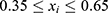. In the section “Example: Prescription of Statins According to 10-year CVD Risk Score”, we include a local randomisation example with observed confounding variables and use hypothesis tests to justify the window choice.

To fit the local randomisation RDD in R, we use the rdlocrand package,¹⁹ R code to fit the local randomisation RDD is provided in the supplementary material, and the corresponding R output is shown in Figure 7. Key measures in Figure 7 are highlighted in yellow as follows:

Figure 7 R output from fitting a local randomisation RDD, with window 0.35 to 0.65, to the simulated data shown in Figure 4.

“Eff. number of obs” shows the number of data points used above and below the threshold. In this example, within the specified window, 153 individuals have assignment variables below the threshold, and 166 individuals have assignment variables above the threshold.

“TSLS” shows the estimate of the treatment effect at the threshold, here this is estimated as 2.005. A 95% confidence interval for the treatment effect at the threshold is (1.76, 2.25).

The same model can be fitted using Stata, by installing the rdlocrand package.²⁰ Stata commands to fit the RDD are provided in the supplementary material, and the corresponding Stata output is shown in Figure 8.

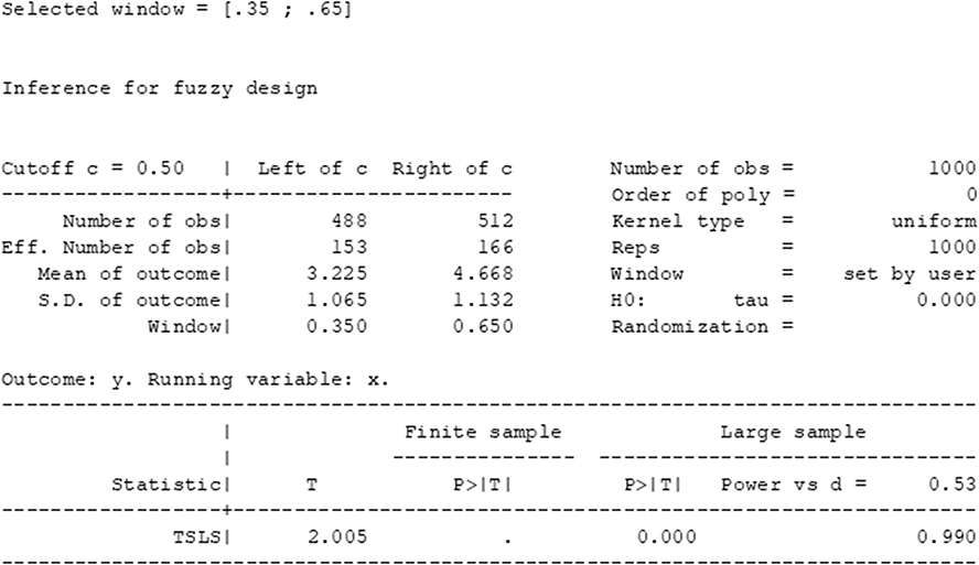Figure 8 Stata output from fitting a local randomisation RDD, with window 0.35 to 0.65, to the simulated data shown in Figure 4.

To obtain precise estimates of the treatment/intervention effect, it is important that – once a method is selected – the sample size (ie the number of individuals whose assignment variables lie within the bandwidth or window) is sufficient. Sample size calculation is not straightforward, as this depends on many variables, including the fuzziness of the design, the strength of the treatment/intervention effect at the threshold, the window/bandwidth which is, in turn, related to features such as bias and confounding. RDDs, by nature, are often retrospective, especially in clinical epidemiology where randomised trials and other evidence-based approaches may have been used to determine the decision rule prior to its application. Some guidance for the continuity-based approach is provided in Cattaneo et al.²¹ Generally, for either approach, we would recommend examining measures of precision, such as 95% confidence interval widths or standard error estimates, to ensure that estimates are precise.

These examples have presented a basic RDD without any additional variables. In the next section, we present examples based on the 10-year CVD risk score – statin prescription rule, described earlier.

Example: Prescription of Statins According to 10-Year CVD Risk Score

As discussed previously, in the United Kingdom, the National Institute for Health and Care Excellence (NICE) has a guideline in place regarding the prescription of statins for the primary prevention of cardiovascular disease. The guideline states that an individual with a 10-year CVD risk score of 10% or more should be prescribed statins, a class of cholesterol-reducing oral drugs. An individual’s 10-year CVD risk score is an estimate of the probability that the individual will experience a CVD event (eg a stroke or myocardial infarction) within 10 years. Typically, an individual’s 10-year CVD risk score is calculated by their general practitioner (GP) using a validated risk prediction scoring algorithm, such as the QRISK3 score.^1,2 Statins are a class of cholesterol-lowering drugs and, therefore, we aim to use an RDD based on the above decision rule, to estimate the effect of statins on low density lipoprotein (LDL) cholesterol. The assignment variable is the 10-year CVD risk score, the threshold is a 10-year CVD risk score of 10% and the outcome of interest is the LDL cholesterol level at least three months after the 10-year CVD risk score measurement was made.

In this example, we use a simulated dataset containing data that represent 2000 males, aged between 55 and 75 years who had not previously been prescribed statins. The simulated dataset is based closely on a smaller, real data sample from electronic primary care health records.²² We use an RDD to estimate the effect of statins on LDL cholesterol level, with a dataset that contains, for each individual, their:

• 10-year CVD risk score (ie the assignment variable);
• LDL cholesterol measurement (mmol/L) at least three months after the 10-year CVD risk score measurement (ie the outcome variable);
• LDL cholesterol measurement at the time of the 10-year CVD risk score measurement;
• Systolic and diastolic blood pressure;
• Age (years);
• Smoking status (a binary variable = 1 if the individual is a current smoker; = 0 if not).

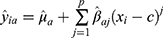
Before using an RDD, we produce a scatterplot of the 10-year CVD risk score against the outcome (ie the LDL cholesterol measurement at least three months after the 10-year CVD risk score measurement, which we shall denote the “post-decision LDL cholesterol level”). This is shown in Figure 9.

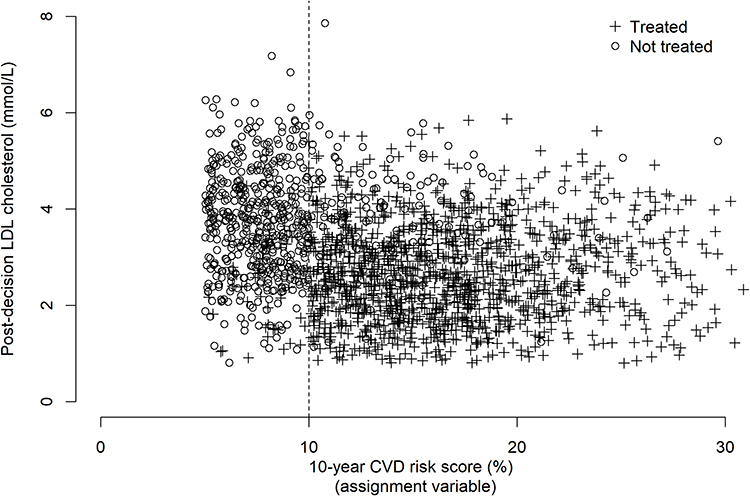Figure 9 Scatter plot showing post-decision LDL cholesterol (the outcome) against 10-year CVD risk score (the assignment variable) with icons to indicate treatment/non-treatment. A + symbol denotes an individual that receives statins, a ○ symbol denotes an individual that does not receive statins.

In Figure 9, we see that treatment tends to occur more often above the 10% threshold. However, as noted earlier, showing individual points can make this plot difficult to interpret. To investigate the discontinuity further, Figure 10 shows a plot of the empirical probability of treatment, calculated for subgroups of individuals against the 10-year CVD risk score.

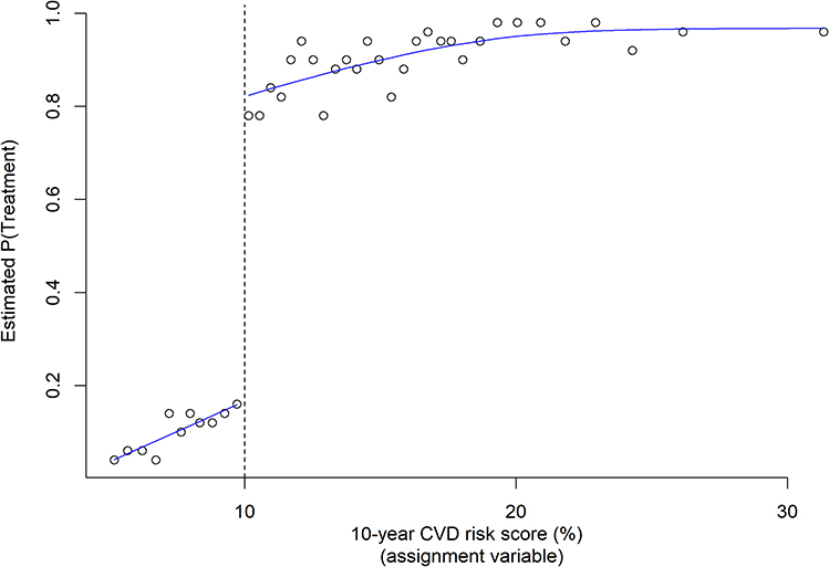Figure 10 Empirical estimates of the probability of being prescribed statins, by risk score group. Risk scores were grouped into bins containing equal numbers of individuals, and the proportion of individuals who receive statins calculated for each bin.

The discontinuity in the probability of treatment either side of the threshold is clear and, therefore, we will fit a fuzzy RDD to these data, to estimate the effect of statins on LDL cholesterol at the threshold. We now demonstrate the use of both the continuity-based and local randomisation RDDs, using this data example.

Continuity-Based Estimation

For the continuity-based approach, we choose the order of the models to be 2. In other words, we assume a quadratic relationship between the 10-year CVD risk score and LDL cholesterol level. This choice represents a slightly flexible model but not with too many higher order terms so as to overfit the data. The R output from fitting this model is shown in Figure 11.

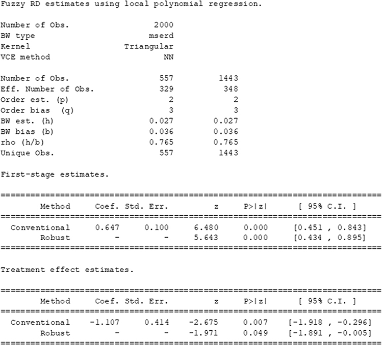Figure 11 R output from fitting a continuity-based RDD to the example dataset on statin prescription according to 10-year CVD risk score.

We see that the chosen bandwidth is 0.027, implying that individuals with 10-year CVD risk probabilities between 0.073 and 0.127 (ie 7.3% and 12.7%) have been included in the design. The estimate of the treatment effect of statins on LDL cholesterol at the threshold is −1.11, with robust 95% confidence interval (−1.89, -0.01). This suggests that in a region around the threshold, we might expect the LDL cholesterol level to be approximately −1.11 mmol/L lower for an individual who receives statins, compared to an individual who does not receive statins.

Local Randomisation Estimation

As noted previously, if we wish to use a local randomisation RDD (ie one that is similar to an RCT, but assuming quasi-randomisation) then we must first select a suitable window around the threshold, in which we expect individuals to be balanced with respect to potential confounding variables, that is, confounding variables for the statin – LDL cholesterol level relationship.

Typically, the window selection would be done by first discussing the data and RDD set-up with expert clinicians, who are likely to have knowledge and experience regarding similarities between individuals with similar 10-year CVD risk scores, around the threshold. In this example, we assume that, on discussion with clinical colleagues, a window of ±0.05 is chosen, around the threshold of 0.1 (ie a 10% 10-year CVD risk score).

Prior to fitting a local randomisation RDD, the sub-sample of individuals with 10-year risk scores ≥0.05 and ≤0.15 is taken. In our dataset, there are 557 individuals with risk scores ≥0.05 and <0.10 (ie within the window and below the threshold) and 628 individuals with risk scores ≥0.1 and <0.15 (ie within the window and above the threshold). Before fitting the local randomisation RDD, we compare these groups of individuals with respect to potential confounding variables: age (years), high density lipoprotein (HDL) cholesterol level, systolic and diastolic blood pressures, and current smoking status. Table 1 shows summary statistics for these variables, separately for groups of individuals with risk scores above and below the threshold, together with P-values for appropriate hypothesis test to compare the distribution of each variable between groups. In situations where sample sizes are large, an examination of standardised mean differences (for continuous variables) can be more informative than P-values from hypothesis tests because, in large sample sizes, small differences between groups that are not necessarily clinically relevant, may be statistically significant if a standard 5% significance level is assumed. Alternatively, appropriate controls for multiple hypothesis testing should be used, such as those discussed by Farcomeni.²³

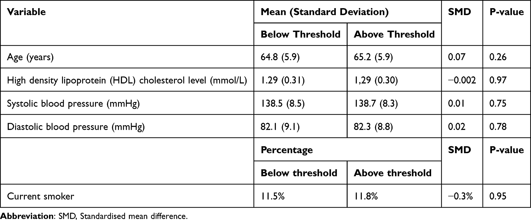Table 1 Summary Statistics for Possible Confounding Variables, Shown Separately for Groups of Individuals with 10-Year CVD Risk Scores Above and Below the 10% Threshold. The Standardised Mean Difference is Also Shown. P-values are Shown for Tests of the Null Hypothesis of No Difference in the Distribution of the Corresponding Variable, Between Groups

As noted previously, if we wish to use a local randomisation RDD (ie one that is similar to an RCT, but assuming quasi-randomisation) then we must first select a suitable window around the threshold, in which we expect individuals to be balanced with respect to potential confounding variables, that is, confounding variables for the statin – LDL cholesterol level relationship. Typically, the window selection would be done by first discussing the data and RDD set-up with expert clinicians, who are likely to have knowledge and experience regarding similarities between individuals with similar 10-year CVD risk scores, around the threshold. In this example, we assume that, on discussion with clinical colleagues, a window of ±0.05 is chosen, around the threshold of 0.1 (ie a 10% 10-year CVD risk score).

We compare groups of individuals above and below the threshold (within the RDD window) with respect to potential confounding variables: age (years), high density lipoprotein (HDL) cholesterol level, systolic and diastolic blood pressures, and current smoking status. Table 1 shows summary statistics for these variables, separately for groups of individuals with risk scores above and below the threshold, together with standardised mean differences and P-values for appropriate hypothesis tests to compare the distribution of each variable between groups.

R output from the fitted local randomization RDD is shown in Figure 12. The estimate of the treatment effect of statins on LDL cholesterol at the threshold is −1.080, with 95% confidence interval (−1.23, −0.93). This suggests that in a region around the threshold, we might expect the LDL cholesterol level to be approximately −1.08 mmol/L lower for an individual who receives statins, compared to an individual who does not receive statins. Notably, this is similar to the continuity-based estimate (−1.11) but the 95% confidence interval for the local randomisation estimate is narrower. This is probably because of the larger sample size (as the local randomisation window of ±0.05 is wider than the continuity-based bandwidth of ±0.027).

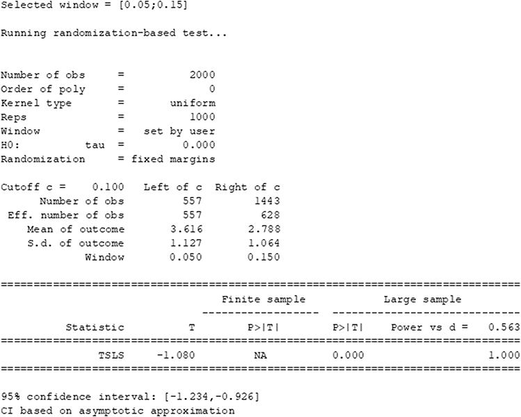Figure 12 R output from fitting a local randomisation RDD to the example dataset on statin prescription according to 10-year CVD risk score.

It is encouraging that the two approaches produce similar treatment effect estimates and, in this case, either RDD approach is likely justifiable. In some cases, the continuity-based approach could be more appropriate than the local randomization RDD, especially if it is suspected that there is a strong relationship between the assignment variable and outcome, either side of the threshold.

In practice, it may be that a local randomisation RDD is preferable – especially in scenarios where the RDD setup naturally mimics a RCT (eg where a prescription/intervention occurs based on a clearly defined rule) and there is clear similarity between groups either side of but close to the threshold, with respect to confounding variables. In situations where the “intervention” occurs more naturally rather than prescriptively (eg where the cut-off is age or location-based) a continuity-based RDD may be more appropriate. However, we note that, where assumptions are valid, either approach is feasible and it is essential to consider the decision rule, available data and question of interest – together with checks of key assumptions – prior to applying an RDD.

Discussion

This paper provides an overview of the regression discontinuity design and its use as a method for treatment/intervention effect estimation in epidemiological research. We outlined the general scenario in which an RDD is applicable – that where a treatment or intervention is assigned according to decision rule linked to a continuous assignment variable and considered the established continuity-based and local randomisation estimation approaches.

An RDD relies on specific assumptions that should be carefully considered and justified prior to modelling and estimation. In particular, the continuity-based approach relies on the choice of a kernel and polynomial form for the assignment variable-outcome relationship. In contrast, the local randomisation approach relies on the assumption of balanced groups with respect to potential confounding variables, in the assignment variable window around the threshold in which the RDD applies. In either case, an RDD is applicable only for scenarios in which the assumptions hold. As such, justification of these assumptions is a crucial part, and first step, when an RDD is applied to epidemiological data. Good practice involves extensive discussions amongst research teams (typically involving statisticians, epidemiologists, clinicians and/or other health care researchers) to ensure that groups above and below the treatment/intervention threshold are balanced with respect to potential confounding variables and that other RDD assumptions are valid. In addition, exploratory plots should be used to check that a discontinuity exists at the threshold, with respect to treatment/intervention assignment. If no such discontinuity exists, the RDD will not be appropriate. Even if a discontinuity with respect to treatment/intervention is apparent at a particular threshold, it should be checked that individuals were allocated to treatment/intervention according to a decision rule and that systematic manipulation of this rule, by individuals or clinicians, was not used to receive (or not receive) the treatment/intervention.

It is important to remember that the treatment/intervention effect estimate is valid only in a region around the threshold: the RDD does not estimate a global treatment/intervention effect. Although this may appear to be a drawback of the RDD, a randomised experiment is usually carried out under strict inclusion/exclusion criteria, often leading to restrictive treatment/intervention effect estimates in RCTs.

RDDs differ from other quasi-experimental approaches, such as difference-in-difference designs and instrumental variable (IV) methods. With difference-in-difference designs, a change over time with respect to an outcome is compared between “treated” and “untreated” groups, with differencing used to account for confounding. IV methods rely on a variable that is correlated with treatment assignment and used as an “instrument” for treatment. However, this method does not include a decision-based threshold or assumptions regarding the similarity of groups within a given region.

We have considered only RDDs with continuous (non-time-to-event) outcomes where the assignment variable is measured once. Extensions to the standard RDD include methods for binary and time-to-event outcomes,^11,12,24 cases in which multiple thresholds are used²⁵ and others where clustering occurs.²⁶ Large-scale electronic health care records together with many questions of interest related to treatment/intervention effects from decision rules provide substantial opportunities for further RDD developments in epidemiology. The RDD is a useful alternative or complement to RCTs and can apply to larger and more diverse groups than those that meet RCT eligibility criteria. This can allow a “real-world” estimate of a treatment/intervention effect, which is valuable in epidemiological research. We recommend that more empirical applications of the RDD be undertaken in health care and epidemiological research.

References

1. National Institute for Health and Care Excellence (NICE). Cardiovascular disease: risk assessment and reduction, including lipid modification. NG238; 2023. Available from: https://www.nice.org.uk/guidance/ng238.
2. Hippisley-Cox J, Coupland C, Brindle P. Development and validation of QRISK3 risk prediction algorithms to estimate future risk of cardiovascular disease: prospective cohort study. BMJ. 2017;357:j2099. doi:10.1136/bmj.j2099
3. National Institute for Health and Care Excellence (NICE). Adrenal insufficiency: identification and management. NG243; 2024. Available from: https://www.nice.org.uk/guidance/ng243.
4. National Institute for Health and Care Excellence (NICE). Type 2 diabetes: prevention in people at high risk. PH38; 2017. Available from: https://www.nice.org.uk/guidance/PH38.
5. Imbens GW, Lemieux T. Regression discontinuity designs: a guide to practice. J Econom. 2008;142(2):615–635. doi:10.1016/j.jeconom.2007.05.001
6. Lee DS, Lemieux T. Regression discontinuity designs in economics. J Econ Lit. 2010;48:281–355. doi:10.1257/jel.48.2.281
7. Dicks A, Lancee B. Double disadvantage in school? Children of immigrants and the relative age effect: a regression discontinuity design based on the month of birth. Euro Sociol Rev. 2018;34(3):319–333. doi:10.1093/esr/jcy014
8. Kirkland PA, Phillips JH. A regression discontinuity design for studying divided government. State Politics Policy Q. 2020;20(3):356–389. doi:10.1177/1532440019896981
9. Moscoe E, Bor J, Barnighausen T. Regression discontinuity designs are underutilized in medicine, epidemiology, and public health: a review of current and best practice. J Clin Epidemiol. 2016;68(2):132–143. doi:10.1016/j.jclinepi.2014.06.021
10. Boon MH, Craig P, Thomson H, Campbell M, Moore L. Regression discontinuity designs in health: a systematic review. Epidemiology. 2021;32:87–93. doi:10.1097/EDE.0000000000001274
11. Adeleke MO, O’Keeffe AG, Baio G. Approaches to risk ratio estimation in a regression discontinuity design: application to the prescription of statins for cholesterol reduction in UK primary care. Statis Methods Med Res. 2023;32(10):1994–2015. doi:10.1177/09622802231192958
12. Adeleke MO, Baio G, O’Keeffe AG. Regression discontinuity designs for time-to-event outcomes: an approach using accelerated failure time models. J R Stat Soc Ser A. 2022;185(3):1216–1246. doi:10.1111/rssa.12812
13. Imbens GW, Angrist JD. Identification and estimation of local average treatment effects. Econometrica. 1994;62(2):467–475. doi:10.2307/2951620
14. Hahn G, Todd P, Van der Klaauw W. Identification and estimation of treatment effects with a regression-discontinuity design. Econometrica. 2001;69(1):201–209. doi:10.1111/1468-0262.00183
15. Calonico S, Cattaneo MD, Titiunik R. Robust nonparametric confidence intervals for regression-discontinuity designs. Econometrica. 2014;82(6):2295–2326. doi:10.3982/ECTA11757
16. Calonico S, Cattaneo MD, Farrell MH. Optimal bandwidth choice for robust bias-corrected inference in regression discontinuity designs. Econometrics J. 2020;23:192–210. doi:10.1093/ectj/utz022
17. Calonico S, Cattaneo MD, Titiunik R. rdrobust: an R package for robust nonparametric inference in regression-discontinuity designs. R J. 2015;7(1):38–51. doi:10.32614/RJ-2015-004
18. Calonico S, Cattaneo MD, Titiunik R. Robust data-driven inference in the regression-discontinuity design. Stata J. 2014;14(4):909–946. doi:10.1177/1536867X1401400413
19. Cattaneo MD, Titiunik R, Vazquez-Bare G. rdlocrand: local randomization methods for RD designs. R package version 1.0; 2022. Available from: https://CRAN.R-project.org/package=rdlocrand.
20. Cattaneo MD, Titiunik R, Vazquez-Bare G. Inference in regression discontinuity designs under local randomization. Stata J. 2016;16(2):331–337. doi:10.1177/1536867X1601600205
21. Cattaneo MD, Titiunik R, Vazquez-Bare G. Power calculations for regression-discontinuity designs. Stata J. 2019;19(1):210–245. doi:10.1177/1536867X19830919
22. Geneletti S, O’Keeffe AG, Sharples LD, Richardson S, Baio G. Bayesian regression discontinuity designs: incorporating clinical knowledge in the causal analysis of primary care data. Stat Med. 2015;34(15):2334–2352. doi:10.1002/sim.6486
23. Farcomeni A. A review of modern multiple hypothesis testing, withparticular attention to the false discovery proportion. Statis Methods Med Res. 2008;17(4):347–388. doi:10.1177/0962280206079046
24. Geneletti S, Ricciardi F, O’Keeffe AG, Baio G. Bayesian modelling for binary outcomes in the regression discontinuity design. J R Stat Soc. 2019;182(3):983–1002. doi:10.1111/rssa.12440
25. Bertanha M. Regression discontinuity design with many thresholds. J Econom. 2020;218(1):216–241. doi:10.1016/j.jeconom.2019.09.010
26. Bai F, Kelcey B, Xie Y, Cox K. Design and analysis of clustered regression discontinuity designs for probing mediation effects. J Exp Educ. 2023;1–31. doi:10.1080/00220973.2023.2287445
© 2025 The Author(s). This work is published and licensed by Dove Medical Press Limited. The
full terms of this license are available at https://www.dovepress.com/terms
and incorporate the Creative Commons Attribution
- Non Commercial (unported, 4.0) License.
By accessing the work you hereby accept the Terms. Non-commercial uses of the work are permitted
without any further permission from Dove Medical Press Limited, provided the work is properly
attributed. For permission for commercial use of this work, please see paragraphs 4.2 and 5 of our Terms.