Optic disc segmentation for glaucoma screening system using fundus images

Introduction

Glaucoma is a chronic eye disease in which the optic nerve is gradually damaged. Glaucoma is the second leading cause of blindness after cataract, with ~60 million cases reported worldwide in 2010.¹ It is estimated that by 2020, about 80 million people will suffer from glaucoma.¹ If untreated, glaucoma causes irreversible damage to the optic nerve and can lead to blindness. Therefore, diagnosing glaucoma at early stages is extremely important for proper management and successful treatment and control of the disease.^2–4 In addition to the visual field test and intraocular pressure measurement, precise measurement of the disc and cup areas as well as the cup to disc ratios is important for accurate diagnosis of glaucoma and for diligent follow-up of progression of glaucoma. Currently, the cup to disc ratios are assessed manually by the professionals, and due to their different levels of expertise and experience, the results of such subjective assessments vary considerably.⁵

Numerous studies have been published on automated segmentation of the optic disc (OD). A good critical review of the literature on glaucoma image processing was given by Almazroa et al.⁶

The level set method for OD segmentation was used by Wong et al⁷ by applying a novel vibrational level set function proposed by Li et al⁸ on the red channel of the fundus image. The algorithm was tested on 104 images. Due to the influence of blood vessels, the level set was not accurate. Therefore, the red channel was not efficient to remove the blood vessels and the algorithm has to be tested on more images with different aspects. In another study by Yu et al,⁹ the OD was localized using template matching; then the blood vessels were removed by a morphologic filtering. Finally, a level set model¹⁰ that combines the region information and local edge vector to drive the deformable contour was applied to detect the disc boundaries. The algorithm was tested using 1,200 fundus images from MESSIDOR dataset,¹¹ where the average error in area overlap was 11.3% and the average absolute area error was 10.8%. Another study introduced the template matching model and the level set method by Wang et al.¹² The OD was localized using template matching, while the disc was segmented using the level set method. Furthermore, an energy function was developed to obtain better segmentation after removing the blood vessels by applying a closing morphologic operation. The algorithm was tested on 259 fundus images from three different sources based on seven performance measurements. The average overlap percentages were 88.17% (DRIVE dataset), 88.16% (DIARETDB1 dataset), and 89.06% (DIARETDB0 dataset).^13–15

Yin et al¹⁶ introduced an edge detection, circular Hough transform, to estimate the OD center and diameter and a statistical deformable model to adjust the disc boundary according to the image texture. The method was tested on 325 images. The average error in area overlap was 11.3% and the average absolute area error was 10.8%. Cheng et al¹⁷ also achieved good results by eliminating the peripapillary atrophy based on edge filtering, constraint elliptical Hough transform, and peripapillary atrophy detection. Due to the low contrast of the disc boundary, OD boundary was not detected in some images. Therefore, a preprocessing stage to select the best image component was necessary to improve the results. The algorithm was tested on 650 images and the overlap error was 10%.

Methodology

Dataset

Retinal images for glaucoma analysis (RIGA) dataset was collected to facilitate research on computer-aided diagnoses of glaucoma. The dataset has received an ethics clearance from the office of research ethics in University of Waterloo, Canada. The dataset consists of 750 color fundus images gained from three different sources: 1) 460 images were obtained from MESSIDOR dataset with two image sizes, 2,240×1,488 pixels and 1,440×960 pixels, and 2) 195 images were obtained from Bin Rushed Ophthalmic Center in Riyadh, Saudi Arabia. They were acquired in 2014 using a Canon CR2 non-mydriatic digital retinal camera. The dataset contains both normal and glaucomatous fundus images. The image size is 2,376×1,584 pixels. An additional 95 images obtained from Magrabi Eye Center in Riyadh, Saudi Arabia served as the third source. The images were collected between 2012 and 2014 using a Topcon TRC 50DX mydriatic retinal camera. The image size is 2,743×1,936 pixels. The images were marked manually by each of the six ophthalmologists. Each ophthalmologist marked the disc and cup boundaries manually using a precise pen for Microsoft Surface Pro 3 with 12 inches high-resolution screen (2,160×1,440 pixels). Six parameters were calculated for the manual marking, in order to be used to evaluate the algorithm, namely, disc area, disc centroid, cup area, cup centroid, vertical cup to disc ratio, and horizontal cup to disc ratio. This dataset was used for the subsequent image processing procedures. The dataset was split into two sets: 200 images for training and 550 images for testing.

OD localization

To facilitate the processing, a localizing technique was applied to separate the region of interest from the entire image. This procedure was introduced in Burman et al¹⁸ and Almazroa¹⁹ and involves using an Interval Type-II fuzzy entropy-based thresholding scheme along with Differential Evolution, which is a powerful meta-heuristic technique for faster convergence and less computational time complexity in order to determine the location of the OD. The multilevel image segmentation is a method to segment the image into various objects in order to find the brightest object of the image, which is located in the optic cup (OC) and, hence, is a part of the OD. The localization accuracy was 96.4% for all the 750 images.

OD algorithm

OD (optic nerve head) is the round area containing the cup where the ganglion cell axons leave the eye. The area between the cup boundaries and the disc boundaries is called neuroretinal rim area. Disc boundaries’ segmentation was concentrated on the borders between the disc and the retina.

In a healthy eye, the gradual intensity variation between the disc and retina is obvious. In some pathologic cases such as OD drusen, OD edema, peripapillary atrophy, and optic pits, the distinction might be less obvious, reducing the accuracy of disc boundary segmentation.

Figure 1 shows the algorithm details. Two hundred images from RIGA dataset were used in order to train the algorithm. After localizing the region of interest based on Burman et al,¹⁸ the blood vessels were extracted via a top-hat transform on the G-channel of the fundus image. Then, a fast digital image inpainting technique using a diffusion process²⁰ was applied on the extracted blood vessels. As the diffusion process is iterated, the inpainting progresses from the area boundary into the area itself. The user can specify the number of iterations, and therefore, the algorithm works perfectly to inpaint a small area of the image. Since the area is small, the inpainting procedure can be approximated by an isotropic diffusion process which spreads the information from the area boundaries into the area itself in the gray level image by repeatedly convolving the region to be inpainted with a diffusion kernel. Convolving an image with a Gaussian kernel (ie, computing weighted averages of pixels’ neighborhoods) is equivalent to isotropic diffusion. The algorithm uses a weighted average kernel that only considers contributions from the neighboring pixels. Increasing the inpainted area reduces the quality as well as the iteration numbers, making the process slower as shown later in the “Results of Magrabi dataset” section. The algorithm worked well with good-quality fundus images; however, it did not work properly with low-quality fundus images. With low-quality images, the blood vessels occupying big areas of the images made the process lengthy due to the greater number of iterations that needed to be applied in order to achieve good inpainting.

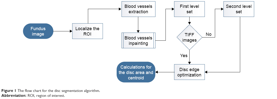Figure 1 The flow chart for the disc segmentation algorithm. Abbreviation: ROI, region of interest.

The disc segmentation algorithm used for RIGA dataset had two paths, one for TIFF images (MESSIDOR and Magrabi datasets) the second is for JPG images (Bin Rushed dataset). As illustrated in Figure 2, the algorithm was applied to TIFF images which have better contrast. Figure 2A represents the localized images. Figure 2B shows the inpainted image in red channel, where the contrast between the disc and the retina makes them easily distinguishable from each other and the inpainted algorithm had been set for 500 iterations. Therefore, the segmentation process represented by the active contour model implemented by the level set⁸ was easy and more accurate, as shown in Figure 2C. With trial and error, the level set was set to 70 iterations in order to have the best disc boundary detection. However, the disc edge was influenced by the blood vessels, as shown in Figure 2C. Therefore, a disc edge optimization algorithm was developed in order to optimize the disc edges and improve the accuracy (as shown in Figure 2D) by converting the segmented disc to binary image and calculating the central point of circle disc edge and making it the origin of the coordinate system. From the central point, the angles and the corresponding radius of each disc edge point to origin were calculated in order to compute the differences among radiuses to the angles. With the prior knowledge that every part of disc edge should be a smooth curve, the big difference between the radius of neighboring edge points was computed in order to detect where the disc edge was influenced by the blood vessels, and then, the edge was optimized by correcting the radius.

Figure 2 The disc segmentation procedure for TIFF images (MESSIDOR and Magrabi). (A) Localized image; (B) inpainted image; (C) segmented disc boundaries; (D) optimized disc.

JPG images went through more processing due to their low contrast quality. In Figure 3, the second column of the first row represents the inpainted image in red channel. Still some blood vessels appeared after inpainting; however, they did not affect the segmentation process. The third column represents the first level set applied on the inpainted image, and it is clear that the first level set went outside the actual boundary. Therefore, the first level set was considered as the first contour for OD in order to eliminate the big contrast variation that reduces the accuracy. After localizing the OD again and obtaining the rough disc boundaries after the level set, the new localized image was split into left and right disc by a central point as shown in the fourth column. Finally, the second level set was applied on each of the two parts. The final results are shown in the fifth column. An edge optimization algorithm was needed to improve the contour in this image. In the second row, the first level set shows the worst case due to the big variation in the retina, specifically in the top right area of the image.

Figure 3 The disc segmentation procedure for JPG images (Bin Rushed): (A) localized fundus image, (B) inpainted image, (C) first level set, (D) the localized image based on the first level set (is split from the middle), (E) second level set, (F) optimized disc contour.

Sometimes there were blank areas in the concatenated disc edge from double level set, which could deteriorate the result. Therefore, blank elimination was developed to restore the edge by automatically detecting blank areas through analysis of the radius to angle and inpainting the edge binary image by adding some edge points to the blank according to the radius and angles of the two breakpoints in the blank.

Results

The simulation was performed in Matlab 2014b environment in a workstation with Intel Core i-7 2.50 GHz processor. As seen in Figure 4, the disc segmentation algorithm went through the same steps that were used by the six ophthalmologists to evaluate the agreement on the images (presented in Almazroa¹⁹). First of all, the images of the six ophthalmologists were filtered based on the mean SD for the disc area and centroid. 1) The disc areas for all the manual marking images (six manual marking images for every single image of the dataset) were calculated; then, the SDs among the six manual marking areas for every image were computed. Finally, the mean SD for all the calculated SDs was chosen to be the judge for every image, that is, every image had six manual markings. Therefore, the SD for this image was calculated and compared with the mean SD. If the SD > mean SD, this means an outlier (manual marking > than others) needs to be removed in order to make the SD equal to or smaller than the mean SD. The mean SD will be variable between the three images dataset due to the variability of the image sizes since the images sizes are different from dataset to another, these are reflected on the discs’ sizes (disc areas). Therefore, the mean SDs are not constant to all three datasets (Figure 4) (Bin Rushed ≤1,650, Magrabi ≤6,400 and MESSIDOR ≤1,500 pixels). If there were three or more manual markings, the images were removed; this means there was a big variation among the ophthalmologists (variation on disc areas). As a result, this specific image was not eligible to train and test any algorithm. 2) These procedures were conducted on the centroid calculations.

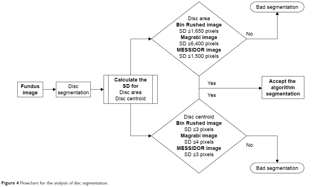Figure 4 Flowchart for the analysis of disc segmentation.

Secondly, after filtering the manual marking and only keeping the images with SD < mean SD, the algorithm area and centroid were considered to be a seventh ophthalmologist, thus, if the segmented disc area or centroid makes the SD with the six ophthalmologists disc manual marking ≤ the mean SD, that will become a good segmentation; otherwise, it is a bad segmentation result. This procedure was conducted for all the images. Then, the number of segmented images giving good results were considered for accuracy, comparing it with the filtered images.

The images with OD area and centroid agreed upon by at least four ophthalmologists were selected and used to evaluate the new algorithm. For every segmented image, the area and centroid were calculated in order to test their accuracy by comparing the newly computed SDs with those computed by the ophthalmologists as well as the algorithm, and then it was decided whether the segmentation was acceptable or not.

The results of automatic segmentation and manual markings by the six ophthalmologists are compared in Figure 5. The first column represents the manual marking by the first ophthalmologist, the second column by the second ophthalmologist, and so on. The seventh column represents the result of the automatic segmentation by the algorithm. The first image is represented in the first row, the second image in the second row, and so on. As noted in Almazroa,¹⁹ the mean SD was 1,500 pixels for the disc area and 3 pixels for centroid for MESSIDOR dataset. The manual markings by ophthalmologists number one and six were eliminated (since they were outliers in terms of area) from the first image (MESSIDOR image). Using the remaining images (those marked by the other four ophthalmologists) for analysis of the area, the algorithm gave 1,550 pixels as SD and 3 pixels as SD of the centroid. For the second image (MESSIDOR image), the manual markings by the first ophthalmologist were eliminated, since they were outliers in terms of centroid. The algorithm SD was 1,600 pixels for area and 2.5 pixels for centroid. In the third image (Bin Rushed image), the markings by the first ophthalmologist were removed, since the measurements of the centroid done by this ophthalmologist increased the SD for all manual markings to >3 pixels. The SD calculated by the algorithm was 2.5 pixels for centroid and 1,100 pixels for area. In the last image (Bin Rushed image), the manual markings by ophthalmologists number one and three were considered as outliers in terms of area. The algorithm SD was 4 pixels for centroid and 1,800 pixels for area, which were acceptable. In Figure 6, the first image shows a huge variation in the markings of the six ophthalmologists. Markings of ophthalmologists number one and two were considered as outliers in terms of centroid. Markings of ophthalmologist number three were considered as outliers in both area and centroid. The algorithm produced very poor results for both area and centroid. The right side of the disc boundaries was not clear due to some abnormalities. We conclude that this image should not be considered for evaluating the algorithm, since the markings done by at least three ophthalmologists were eliminated due to outliers. In the second image, the Y axis of the centroid as marked by ophthalmologist number six was an outlier. The algorithm gave poor results for both area and centroid due to the fact that the right and lower sides of the disc boundaries had almost the same intensity. In the third image, there were no outliers in the markings by any of the six ophthalmologists. The algorithm gave good results in terms of area and centroid. In the last image, the markings by ophthalmologists number two, three, and four were outliers in terms of area, while the markings by ophthalmologists number five and six were outliers in terms of centroid. Therefore, this image was not considered for evaluating the algorithm. This indicates that in this procedure, the best agreed upon image was precisely selected to be used for evaluating the algorithm.

Figure 5 Examples of good disc segmentation results for both TIFF (MESSIDOR and Magrabi) and JPG (Bin Rushed) images comparing with those of six ophthalmologists.

Figure 6 Examples of bad disc segmentation results for both TIFF (MESSIDOR and Magrabi) and JPG (Bin Rushed) images comparing with those of six ophthalmologists.

Results of Bin Rushed dataset

Table 1 shows the results for Bin Rushed dataset. The algorithm was tested on 195 images. Ten images could not be localized. For area, an additional seven images were eliminated, since their area markings by three ophthalmologists were outliers. Therefore, in total, 178 images were tested for area and the accuracy was 155 images or 88.2%. On the other hand, 15 images were eliminated from the analysis of centroid. Therefore, in total, 170 images were tested for centroid and the accuracy was 149 images or 87.6%. Thirty-four images were removed based on the analysis of both area and centroid. Many images were good in area, but had problems in centroid and vice versa. In total, 151 images were tested for both area and centroid and the accuracy was 130 images or 86%.

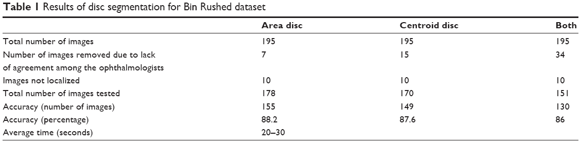Table 1 Results of disc segmentation for Bin Rushed dataset

The accuracy of markings by each ophthalmologist is presented in Table 2. If for an image there were at least three outliers in terms of disc area or centroid in the markings by five ophthalmologists, then the image was eliminated from measuring the accuracy of markings by the sixth ophthalmologist. The algorithm’s accuracy, however, was evaluated based on the markings by each of the six ophthalmologists. Based on the 156 images tested, markings by ophthalmologist number four with 92.9% accuracy were the most accurate. The algorithm results were the second best. The algorithm was tested using 151 images and the accuracy was 86%. Markings by ophthalmologists number six and five were next in terms of accuracy. Ophthalmologists number six and five tested 163 and 162 images and their accuracies were 85.2% and 84.5%, respectively. The average computation time was between 20 and 30 seconds for this dataset due to the number of iterations set for the level set as well as the inpainting. Between 19 and 34 images were eliminated due to lack of agreement, which represent 9% and 17% of the total number of images in the dataset, respectively.

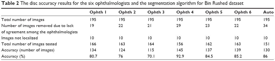Table 2 The disc accuracy results for the six ophthalmologists and the segmentation algorithm for Bin Rushed dataset

Results of Magrabi dataset

Table 3 shows the results of the second image source for RIGA dataset. Ninety-five images were tested, from which six images were not localized. In terms of area, eight images were eliminated because of the huge variation among markings by the six ophthalmologists. Therefore, in total, 81 images were tested. Seventy-three images (90.1%) were segmented successfully. On the other hand, 10 images were removed from the analysis of centroid. Therefore, in total, 79 images were tested for centroid and the accuracy was 89.8%. When testing for both the area and centroid, 21 images were eliminated. Therefore, in total, 68 images were tested for both the area and centroid, from which 61 images were correctly segmented (89.7% accuracy). The images that were taken with no mydriatics seemed less accurate than those with mydriasis images. However, the algorithm took 70–120 seconds to run Magrabi dataset, which is much longer than the time required to run Bin Rushed dataset. This was due to the fact that the images in Magrabi dataset were larger than the images in the other two datasets.

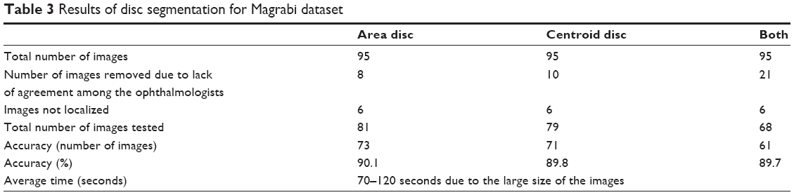Table 3 Results of disc segmentation for Magrabi dataset

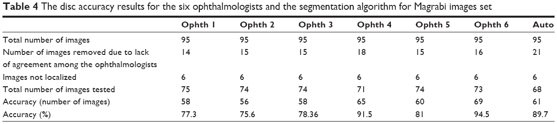
The markings by ophthalmologist number four for this dataset were highly accurate (Table 4). Sixteen images were removed due to the variations among markings by the ophthalmologists. Therefore, in total, 73 images were tested and the accuracy was 94.5%. Ophthalmologist number two had the second best markings. Here, 18 images were eliminated, hence 71 were tested and the accuracy was 91.5%. The algorithm came in the third best place, where the total number of images tested was 68 (less than the previous two) and the accuracy was 89.7%, and 14–21 images, that is, 14%–22% of the total number of images in the dataset, were eliminated from the test.

Table 4 The disc accuracy results for the six ophthalmologists and the segmentation algorithm for Magrabi images set

Results of MESSIDOR dataset

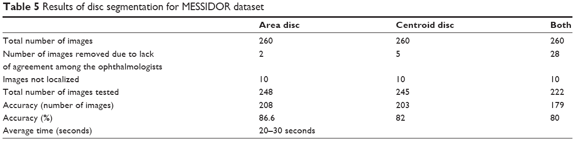
The last dataset used to evaluate the algorithm was MESSIDOR dataset with 260 images (Table 5). From this dataset, 10 images were not localized. Only two images were removed from analysis of area, hence 248 images were tested for area. Forty images were unsuccessfully segmented; therefore, the accuracy was 86.6%. Five images were eliminated from centroid evaluation. Therefore, in total, 245 images were tested for centroid. Forty-two images failed in this test, that is, the accuracy was 82%. When testing for both area and centroid, 28 images were removed; therefore, 222 images were tested and the accuracy was 80%. It took 20–30 seconds to run MESSIDOR dataset, which is the same as the time required to run Bin Rushed dataset. This is due to the fact that the images in these two datasets were similar in size.

Table 5 Results of disc segmentation for MESSIDOR dataset

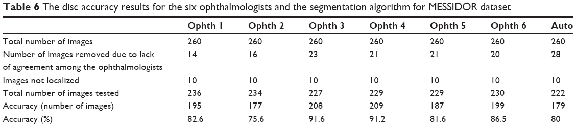
Based on the data presented in Table 6, ophthalmologists number three and four showed the best performance in manual marking, using a total of 227 and 229 images and showing 91.6% and 91.2% accuracy, respectively. The algorithm accuracy in this dataset was the second last and was close to that of ophthalmologists number five and one. In total, 14–28 images (5%–10.7% of images) were eliminated. Magrabi dataset had the greatest percentage of eliminated images, followed by Bin Rushed dataset, and finally MESSIDOR dataset. The variations in the markings of the three image sets obviously influenced the agreement and this is represented in the variation in the mean SD.

Table 6 The disc accuracy results for the six ophthalmologists and the segmentation algorithm for MESSIDOR dataset

Consolidated results

This section presents a comprehensive evaluation of markings done either automatically by the algorithm or manually by the six ophthalmologists. In total, 550 images were used from three image sources of RIGA dataset (Table 7), from which 26 images were not localized. Seventeen images were eliminated from area evaluation. The total number of images tested for area was 507, and the number of successfully segmented images was 436 (85.9%). Thirty images were eliminated from evaluation of centroid accuracy. Therefore, a total of 494 images were tested for centroid and 423 images (85.6%) were successfully segmented. Eighty-three images were eliminated from the analyses of both area and centroid. In total, 441 images were tested for both area and centroid, from which 71 images failed in segmentation, giving the final accuracy of 83.9% for the disc segmentation algorithm for RIGA dataset.

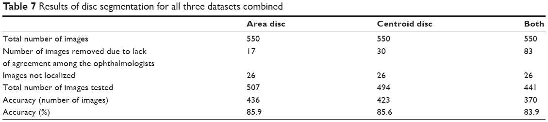Table 7 Results of disc segmentation for all three datasets combined

Table 8 compares the accuracy of disc segmentation in terms of disc area and centroid. Ophthalmologist number four used 472 images for disc manual marking and obtained the best result (88.7% accuracy). Ophthalmologist number six was the second best in disc manual marking, testing 466 images with 87.3% accuracy. The algorithm was the third best in disc boundaries marking. The algorithm tested 441 images with 83.9% accuracy. The lowest accuracy was 75.7%, based on testing 471 images (ophthalmologist number two). In conclusion, the accuracy of marking disc boundaries was high for both manual marking and automatic segmentation due to the clarity of the disc intensity. The greatest challenges were the abnormalities occurring on the two sides of the disc boundaries.

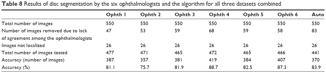Table 8 Results of disc segmentation by the six ophthalmologists and the algorithm for all three datasets combined

Figure 7 shows the variation in the performance on the three datasets. Ophthalmologists number one, two, four, and five showed similar performance, regardless of the dataset used. Ophthalmologist number three showed different performance; he/she performed best for MESSIDOR dataset and worst for Bin Rushed dataset. Ophthalmologist number six showed a performance similar to that of the algorithm in terms of stability. Still, the lowest accuracy was around 70%, which was assumed to be high. Ophthalmologist number four showed a precise, stable, and high performance for detecting the disc boundaries, regardless of the dataset.

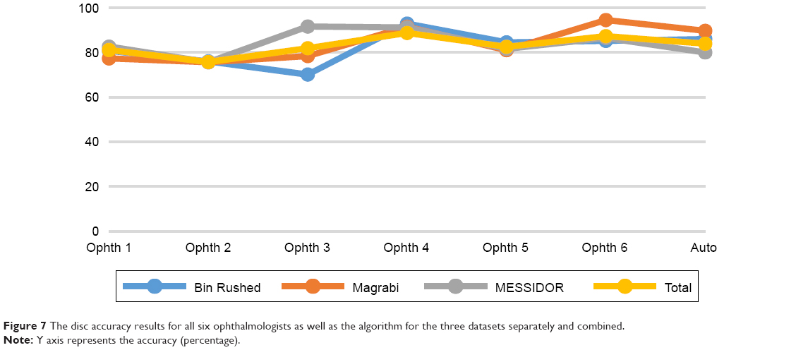Figure 7 The disc accuracy results for all six ophthalmologists as well as the algorithm for the three datasets separately and combined. Note: Y axis represents the accuracy (percentage).

Agreement for the disc

Table 9 shows the number of images agreed in the disc area and centroid among the six ophthalmologists as well as the disc segmentation algorithm. The accuracy calculations reflect how every ophthalmologist agreed with the others and who had the best performance. All the ophthalmologists had the best agreement with ophthalmologist number four, and then ophthalmologist number six. The least agreement was seen for the work of ophthalmologist number two. Ophthalmologist number three was the second last. The best agreement for the algorithm was with markings of ophthalmologist number four in 349 images (63.4%), while the lowest agreement was with markings of ophthalmologist number two in 316 images (57.4%). On the other hand, the best overall agreement was between the markings by ophthalmologists number four and six in 410 images (74.5%) and the lowest agreement was between the markings by ophthalmologists number two and three in 312 images (56.7%).

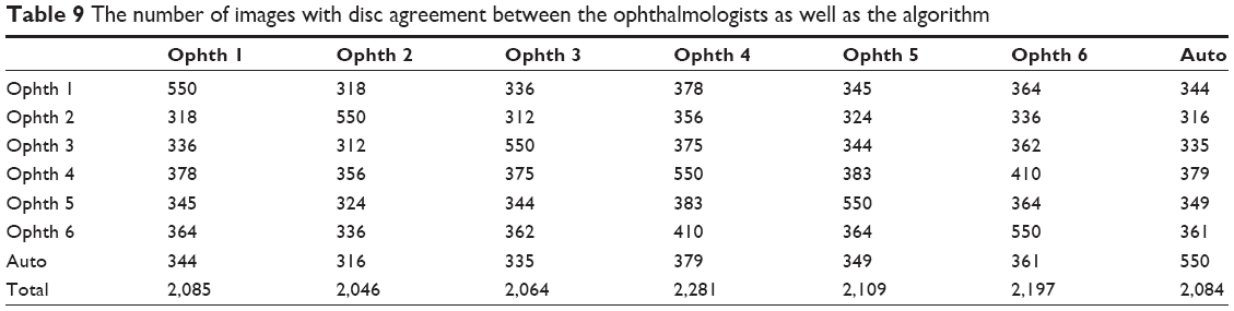Table 9 The number of images with disc agreement between the ophthalmologists as well as the algorithm

As the “Total” values in Table 9 indicate, markings by ophthalmologist number four were the best, followed by markings by ophthalmologist number six, ophthalmologist number five, the algorithm and ophthalmologist number one, ophthalmologist number three, and finally ophthalmologist number two. The accuracy of performance was the same for ophthalmologists number four, six, and two, followed by the algorithm, ophthalmologist number five, three, and finally ophthalmologist number one. As a result, having markings in a high number of images in agreement with the others does not mean good accuracy in disc detection. Figure 8 shows how the agreements are in groups.

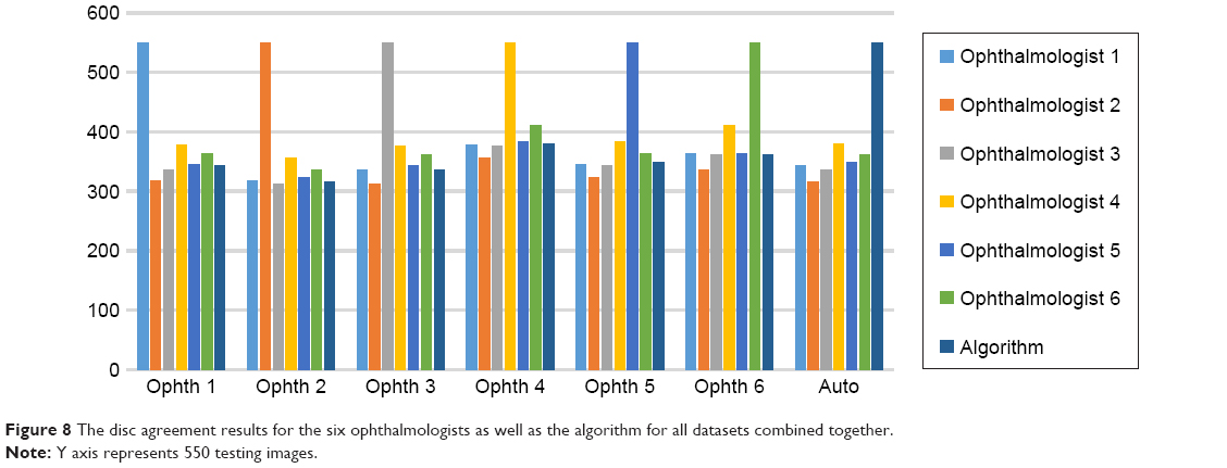Figure 8 The disc agreement results for the six ophthalmologists as well as the algorithm for all datasets combined together. Note: Y axis represents 550 testing images.

Figure 9 demonstrates how the ophthalmologists’ performance was regarding the agreement in the number of images. Clearly, ophthalmologist number four had the best agreement with the others due to the high accuracy in detecting the disc boundaries. He had 2,281 images, which was in agreement with all other five ophthalmologists in addition to the algorithm. On the other hand, ophthalmologist number two had the lowest agreement – only in 2,046 images. However, the difference between the highest and lowest agreement was only in 235 images, proving that all six ophthalmologists as well as the algorithm detected the disc boundaries similarly.

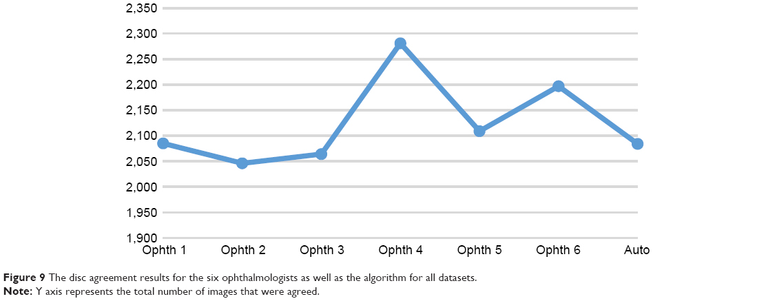Figure 9 The disc agreement results for the six ophthalmologists as well as the algorithm for all datasets. Note: Y axis represents the total number of images that were agreed.

Conclusion

A new OD segmentation algorithm for retinal image screening has been developed based on a unique dataset called RIGA. The opinions of multiple (six) ophthalmologists were considered to eliminate the errors that might occur during manual marking of disc and cup boundaries and increase the reliability of evaluation of the new algorithm. The OD area and centroid parameters were chosen to evaluate the new system in this paper. Most of the previous studies measured the overlapping between the segmented image and the manually marked image and then calculated the overlapping error. Therefore, the accuracy was based on how much was the overlap between the two images. The accuracy of the present algorithm has been computed based on the number of segmented images, keeping the SD of the tested images less than or equal to the mean SD of the six manual markings. This has an advantage over previous studies in which the manual marking was performed by only one person and the average of the overlapping accuracy was calculated.

The number of iterations for the level set as well as the inpainting process significantly affected the computational time. The computational time was 20–30 seconds for the small-size images of Bin Rushed and MESSIDOR datasets. On the other hand, the computational time for the large images of Magrabi dataset was 70–120 seconds, since it took longer to level set and inpaint the large images. The new automatic eye disease diagnosis system has to be robust, fast, and highly accurate, in order to support high workloads and near-real-time operation. The algorithm developed in this paper was designed to fulfill the aforementioned requirements. The robustness and efficiency of the proposed algorithm make it a suitable tool for automatic independent screening for signs of glaucomatous optic neuropathy in humans.²¹

Future work

Future work should consider disc abnormalities such as papillary atrophy, tilted discs, and disc drusen. More functions can be added to segment the pathologic disc boundaries better. The computational time can be reduced by developing an inpainting technique that requires less iterations.

Acknowledgments

The abstract of this paper was presented at the Medical Imaging 2017: Imaging Informatics for Healthcare, Research, and Applications conference as a conference talk with interim findings and was published in SPIE, Volume Number: 10138.

Disclosure

The authors report no conflicts of interest in this work.

---

References

1.		Quigley HA, Broman AT. The number of people with glaucoma worldwide in 2010 and 2020. Br J Ophthalmol. 2006;90(3):262–267.
2.		Costagliola C, Dell’Omo R, Romano MR, Rinaldi M, Zeppa L, Parmeggiani F. Pharmacotherapy of intraocular pressure: part I. Parasympathomimetic, sympathomimetic and sympatholytics. Expert Opin Pharmacother. 2009;10(16):2663–2677.
3.		Costagliola C, Dell’Omo R, Romano MR, Rinaldi M, Zeppa L, Parmeggiani F. Pharmacotherapy of intraocular pressure-part II. Carbonic anhydrase inhibitors, prostaglandin analogues and prostamides. Expert Opin Pharmacother. 2009;10(17):2859–2870.
4.		European Glaucoma Society. Terminology and Guidelines for Glaucoma. 4th ed. Savona: Italy: PubliComm; 2014:63.
5.		Inoue N, Yanashima K, Magatani K, Kurihara T. Development of a simple diagnostic method for the glaucoma using ocular Fundus pictures. Conf Proc IEEE Eng Med Biol Soc. 2005;4:3355–3358.
6.		Almazroa A, Burman R, Raahemifar K, Lakshminarayanan V. Optic disc and optic cup segmentation methodologies for glaucoma image detection: a survey. J Ophthalmol. 2015;2015:180972.
7.		Wong DK, Liu J, Lim JH, et al. Level-set based automatic cup-to-disc ratio determination using retinal fundus images in ARGALI. Conf Proc IEEE Eng Med Biol Soc. 2008;2008:2266–2269.
8.		Li C, Xu C, Gui C, Fox MD. Level set evolution without re-initialization: a new variational formulation. In Proceedings of the IEEE Computer Society Conference on Computer Vision and Pattern Recognition. San Diego, CA, USA; 2005:430–436. Available from: http://ieeexplore.ieee.org/xpls/abs_all.jsp?arnumber=1467299. Accessed August 28, 2017.
9.		Yu H, Barriga ES, Agurto C, et al. Fast localization and segmentation of optic disk in retinal images using directional matched filtering and level sets. IEEE Trans Inf Technol Biomed. 2012;16(4):644–657.
10.		Zhang Y, Matuszewski BJ, Shark LK, Moore C. Medical image segmentation using new hybrid level-set method. In Proc of the 5th International Conference of the BioMed. Visualization: Information Visualization in Medical and Biomedical Informatics; 2008:71–76. Available from: http://ieeexplore.ieee.org/xpls/abs_all.jsp?arnumber=4618616. Accessed August 28, 2017.
11.		MESSIDOR: Methods for Evaluating Segmentation and Indexing technique Dedicated to Retinal Ophthalmology. Image Analysis and Stereology. 2014:33(3):231–234.
12.		Wang C, Kaba D, Li Y. Level set segmentation of optic discs from retinal images. J Med Bioeng. 2015;4(3):213–220.
13.		Niemeijer M, Staal J, Ginneken B, Loog M, Abramoff M. DRIVE: digital retinal images for vessel extraction; 2004. Available from: http://www.isi.uu.nl/Research/Databases/DRIVE/. Accessed August 28, 2017.
14.		Kauppi T, Kalesnykiene V, Kamarainen J, et al. “DIARETDB0: Evaluation database and methodology for diabetic retinopathy algorithms”, Machine Vision and Pattern Recognition Research Group, Lappeenranta University of Technology: Finland; 2006. Available from: http://www2.it.lut.fi/project/imageret/diaretdb0/#COPY. Accessed August 28, 2017.
15.		Kauppi T, Kalesnykiene V, Kamarainen J, et al. “The DIARETDB1 diabetic retinopathy database and evaluation protocol”. BMVC. 2007: 1–10. Available from: http://www.it.lut.fi/project/imageret/diaretdb1/
16.		Yin F, Liu J, Ong SH, et al. Model-based optic nerve head segmentation on retinal fundus images. Conf Proc IEEE Eng Med Biol Soc. 2011;2011:2626–2629.
17.		Cheng J, Liu J, Wong DW, et al. Automatic optic disc segmentation with peripapillary atrophy elimination. Conf Proc IEEE Eng Med Biol Soc. 2011;2011:6224–6227.
18.		Burman R, Almazroa A, Raahemifar K, Lakshminarayanan V. Automated detection of optic disc in glaucoma. Adv Opt Sci Eng. Springer India. 2015;41:327–334.
19.		Almazroa A, Alodhayb S, Osman E, et al. Agreement among ophthalmologists in marking the optic disc and optic cup in fundus images. Int Ophthalmol. 2017;37(3):701–717.
20.		Oliveira MM, Bowen B, McKenna R, Chang YS. Fast digital image inpainting. In Proc of the international conference on Visualization, Imaging and Image Processing. 2001:106–107. Available from: http://www.inf.ufrgs.br/~oliveira/pubs_files/inpainting.pdf. Accessed August 28, 2017.
21.		Almazroa A, Alodhayb S, Raahemifar K, Lakshminarayanan V. An automatic image processing system for glaucoma screening. International Journal of Biomedical Imaging. 2017; ID 4826385.