Onset of mortality increase with age and age trajectories of mortality from all diseases in the four Nordic countries

Introduction

Aging is sometimes considered to be a continuous accumulation of damage and deterioration at the level of cells, tissues, organs, or organisms, which ultimately leads to death. The process is empirically responsible for the exponential relationship between mortality and age.^1–9 The answer to the question “At what age does aging begin?” is tightly related to the question “Where is the onset of mortality increase with age?” The onset of the exponential relationship between mortality and age has been studied.^10–12 The exponential increase of all-cause mortality with age empirically has started after the age of 35 years in developed countries during the last two centuries.^1,13–18 There are two possible explanations for exponential dependence not being observed before the age of 35 years: 1) the mechanism is switched on after the age of 35 years and 2) the exponential rise exists earlier, and is “overlapped” by nonbiological causes. The second possibility is demonstrated here, and age trajectories of all-disease mortality are modeled.

It is well known that age affects mortality from all diseases differently than it affects mortality from nonbiological causes.^1,13–15,19 Nonbiological causes (or external causes) are mostly accidents with specific relation to age. A typical step of total mortality is situated between 10 and 20 years of age (Figures 1–4). It is caused by nonbiological causes and disappears in the age trajectory of all-disease mortality. Nonbiological causes affect total mortality as the set of causes with a fractionally age-independent mortality rate.^13,15,19 These nonbiological causes are important to total mortality within the age range of 5–30 years, and they lose significance over the age of 40 years.^13,14,18 Typical age trajectories of mortality from all nonbiological causes for Norway in 1996 are shown as an example in Figure 1 in the log–log scale and concurrently in the semilogarithmic scale in Figure 2.

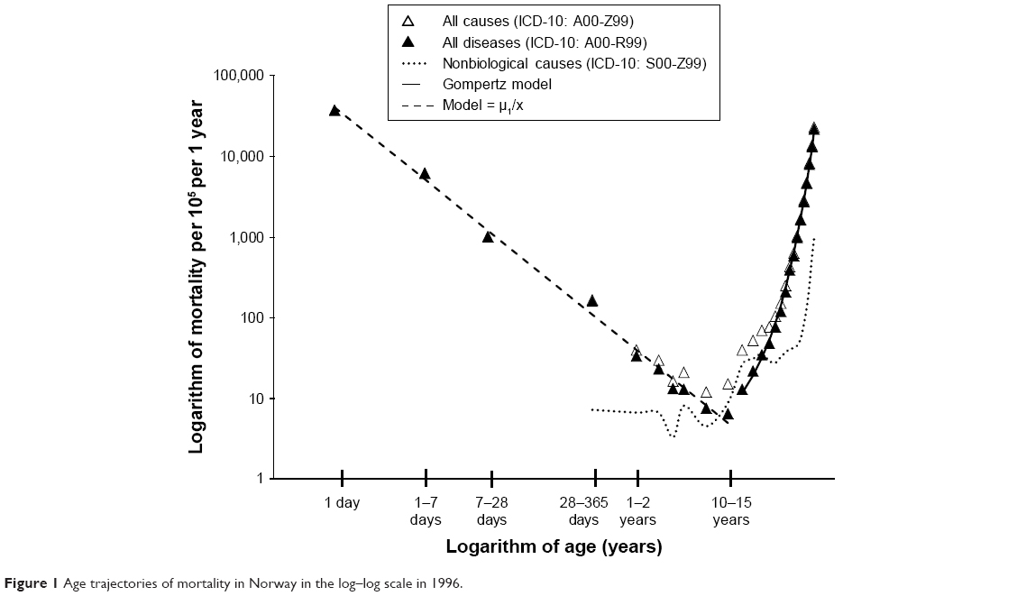Figure 1 Age trajectories of mortality in Norway in the log–log scale in 1996.

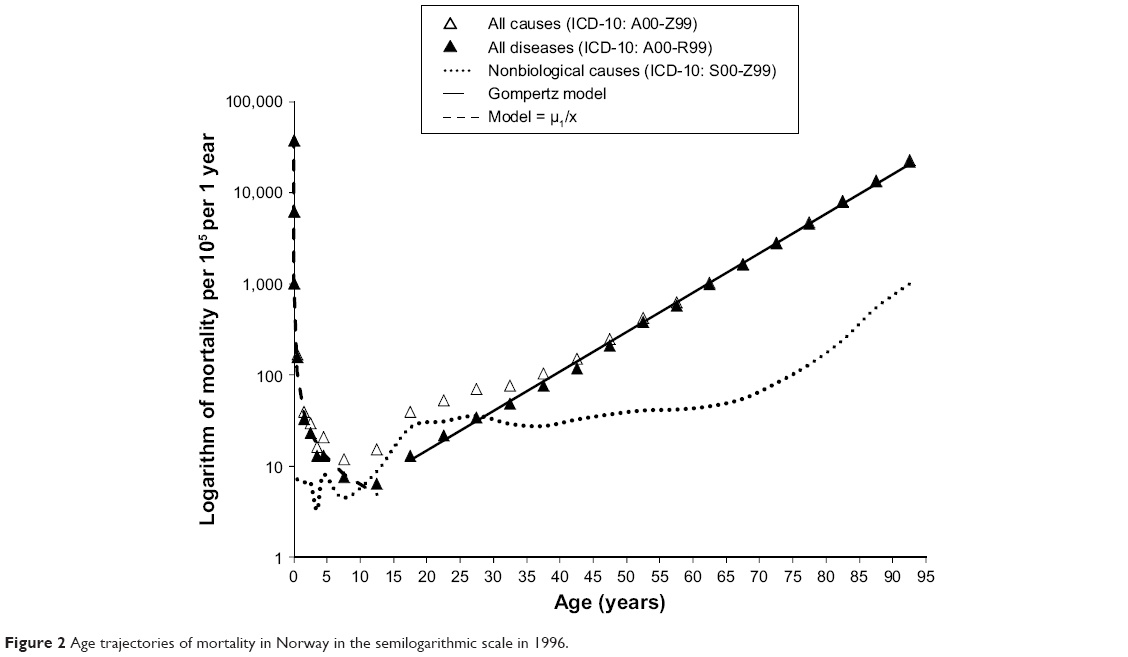Figure 2 Age trajectories of mortality in Norway in the semilogarithmic scale in 1996.

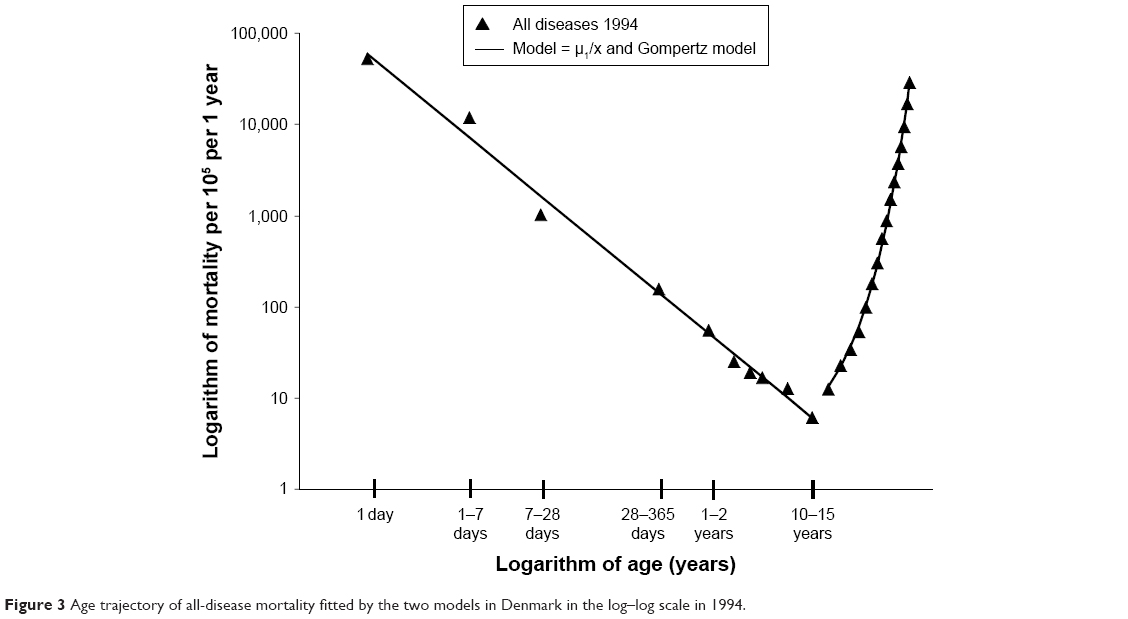Figure 3 Age trajectory of all-disease mortality fitted by the two models in Denmark in the log–log scale in 1994.

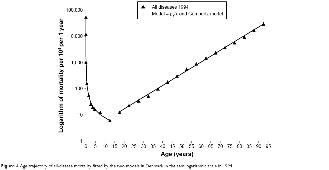Figure 4 Age trajectory of all-disease mortality fitted by the two models in Denmark in the semilogarithmic scale in 1994.

The impact of nonbiological causes could be demonstrated also by their fractions of total deaths. For example, they are between 0.51 and 0.73 in the specific age interval (5–30 years) in Nordic countries during the period 1994–2011. Total mortality rates in the Nordic countries within 5–30 years are very low, and the region represents extreme positive mortality. Age trajectories of mortality from all diseases in Denmark, Finland, Norway, and Sweden are analyzed here in all calendar years when the International Classification of Diseases (ICD)-10 classification of causes was used. The exclusion of nonbiological causes could be realized practically if information about detailed causes of death were known. Such information is available in the mortality database of the World Health Organization (WHO).²⁰ The ICD-10²¹ can identify nonbiological causes. The set of calendar years for every population is determined by the actual application of ICD-10 in a specific country.

Materials and methods

The number of deaths in the four countries for detailed causes of death in specific age categories was extracted from the file “Mortality, ICD-10”, available in the mortality database of the WHO.²⁰ The ICD-10 classification of causes of death is used in the database.²¹ The database usually uses the following 26 age intervals: 0–24 hours, 1–7, 7–28, and 28–365 days, and 1–2, 2–3, 3–4, 4–5, 5–10, 10–15… 90–95 years. The first age interval could be 0–1 year and the second interval 1–5 years in a specific country in a specific calendar year. If these two age categories are used in the database, then the construction of the age trajectory is not possible for ages up to 5 years, and such calendar years are excluded in a specific country. The result sets of calendar years used in every country are in the first column of Table 1. The resulting age trajectories of mortality from all diseases are constructed for the calendar years using the ICD-10 classification of four age categories in the first year and four age categories in the range of 1–5 years. For example, it represents nine age categories up to the age of 10 years. The database also contains the number of living people and the number of live births in the file “Populations and live birth”, but it uses one age category with the interval 1–5 years for living people. Therefore, the number of living people was obtained from Eurostat,²² which uses 1-year age categories. Afterward, the number of living people is summed over the age of 5 years, and the 5-year age categories of living are constructed in the range of 5–95 years. Generally, the resulting mortality unit is the number of persons who died per 100,000 living per 1 year here. The set “all diseases” is constructed from the first 18 chapters of the ICD-10. The excluded set “nonbiological causes” contains the last four chapters: “Injury, poisoning and certain other consequences of external causes”, “External causes of morbidity and mortality”, “Factors influencing health status and contact with health services” and “Codes for special purposes”. In fact, no deaths are in the last two chapters. Arithmetic means of age limits in age categories are used as representative points in all calculations.

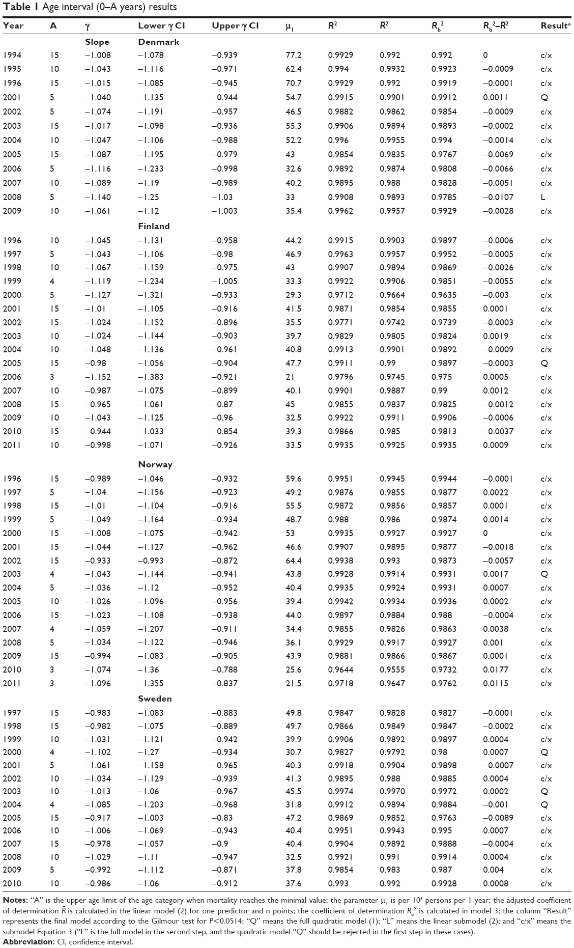Table 1 Age interval (0–A years) results Notes: “A” is the upper age limit of the age category when mortality reaches the minimal value; the parameter μ1 is per 105 persons per 1 year; the adjusted coefficient of determination is calculated in the linear model (2) for one predictor and n points; the coefficient of determination Rb2 is calculated in model 3; the column “Result” represents the final model according to the Gilmour test for P<0.0514; “Q” means the full quadratic model (1); “L” means the linear submodel (2); and “c/x” means the submodel Equation 3 (“L” is the full model in the second step, and the quadratic model “Q” should be rejected in the first step in these cases). Abbreviation: CI, confidence interval.

Results

Minimum of age–mortality trajectories

The first calendar year for Denmark, 1994, is shown as an example in Figure 3 in the log–log scale and also in Figure 4 in the semilogarithmic scale (the first calendar year for Norway is in Figures 1 and 2). Furthermore, the first and the last calendar year of every country are shown in odd-numbered figures (Figures S1, S3, S5, S7, S9, and S11) in the log–log scale and in even-numbered figures (Figures S2, S4, S6, S8, S10, and S12) in the semilogarithmic scale in the Supplementary materials.

Age trajectories from all diseases show a very strong minimum, which is hidden in total mortality. They have the minimal value in different age categories, and the upper age limit (A) of the specific age category in which mortality reaches the minimal value is shown in the second column in Table 1. Mortality from all diseases reaches the minimal value in three cases in the age category 2–3 years, in five cases in the age category 3–4 years, in 12 cases in the age category 4–5 years, in 18 cases in the age category 5–10 years, and in 20 cases in the age category 10–15 years. The mean of the ages where mortality from all diseases reached minimal value was 8 (95% confidence interval [CI] 7.05–8.95) years. Generally, the figures depict an age where the human population has minimal risk of death from biological causes.

Age trajectories of all-disease mortality have two evident parts, and the age axis is divided into two parts for further study in all cases. They are analyzed separately in the interval 0–A years and the interval A–95 years. The resulting age trajectories of mortality from all diseases show linear dependence before mortality minimum in the log–log scale in 0–A years in all calendar years and in all countries (Figures 1, 3, S1, S3, S5, S7, S9, and S11). Simultaneously, the nonlinear convex decline in the semilogarithmic scale is seen visually for all cases before the mortality minimum (Figures 2, 4, S2, S4, S6, S8, S10, and S12 in the semilogarithmic scale). Therefore, the linearity of age trajectories of all-disease mortality can be assumed in the log–log scale in the first interval of 0–A years.

On the other hand, linear age trajectories of mortality are found after the mortality minimum in the semilogarithmic scale in all cases in the second age interval (A–95 years) (Figures 2, 4, S2, S4, S, S8, S10, and S12 in the semilogarithmic scale). The approximate linear data of all-cause mortality and all-disease mortality correspond to the Gompertz exponential model. The model is shown as the straight line in the semilogarithmic scale in these figures. The data for all diseases and all causes are identical over the age of 40 years, while the data are already linear by age A for all diseases. This approximate linearity is seen in all cases.

Shape of age–mortality trajectory in the interval 0–A years

At first, the linearity in the log–log scale was tested in the following full model using the method of least squares (LS):

(1)

The null hypothesis H_o: δ =0 was not rejected in any cases (with two-sided P-values >0.05 in any country in any calendar year), while the slope γ was significant in all cases (two-sided P-values <0.05 in all cases). Consequently, the restricted linear model Equation 2 was assumed in all cases in the following step:

(2)

Two parameters, ln[μ₁] and γ, standard deviation of the parameters, and coefficient of determination R² in Equation 2 were calculated using LS in the age interval 0–A years. The residuals calculated in these two models in Denmark in all years are shown as examples (Figures S13 and S14). Similar random plots were confirmed in all other cases. The residuals calculated in these two models (Equations 1 and 2) were random in all cases, and the hypothesis that the residuals are not dependent on age in the log–log scale was not rejected for any cases (P>0.5). On the other hand, the residuals were strongly U-shaped in all cases for the linear model in the semilogarithmic scale, which corresponds to the exponential decrease with age (eg, Figure S15, where maximum and minimum of the y-axis are deliberately identical in three figures [S13–S15]).

Furthermore, two parameters, ln[μ₁] and γ, standard deviation of the parameters, and coefficient of determination R² in Equation 2 were calculated using LS, and the results are in Table 1. Coefficients of determination R² in Equation 2 were higher than 0.985 in 50 of 58 cases; the highest value was 0.9974 in Sweden in 2003 and the lowest 0.9644 in Norway in 2010.

Because all values of the slope γ were very close to −1, CI analysis was used to calculate 95% CIs for this slope. The null hypothesis Ho: γ = −1 in Equation 2 was not rejected in 54 of 58 cases (see all 95% CIs for parameter γ in Table 1). The specific value γ = −1 corresponds to the inverse proportion between mortality and age. If γ = −1, then it is valid:

(3)

The parameter μ₁ in Equation 3 can be simply estimated using LS. Generally, it is valid for n pairs of values ln[μ(x_i)] and ln(x_i):

(4)

and the logarithm of parameter μ₁ can be estimated in Equation 3 simply as the arithmetic mean:

(5)

Furthermore, the coefficient of determination R_b² in Equation 3 is

(6)

Resulting values of R_b² are in the ninth column in Table 1. Original values of R² in Equation 2 were recalculated with the adjusted coefficient of determination (for one predictor [ln(x)] and for n points here). The result values of are in the eighth column in Table 1, and they are close to the coefficients of determination R_b². The difference is in the next column, and R_b² was higher than in 27 of 58 cases.

Shape of age–mortality trajectory in the interval A–95 years

All cases were considered visually in the second age interval A–95 years, and age trajectories of mortality from all diseases were approximately linear in the semilogarithmic scale over age A (Figures 2, 4, S2, S4, S6, S8, S10, and S12). At first, the linearity in the semilogarithmic scale was tested in the following full model using LS in all cases:

(7)

The null hypothesis H_o: δ =0 was not rejected in Denmark in ten of 12 cases or seven of 16 cases in Finland (two-sided P>0.05). Parameter β was significant in all cases (two-sided P<0.05). Consequently, the age trajectory of mortality could be linear in these 17 cases in the semilogarithmic scale, and the following restricted equation was assumed:

(8)

This is the Gompertz model used for total mortality over 40 years.^{1,2,4–6,10,18,19,23,24} Two Gompertz parameters, ln[μ₀] and β, standard deviation of the parameters, coefficient of determination R², and adjusted coefficient of determination (for one predictor x) were calculated in Equation 8 using LS. The hypothesis that the residuals are not dependent on age in the semilogarithmic scale was not rejected for any cases (P>0.9 in all cases). The residuals calculated in the linear Equation 8 were random, and are shown for Denmark as an example in Figure S16. Similar plots are in all other 16 cases. The results calculated in Equation 8 are in the rows without values for parameter δ in Table 2.

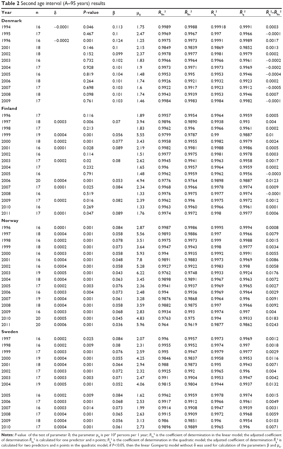Table 2 Second age interval (A–95 years) results Notes: P-value of the test of parameter δ; the parameter μ0 is per 105 persons per 1 year; Rlin2 is the coefficient of determination in the linear model; the adjusted coefficient of determination is calculated for one predictor and n points; Rq2 is the coefficient of determination in the quadratic model; the adjusted coefficient of determination is calculated for two predictors and n points in the quadratic model; if P<0.05, then the linear Gompertz model without δ was used for calculation of the parameters β and μ0.

The Gompertz model (Equation 8) fitted all age trajectories of all-disease mortality very well in these 17 cases. The values of adjusted coefficient of determination were between 0.9839 and 0.9983 (see the rows without parameter δ and the eighth column in Table 2). The parameter δ in the full nonlinear model (Equation 7) was significant in all other 41 cases (two-sided P<0.05). The three parameters ln[μ₀], β, and δ, standard deviation of the parameters, coefficient of determination R², and adjusted coefficient of determination (for two predictors – x and x) were calculated in the full model (Equation 7) using LS in the other two cases in Denmark, in the other nine cases in Finland, in all cases in Norway, and in all cases in Sweden (see the rows with values for parameter δ in Table 2). The residuals calculated in Equation 7 were random in these cases, and the hypothesis that the residuals are not dependent on age in the semilogarithmic scale was not rejected for any cases (two-sided P>0.05). The residuals calculated in the quadratic model (Equation 7) are shown for Sweden as an example in Figure S17, and similar plots are in all other 40 cases. The values of adjusted coefficient of determination were between 0.9862 and 0.9994 in these 41 cases (see the rows with parameter δ and the tenth column in Table 2).

Both adjusted coefficients of determination in model Equation 7 and in Equation 8 were calculated in all 58 cases, and their difference can be found in the last column in Table 2. The linear Gompertz model was better than the quadratic model in the semilogarithmic scale only in six cases in Denmark and in two cases in Finland, according to these differences.

Additions of the logistic model with two parameters and the Weibull model with two parameters are used in some studies, especially for other species.^25,26 The models were screened here, and parameters in the two models were calculated using LS in all cases. The residuals calculated in the Weibull model are shown for Denmark as an example in Figure S18, and similar plots were seen in all the other 57 cases. The maximum and minimum of the y-axis are deliberately identical in three figures (S16–S18). The two models should be excluded because the residuals are strongly U-shaped in all cases.

Discussion

Formal description of the shape of age trajectory from all diseases

If nonbiological causes are excluded from the spectrum of all causes, then the mortality minimum at age A divides age trajectories of mortality into two intervals. More detailed inspection of ages when mortality rate reaches the minimal value is given in Table S1. For example, the ages where mortality reached the minimal value were different in 1994 (Figure 3) and 2009 (Figure S1) for Denmark. The biggest difference within a single country is observed in Norway, where the age is 12.5 years in 1996 and 2.5 years in 2011. It is clear that explanation of this shift is not easy. The age trajectory of mortality is composed of two different parts, which lose their significance with age, and consequently the minimum is observed. The shift to lower ages of the minimum could be caused by lowering the first part of age trajectory after birth. Generally, this depends on both parts of the age–mortality trajectory, and if the first decreases the minimum goes to lower ages. On the other hand, if the second part of the age trajectory decreases, then the minimum goes to higher ages. The dynamics should be analyzed in other countries with different health systems.

The age trajectories were monotonic in both age intervals, and there was no reason to underline any smaller specific age interval for all diseases. For example, the age interval 15–40 years is very important for the shape of the age trajectory of total mortality where a typical hump is observed, which is caused by accidents.

The age interval 1–12 months has been selected by some authors as an important period after birth, but age trajectories of all diseases mortality show no dissimilarity in this age interval.^27–30 After birth, the simple model (Equation 3) fitted all-disease mortality very well. Other possible models mentioned in the literature were also tested here using LS in all cases. Initially, the Weibull distribution can generally describe linear mortality decline in the log–log scale. However, if mortality declines with a slope of −1 or less in the log–log scale, then the Weibull distribution is not applicable. The following definitions are valid for the Weibull cumulative distribution function F(x), for the survival function S(x), and for mortality rate μ(x):

(9)

The slope of the theoretical linear mortality decline in the log–log scale is m −1 here, where m and a are the Weibull parameters (formally, mortality rate μ₁ for x =1 is equal to m/a). This formalism could not be used for all-disease mortality, because the distribution was not defined for m ≤0 or for slope −1 (F[x] decreases with x, and could not be cumulative distribution function).

On the other hand, the analytic survival function S(x) could be derived using Equation 3 for x>x_min. For example, parameter x_min could be the first day of life (1/365 years) or the first hour of life (1/[365×24] years). It is valid:

(10)

Mortality decline with age after birth has been analyzed previously in the specific age interval 1–12 months.^27–30 These authors used the following Bourgeois-Pichat formula for cumulative deaths q(n) up to the age of n:

for 1 month ≤ n ≤12 months

(11)

Furthermore, Heligman and Pollard¹⁴ proposed the following relationship for mortality decline with age after birth:¹⁶

(12)

For illustration, the data in Norway in 1996 were fitted here by these two models. Parameters of Equations 11 and 12 were calculated using LS, and the resulting curves are shown in Figure 5. Notably, only two age categories, 7–28 days and 28–365 days, are used in Equation 11, while all age categories in the range of 0–10 years are used in Equation 12 (only two points are used for two parameters in Equation 11 here, which is extremely convenient to the model). However, the other two straight lines in Figure 5 are almost identical, corresponding to Equations 2 and 3 and parameters γ and μ₁ in Table 1.

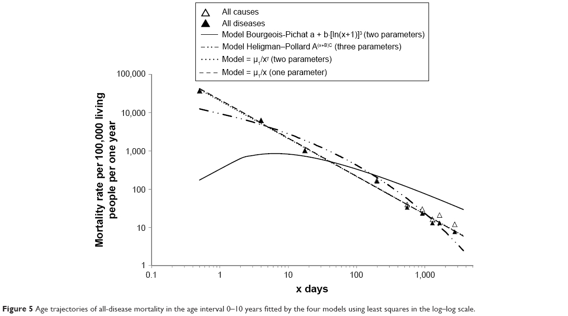Figure 5 Age trajectories of all-disease mortality in the age interval 0–10 years fitted by the four models using least squares in the log–log scale.

The results were similar in all other 57 cases in the Nordic countries. Equations 11 and 12 were not suitable in the interval 0–A years. Generally, Equation 3 differs from other mathematical formalisms useful in higher ages. These mortality dynamics could be explained by population heterogeneity. If individuals are characterized by individual congenital risks of death that are independent of age, then mortality rate represents a formal parallel to a mixture of radionuclides with different decay constants and mortality rate is similar to total radioactivity at the context. If these individual risks are approximately log-normally distributed at the moment of birth, then the population’s mortality could decrease with age, according to Equation 3. This has been numerically simulated in previous studies.^31,32 Furthermore, if the assumption that risks are log-normally distributed is replaced by the assumption that their density function f(r) is approximately constant (more severe impairments are less frequent), then the same theoretical mortality model (Equation 3) is obtained. The explanation also predicts that mortality rate could be independent of age for a population with smaller maximal individual risk, and simultaneously mortality could be inversely proportional to age in higher age categories (eg, for x >0.5–2 years). Empirical age trajectories of mortality calculated in more categories of diseases are actually constant during the first months, while they decrease as c/x in higher age categories.³¹

It has been shown in studies that age trajectories of total mortality can be concave in the semilogarithmic scale for x >40 years. Such nonlinearity is usually caused by slower mortality increase in higher ages (eg, some authors used the concave logistic model).^15,25 On the other hand, age trajectories from all-disease mortality were fitted here using the standard Gompertz model or the Gompertz model extended with a small positive quadratic term in age intervals A–95 years. The parameter δ in Equation 7, responsible for nonlinear increase in the semilogarithmic scale, was positive in all cases. For these reasons, age trajectories of all-disease mortality are moderately convex and with different curvature than total mortality. Furthermore, the Weibull and logistic models cannot be used after age A, because the residuals were strongly U-shaped and coefficients of determination were relatively low.

Possible clinical consequences

The distinction between biological and nonbiological causes of death is not completely clear in all situations. Observations realized in the paper are based on WHO definitions of cause of death and are mainly based on practical use of the definition. The distinction does not mean that among death listed in "biological" set the external causes have no significance (eg, smoking and lung cancer). On the other hand, it could mean that external factors (mainly accidents) are crucial to deaths listed in the nonbiological set. In other words, an individual without an accident event could be alive for more years. It is a model, and as with all models it has some limits. Age–mortality trajectories from all causes and all diseases were identical over 35 years. Consequently, the distinction between biological and nonbiological causes of death is not important over 35 years here. It is assumed that the distinction between the two categories of death cause could be clear under the age of 35 years.

Age could be ranked among the main factors that affect the risk of disease and the risk of death. Deaths before the age of 35 years are not usually assumed to be the result of aging. On the other hand, the two rare progeria syndromes – Werner’s syndrome and Hutchinson–Gilford progeria syndrome – represent two interesting exceptions.^33,34 Even before the age of 10 years, these two diseases represent extreme impairments, which could correspond to standard aging symptoms. Analysis of age–mortality trajectories shows that more clinical cases of death up the age of 35 years could be due to aging. The majority of cases after birth are related to congenital defects, but these causes gradually disappear with age (Table S1). Early manifestation of aging can be found in cardiovascular diseases or in other typical categories of mortality. The evidence that the shape of age trajectories from all-disease mortality is without any significant change after the age of 10 years shows that the mechanisms of aging could apply before the age of 35 years. Generally, specific disease could be the demonstration of aging, and disease could be only symptomatic of more essential processes. For example, according to Riggs’s “theory of competitive diseases”, there will never be a disappearance of the deceased patients of malignant neoplasms if general successful therapy is found. The realignment of these patients to other competitive diseases could be expected in such a situation.^2,35,36 For example, neurodegenerative diseases could represent such possible competitive diseases. Historically, the phenomenon was actually observed when antibiotics were successfully used in clinical practice and when mortality from infection diseases had dramatically declined. It has to be noted that the model was constructed for higher ages.

Population after birth and its heterogeneity

A first viewing of the age–mortality trajectory could lead to the assumption that the population is homogeneous (all people exhibit the same mechanisms of aging). On the other hand, more detailed inspection of the mortality spectrum shows that individuals differ significantly in their biological state. Consequently, the alternative assumption could be that the population is very heterogeneous. The second approach was used in frailty models of mortality.^37,38 Generally, aging itself could start earlier than age trajectories of mortality. It is discussed in some theories of aging, where the frailty index is used to describe differences in population with respect to individual risk of death. The difference between homogeneous and heterogeneous populations could be fundamental. A more theoretical discussion is undertaken in Vaupel et al.³⁷ An explanation of the shape of the age–mortality trajectory could be found in both homogeneous and heterogeneous populations. More empirical information could be found in the spectrum of death causes. Such information is simply projected in the classification of death here. The classification of death according to the WHO standard could also be burdened with some uncertainty. It could differ in different countries, in individual situations, etc. On the other hand, age of death represents the most reliable information. The application of the main classification categories in different ages is shown for Sweden in Table S2 (similar figures are valid in the other three countries). These shares of death could help to explain the mortality decline with age after birth. The majority of deaths up to 10 years are classified in the two categories “Certain conditions originating in the perinatal period” and “Congenital malformations, deformations, and chromosomal abnormalities”. The two categories are not practically used in adults. They show that the population of individuals dying at the first year could be very heterogeneous (about 85% of deaths are in the two categories). The situation is similar during the first 10 years (about 62% of deaths are in the two categories). In particular, congenital anomalies could represent a very different level of congenital impairment. Consequently, the shape of the age–mortality trajectory could be the result of the depletion of more impaired individuals.

The age–mortality trajectory is different after the mortality minimum, and simultaneously the mortality spectrum is also different. The category “Diseases of the circulatory system” is the most frequent over 10 years (46%), and neoplasms represent the second main category, with 26% (Table S2). Individual development in childhood represents an alternative explanation of the strong mortality decline with age after birth. Such explanation should take account the share of congenital anomalies and other impairments among cases up the age of 10 years.

The four countries represent a positive extreme around the world according to health care systems. The evidence could be significant here. Generally, it could be expected that the mortality spectrum in the age interval 0–35 years would be different in countries with worse health care systems. Consequently, all observations and conclusions should be confirmed or rejected in the other countries. Unfortunately, such studies could be limited by the quality of data. The WHO database does not usually contain suitable data of populations from the third world. The first four age categories should be used in the first year and 1-year categories up to the age of 5 years. For example, the WHO database does not contain relevant data for China or India.

Conclusion

The influence of nonbiological causes on age trajectories of all-cause mortality is crucial. It is especially visible within the age interval 5–30 years. The c/x model and the standard Gompertz model extended with a small positive quadratic term fit data on both sides of the mortality minimum. Life expectancy, which is one of the most important indicators and which could be used to quantify socioeconomic conditions, must be determined simultaneously by the two standard Gompertz parameters β and μ₀ and by the single parameter μ₁, which is a constant used in the inversion proportion between all-disease mortality and age after birth. The two categories “all diseases” and “nonbiological causes” are parallel and in principle different categories of death. Age trajectories of all-disease mortality represent an alternative tool to study the impact of age. All results shown in the study are based on published data. The results could be recalculated, and verified or rejected, with data from other populations.

Acknowledgments

This study was supported by the project Excellence 2017 and internal research at Faculty Informatics and Management, University of Hradec Kralove.

Disclosure

The authors report no conflicts of interest in this work.

---

References

1.		Gompertz B. On the nature of the function expressive of the law of human mortality. Philos Trans R Soc Lond. 1825;115:513–583.
2.		Strehler BL, Mildvan AS. General theory of mortality and aging. Science. 1960;132:14–21.
3.		Siler W. A competing risk model for animal mortality. Ecology. 1979;60:750–757.
4.		Witten MT. A return to time, cells, systems, and aging – V. Further thoughts on Gompertzian survival dynamics: the geriatric years. Mech Ageing Dev. 1988;46:175–200.
5.		Gavrilov LA, Gavrilova NS. The reliability theory of aging and longevity. J Theor Biol. 2001;213:527–545.
6.		Lin XS, Liu X. Markov aging process and phase-type law of mortality. N Am Actuar J. 2007;11:92–109.
7.		Arbeev KG, Ukraintseva SV, Akushevich I, et al. Age trajectories of physiological indices in relation to healthy life course. Mech Ageing Dev. 2011;132:93–102.
8.		Robine JM, Michel JP, Herrmann FR. Excess male mortality and age-specific mortality trajectories under different mortality conditions: a lesson from the heat wave of summer 2003. Mech Ageing Dev. 2012;133:378–386.
9.		Ukraintseva S, Yashin A, Arbeev K, et al. Puzzling role of genetic risk factors in human longevity: “risk alleles” as pro-longevity variants. Biogerontology. 2016;17:109–127.
10.		Luder HU. Onset of human aging estimated from hazard functions associated with various causes of death. Mech Ageing Dev. 1993;67:247–259.
11.		Dolejs J. The extension of Gompertz law’s validity. Mech Ageing Dev. 1997;99:233–244.
12.		Salinari G, De Santis G. On the beginning of mortality acceleration. Demography. 2015;52:39–60.
13.		Makeham W. On the law of mortality and the construction of annuity tables. J Inst Actuar. 1860;8:301–310.
14.		Heligman L, Pollard JH. The age pattern of mortality. J Inst Actuar. 1980;107:49–75.
15.		Vaupel JW, Carey JR, Christensen K, et al. Biodemographic trajectories of longevity. Science. 1998;280:855–860.
16.		Preston SH, Heuveline P, Guillot M. Demography: Measuring and Modeling Population Processes. Oxford: Blackwell; 2001.
17.		Bebbington M, Lai CD, Zitikis R. Modeling human mortality using mixtures of bathtub shaped failure distributions. J Theor Biol. 2007;245:528–538.
18.		Bebbington M, Lai CD, Zitikis R. Modelling deceleration in senescent mortality. Math Popul Stud. 2011;18:18–37.
19.		Willemse WJ, Koppelaar H. Knowledge elicitation of Gompertz’ law of mortality. Scand Actuar J. 2000;2:168–179.
20.		World Health Organization. Mortality, ICD-10. 2016. Available from: http://www.who.int/healthinfo/statistics/mortality_rawdata/en/index.html. Accessed January 27, 2015.
21.		World Health Organization. ICD-10: version 2010. Available from: http://apps.who.int/classifications/icd10/browse/2010/en. Accessed January 26, 2015.
22.		Eurostat. Population on 1 January by age and sex. 2016. Available from: http://appsso.eurostat.ec.europa.eu/nui/show.do?dataset=demo_pjan&lang=en. Accessed January 22, 2015.
23.		Zheng H, Yang Y, Land KC. Heterogeneity in the Strehler-Mildvan general theory of mortality and aging. Demography. 2011;48:267–290.
24.		Mulasso A, Roppolo M, Rabaglietti E. Physical frailty, disability, and dynamics in health perceptions: a preliminary mediation model. Clin Interv Aging. 2016:11:275–278.
25.		Wilson DL. The analysis of survival (mortality) data: fitting Gompertz, Weibull, and logistic functions. Mech Ageing Dev. 1994;74:15–33.
26.		Kesteloot H, Huang X. On the relationship between human all-cause mortality and age. Eur J Epidemiol. 2003;18:503–511.
27.		Bourgeois-Pichat J. De la mesure de la mortalité infantile. Population. 1946;1:53–68.
28.		Bourgeois-Pichat J. La mesure de la mortalité infantile II: les causes de déces. Population. 1951;6:459–480.
29.		Carnes BA, Olshansky SJ, Grahn D. The search for a law of mortality. Popul Dev Rev. 1996;22:231–264.
30.		Knodel J, Kintner H. The impact of breast feeding patterns on biometric analysis of infant mortality. Demography. 1977;14:391–409.
31.		Dolejs J. Analysis of mortality decline along with age and latent congenital defects. Mech Ageing Dev. 2003;124:679–696.
32.		Dolejs J. Decrease of total activity with time at long distances from a nuclear accident or explosion. Radiat Environ Biophys. 2005;44:41–49.
33.		Ding SL, Shen CY. Model of human aging: recent findings on Werner’s and Hutchinson-Gilford progeria syndromes. Clin Interv Aging. 2008;3:431–444.
34.		Coppedè F. The epidemiology of premature aging and associated comorbidities. Clin Interv Aging. 2013;8:1023–1032.
35.		Riggs JE, Millecchia RJ. Using the Gompertz-Strehler model of aging and mortality to explain mortality trends in industrialized countries. Mech Ageing Dev. 1992;65:217–228.
36.		Riggs JE. Rising mortality due to Parkinson’s disease and amyotrophic lateral sclerosis: a manifestation of the competitive nature of human mortality. J Clin Epidemiol. 1992;45:1007–1012.
37.		Vaupel JW, Manton KG, Stallard E. The impact of heterogeneity in individual frailty on the dynamics of mortality. Demography. 1979;16(3):439–454.
38.		Vaupel JW, Manton KG, Stallard E. The impact of heterogeneity in individual frailty on the dynamics of mortality. Demography. 1979;16:439–454.