Get the most from your data: a propensity score model comparison on real-life data

Introduction

Propensity score models are quite popular in modern clinical research practice. While the randomized clinical trial (RCT) is the method of choice when it comes to clinical studies, it might occur that they are not suitable or applicable for various reasons, eg, financing or ethics. In this case, one might perform a non-RCT to test a hypothesis.¹ Unfortunately, this study design can lead to heterogeneity in covariate distribution between two therapy groups, which makes it difficult to compare between the outcomes of therapy A versus B. Propensity score models are a simple tool to solve this problem and generate unbiased data.²

In 1983, Rosenbaum and Rubin introduced the propensity score as a new balancing score.² The propensity score unifies all known covariates from a patient in one score value between 0 and 1. Calculated by logistic regression, the propensity score is a patient’s likelihood of receiving a specific therapy, considering his or her covariates. Covariates in this context are actually all the characteristics a patient has, like blood type, weight, height, age, and sex, and also nonmedical aspects, such as education and leisure activities.^2,3 With the knowledge of all patients’ propensity scores, there are various ways to use them in further analysis. Common applications are nearest-neighbor matching and stratification.⁴ Nearest-neighbor matching, for instance, compares two individuals from separate groups with the most similar propensity score values in terms of their outcome. Patients without a match are dropped.

Since its introduction, there has been great discussion on which covariates should be considered in propensity score calculation, the calculation methods, the abilities and quality of propensity score results, and many other aspects of this tool. Stürmer et al⁵ argued that there is no factual evidence for superiority of the propensity score compared to traditional multivariate-outcome models. Hahn⁶ even claimed that the propensity score reduces the efficiency of outcome examinations. Bryson et al⁷ reduced the role of the propensity score to a simple average treatment-effect analysis method without further advantages. On the other hand, Cattaneo⁸ posited that propensity score models are superior to common multivariate-adjustment methods, especially when there are fewer than eight covariates included. However, in stating that there are legitimate reasons for using the propensity score, one might have a closer look at studies that examine more specialized and detailed applications in clinical research settings. Regularly used for binary-treatment comparisons, there are now approaches for multiple-treatment settings, as they are quite closer to reality, eg, when it comes to dose adaptation within a medical treatment group.⁹ Unfortunately, most propensity score evaluations are performed with Monte Carlo studies instead of real-life data.

One of the most critical issues in implementing propensity score analysis is the question of which covariates should be part of the model. While Rubin¹⁰ stated that propensity score models should be exhaustive and contain all available covariates, there are various voices against this procedure. Augurzky and Schmidt¹¹ supported Rubin’s thesis, claiming that this would lead to the true average treatment effect. As shown by Austin et al,¹² propensity score models based on outcome-relevant covariates might be a better tool. While models based on all covariates lead to a holistic propensity score, there is a significant reduction in matching pairs, because it becomes less probable to find a fitting match for a patient from group A in group B. Using just covariates that are significant within the logistic regression does not seem to be a suitable approach. Models based on this calculation are far too vague, even though one will find the lowest patient dropouts here. D’Agostino and D’Agostino¹³ also stated that there is clinical evidence to include these insignificant covariates.

Another aspect to consider is the choice of the best-fitting matching method. While Frölich¹⁴ could not find a significant difference in validity, Augurzky and Schmidt¹¹ showed that there is a significant loss of data due to patient dropout within nearest-neighbor matching, especially compared to stratification with quartiles. Furthermore, stratification would also lead to a reduced standard error. There are many more possibilities of matching methods, some of which were mentioned by Rosenbaum and Rubin,² like Mahalanobis or caliper matching. Those very special calculation methods are not part of this examination.

In respect of all those contrary arguments, the purpose of this study was to examine what kind of influence different propensity score models have on real non-RCT data and how they distinguish from one another in terms of outcome and data structure. Furthermore, we wanted to compare the outcome of this analysis to our native data and to findings in similar RCTs.

Materials and methods

Data

For our research purposes, we used a non-RCT by Otto et al.¹⁵ A total of 173 patients were recruited to compare the weight-loss effects of sleeve gastrectomy versus Roux-en-Y gastric bypass; 127 patients decided to receive bypass surgery, and 46 patients received sleeve gastrectomy. To become part of this study, patients had to be older than 18 years and fulfill the criteria of body mass index (BMI) >40 kg/m² or BMI >35 kg/m² in combination with comorbidity.

In general, patients could choose between both therapy options, but there was a clear recommendation for sleeve gastrectomy with patients who suffered from gastroesophageal reflux disease, psychiatric diseases, who needed dialysis, or had a BMI >60 kg/m².

The surgical procedure was performed with a standard technique and laparoscopically. Roux-en-Y gastric bypass was applied with an antecolic Roux limb of 150 cm and a 50 cm biliopancreatic limb. For the sleeve gastrectomy, the calibration of the gastric sleeve was done with a 42-French bougie, inserted along the lesser gastric curvature. Linear stapling went from 5 cm proximal to the pylorus to the angle of Hiss. In cases of bleeding or inadequate staples, the stapling line got oversewn.

Follow-up was performed in an outpatient clinic after 6 weeks, 18 weeks, 6 months, 9 months, and 12 months. For comparison, presurgical baselines were measured 1 day before the intervention. Measured data included body composition using the bioelectrical impedance-analysis tool Nutriguard-MS (Data Input GmbH, Darmstadt, Germany) and Nutri Plus software. The relevant criterion for this study was excess weight loss (EWL). EWL is defined as the percentage loss of overweight. We performed native statistic analysis with SAS version 9.3 (SAS Institute Inc, Cary, NC, USA).

Propensity score analysis

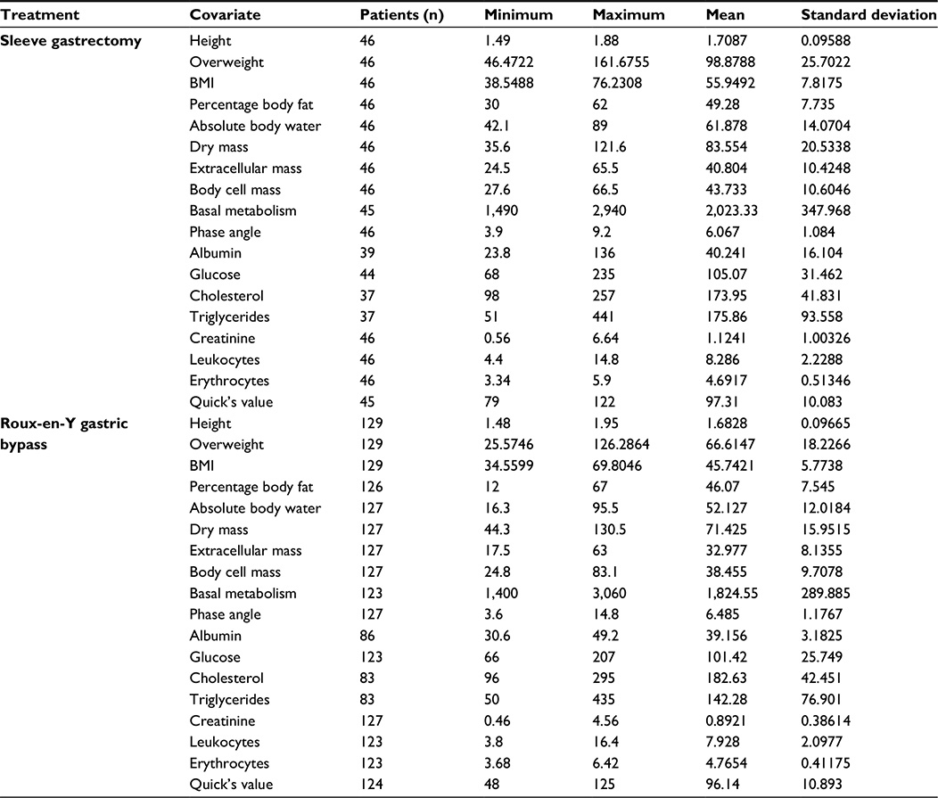
In a first step in order to perform propensity score analysis, we checked both therapy groups for heterogeneity within the distribution of their covariates, specifically their sex, height, overweight, BMI, percentage body fat, absolute body water, dry mass, extracellular mass, body cell mass, basal metabolism, phase angle, albumin, glucose, cholesterol, triglycerides, creatinine, leukocytes, erythrocytes, and Quick’s value. For this purpose, we used Mann–Whitney U tests and the χ² test. Given the native data, we also performed two-sample t-tests with all relevant EWL percentages.

Afterward, we defined three different propensity score models that we used for statistical analysis. These three models were based on the most popular ways to choose included covariates. The first model contained just outcome-related covariates, and the second model was based on all covariates in order to calculate an exhaustive score. The third model contained just significant covariates in logistic regression. Within this analysis, we defined significance as P<0.05. We identified outcome-related covariates by reviewing current scientific publications and discussion with bariatric surgeons. This model included sex, overweight, BMI, percentage body fat, body cell mass, basal metabolism, phase angle, glucose, and creatinine. Calculation of the exhaustive propensity score includes sex, height, overweight, BMI, percentage body fat, absolute body water, dry mass, extracellular mass, body cell mass, basal metabolism, phase angle, albumin, glucose, cholesterol, triglycerides, creatinine, leukocytes, erythrocytes, and Quick’s value.^16–22 To identify significant covariates, we used logistic regression with backward elimination. Therefore, we used BMI and creatinine as the covariates of choice.

Using the defined propensity score models, we performed a logistic regression to calculate propensity score values for each patient and each model. Knowing these values, we started the matching procedure. In respect of the recent discussion on the best method of data adjustment with propensity scores, we decided to perform nearest-neighbor matching with a maximum difference of 5% in propensity scores between both matching partners and stratification by quartiles.

After propensity score adjustment, we checked both therapy groups again for heterogeneity in covariates with Mann–Whitney U tests and performed two-sample t-tests for every model and adjustment procedure to examine the difference in mean EWL. We performed all statistical analysis with SPSS version 22 for Mac OS X (IBM, Armonk, NY, USA).

Results

Native data

Student’s t-test (Table 1) proved that there was a significant difference in EWL between the therapy groups after 18 weeks and 1 year. As emphasized earlier, one has to consider heterogeneity within the groups’ covariate distribution. Mann–Whitney U tests and χ² testing indicated that the groups contained an unequal distribution for the following covariates, as shown in Table 2: overweight, BMI, percentage body fat, absolute body water, dry mass, extracellular mass, body cell mass, basal metabolism, phase angle, and triglycerides. The P-value of the χ² test for the distribution of sex was 0.174.

Table 1 Student’s t-test for mean differences in native data Abbreviations: EWL, excess weight loss; BMI, body mass index.

Table 2 Comparison between both therapy groups Abbreviation: BMI, body mass index.

Propensity score analysis with
significant covariates

This model led to an outcome comparison between 54 patients: 27 matching pairs. The mean propensity score for sleeve gastrectomy was 0.4442 and for Roux-en-Y gastric bypass was 0.8391. Values in parentheses are minima and maxima. After the matching procedure had been performed, mean values were 0.5691 (0.029–0.9571) for sleeve gastrectomy and 0.5802 (0.0191-0.9668) for Roux-en-Y gastric bypass (Table 3). Table 4 shows that heterogeneous distribution in covariates was reduced to leukocytes. Student’s t-tests for mean differences in EWL showed no significant difference between the groups after matching.

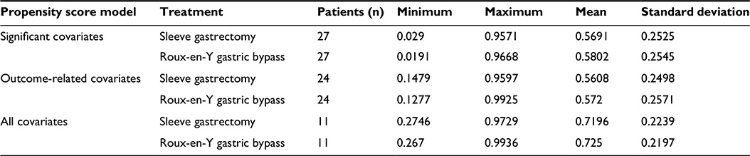Table 3 Propensity score comparison after matching

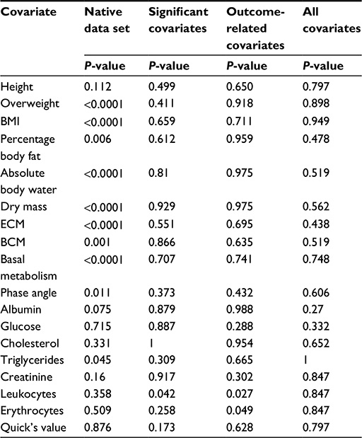Table 4 Mann–Whitney U tests Abbreviations: BMI, body mass index; ECM, extracellular mass; BCM, body cell mass.

Propensity score analysis with outcome-related covariates

Containing 48 patients, or 24 matching pairs, this model led to a mean propensity score of 0.3976 for sleeve gastrectomy and 0.8539 for Roux-en-Y gastric bypass before we performed matching. Afterward, these values were 0.5608 (0.1479–0.9593) and 0.572 (0.1277–0.9925) (Table 3). Unequally distributed covariates remained within the number of leukocytes and erythrocytes. Again, t-tests for mean EWL between the therapy groups showed no significant difference.

Propensity score analysis with all covariates

With the highest loss of data, this model contained 22 patients in eleven matching pairs. Mean propensity score values before matching were 0.2991 for sleeve gastrectomy and 0.8526 for Roux-en-Y gastric bypass. Compared to our other models, this was the biggest difference between mean propensity scores, which also indicated relevant heterogeneity in covariate distribution between the therapy groups. After our matching procedure, these values adapted to 0.7196 (0.2476–0.9729) for sleeve gastrectomy and 0.725 (0.267–0.9936) for Roux-en-Y gastric bypass (Table 3). The exhaustive propensity score model was the only one without any residual observed heterogeneously distributed covariate. As seen earlier, the t-test for mean propensity score values showed no significant difference for EWL.

Summary

In contrast to our native data, which contained significant heterogeneity in covariate distribution, all propensity score models led to the result that there was actually no significant difference in EWL between sleeve gastrectomy and Roux-en-Y gastric bypass. This conclusion is similar to the findings of Peterli et al,²³ who performed an RCT to examine the weight loss between these therapy options. The outcome within all propensity score models based on non-RCT was equal to the results of an actual RCT, while the native non-RCT analysis showed a significant difference.

Differences within our models were seen in their ability to eliminate heterogeneity in covariate distribution and the loss of data. Residual heterogeneous distribution in covariate distribution might still be a reason for confounding, but is very unlikely, especially when using propensity score calculation with outcome-related covariates. Within other models, it is necessary to discuss their effect on the outcome. The more covariates we included in the models, the fewer the residual heterogeneous covariates, but the larger the loss of data in terms of matching dropouts. It seems adequate to balance both effects by including just covariates that might have an effect on the observed outcome. Therefore, it is necessary to emphasize preclinical preparation as an important consideration in planning a non-RCT if one wants to include propensity score analysis. Reviewing literature and discussing pathophysiologic pathways, which might affect the outcome beyond medical aspects, are the main points in forming the best-fitting propensity score model.

This scheme for organizing a non-RCT with propensity score analysis is shown in Figure 1. We marked sections that have to receive special attention when it comes to propensity score matching. To calculate adequate propensity scores, one needs to identify all outcome-related covariates. Reviewing actual research literature and discussing extramedical aspects must be emphasized. Also, data collection during the first patient contact in a prestudy setting and during the clinical study needs to be focused. Only with a reliable and holistic data set is there a chance to compare both therapy groups as objectively as possible.

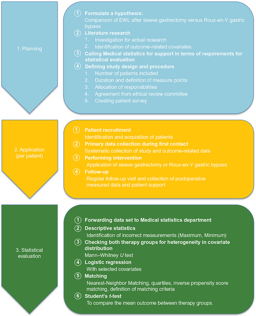Figure 1 Suggestion for an optimized clinical trial procedure including propensity score matching. Abbreviation: EWL, excess weight loss

In conclusion, we showed that there is no need to apply highly specialized statistical methods for reliable calculations, as recent literature often might imply. The key advantage of propensity score analysis is its simplicity if adequate preparation is done.

Discussion

Our work proved that propensity score analysis is actually able to eliminate heterogeneity within covariate distribution in patients of non-RCTs. Nevertheless, one needs to consider the impact of dropouts on the P-value. With rising standard deviation and decreasing sample size, the t-test is more likely to be significant. Due to this possible bias, it is necessary to interpret these findings in a holistic statistical analysis. Therefore, it might be useful to plan future studies with an increased number of patients. In our case, we accepted this because of our predetermined limited resources and an additional clinical consideration of our data afterward. We did not observe critical issues in terms of propensity score usage. Some former studies implied that these might occur within choosing the right covariates or comparative tests. It just seems to be important to prepare statistical analysis with meticulous data collection and perform a holistic selection for outcome-related covariates. As seen in our work, propensity score models based on all available covariates led to absolute homogeneous covariate distribution but were accompanied by a tremendous loss of data. A useful trade-off we chose was propensity score calculation based on outcome-related covariates. Residual heterogeneous distributions should be critically examined for their influence on the study. Our data showed a remaining imbalance between the therapy groups in respect to their amounts leukocytes and erythrocytes. There is actually no reason to see an impact of these factors on EWL. Observed patient dropouts in the outcome-related propensity score model stood in a rational connection to bias reduction. Concerning patient dropouts, one might argue that patients without matches referring to their extreme propensity score values also do not reflect the regular potential target audience for the specific therapy, which narrows the influence of this loss of data.

A definite advantage of this work lies within the holistic comparison of various propensity score models on a real-life database. Earlier works often focused on specific and very complex statistical procedures while using Monte Carlo data sets. Furthermore, this work emphasized the central role of data collection, which is the key aspect when it comes to reliable propensity score analysis.

Also, with regard to keeping data as native as possible, we did not use oversampling for our calculations. Oversampling uses a patient various times as matching partner for different members of the other therapy group. We decided to stay as near to a natural study environment as possible. Methodologically, we were restricted, as we had to work with a preexisting non-RCT. Therefore, we had no influence on data collection. Also, we analyzed mean differences for EWL with t-tests and did not use tools like inverse probability of treatment weighting using the propensity scores or caliper analysis. These advanced statistical methods seemed not suitable for our goal of proving the efficiency and simplicity of propensity score models.

Unfortunately, we only had the capacity to perform these calculations with one study. For further examination, it would be very interesting to analyze these simple propensity score implementations for a wide range of non-RCTs. By doing so, we might get a deeper understanding of chances going along with propensity score matching, and it might appear that these simple models especially are the perfect match for non-RCT analysis. Talking about validating and establishing propensity scores in statistical examinations, we also have to ask whether there is a necessity to perform RCTs. From an ethical and economical point of view, there are a lot of arguments against RCTs, like their higher organizational effort and difficult recruitment of patients. Of course, there is no way to simulate natural conditions as perfectly as appears in a RCT, but as in every other aspect of science, we should consider tools like propensity scores a valuable compromise. By doing so, it seems suitable to set a standardized framework for propensity score analysis in terms of covariate selection and matching procedures in regard to comparability and transparency.

Acknowledgments

The authors developed this study in cooperation with Dr Mirko Otto from the Department of General Surgery at University Medical Center Mannheim, Dr Marc Schmittner from the Department of Anesthesia, and with the supervision of Professor Christel Weiss, chief of the Department for Medical Statistics and Biomathematics. This work is part of the doctoral research of Dennis Ferdinand, student and MD candidate at the University of Heidelberg.

Disclosure

The authors report no conflicts of interest in this work.

References

1.		Dannehl K. Experimental study versus non-experimental study: the non-experimental (non-randomized) study as a methodological compromise. In: Abel U, Koch A, editors. Nonrandomized Comparative Clinical Studies. Düsseldorf: Symposion; 1998:41–52.
2.		Rosenbaum PR, Rubin DB. The central role of the propensity score in observational studies for causal effects. Biometrika. 1983;70(1):41–55.
3.		Brookhart MA, Schneeweiss S, Rothman KJ, Glynn RJ, Avorn J, Stürmer T. Variable selection for propensity score models. Am J Epidemiol. 2006;163(12):1149–1156.
4.		Rubin DB, Thomas N. Matching using estimated propensity scores: relating theory to practice. Biometrics. 1996;52(1):249–264.
5.		Stürmer T, Joshi M, Glynn RJ, Avorn J, Rothman KJ, Schneeweiss S. A review of the application of propensity score methods yielded increasing use, advantages in specific settings, but not substantially different estimates compared with conventional multivariable methods. J Clin Epidemiol. 2006;59(5):437–447.
6.		Hahn J. On the role of the propensity score in efficient semiparametric estimation of average treatment effects. Econometrica. 1998;66(2):315–331.
7.		Bryson A, Dorsett R, Purdon S. The Use of Propensity Score Matching in the Evaluation of Active Labour Market Policies. London: Department for Work and Pensions; 2002.
8.		Cattaneo MD. Efficient semiparametric estimation of multi-valued treatment effects under ignorability. J Econom. 2010;155(2):138–154.
9.		Feng P, Zhou XH, Zou QM, Fan MY, Li XS. Generalized propensity score for estimating the average treatment effect of multiple treatments. Stat Med. 2012;31(7):681–697.
10.		Rubin DB. Estimating causal effects from large data sets using propensity scores. Ann Intern Med. 1997;127(8 Pt 2):757–763.
11.		Augurzky B, Schmidt CM. The propensity score: a means to an end. 2001. Available from: http://papers.ssrn.com/sol3/papers.cfm?abstract_id=270919. Accessed April 5, 2016.
12.		Austin PC, Grootendorst P, Anderson GM. A comparison of the ability of different propensity score models to balance measured variables between treated and untreated subjects: a Monte Carlo study. Stat Med. 2007;26:734–753.
13.		D’Agostino RB Jr, D’Agostino RB Sr. Estimating treatment effects using observational data. JAMA. 2007;297(3):314–316.
14.		Frölich M. Finite-sample properties of propensity score matching and weighting estimators. Rev Econ Stat. 2004;86(1):77–90.
15.		Otto M, Elrefai M, Krammer J, Weiss C, Kienle P, Hasenberg T. Sleeve gastrectomy and Roux-en-Y gastric bypass lead to comparable changes in body composition after adjustment for initial body mass index. Obes Surg. 2016;26(3):479–485.
16.		Chagnac A, Weinstein T, Herman M, Hirsh J, Gafter U, Ori Y. The effects of weight loss on renal function in patients with severe obesity. J Am Soc Nephrol. 2003;14(6):1480–1486.
17.		Cottam DR, Schaefer PA, Shaftan GW, Velcu L, Angus LD. Effect of surgically-induced weight loss on leukocyte indicators of chronic inflammation in morbid obesity. Obes Surg. 2002;12(3):335–342.
18.		Folsom AR, Qamhieh HT, Wing RR, et al. Impact of weight loss on plasminogen activator inhibitor (PAI-1), factor VII, and other hemostatic factors in moderately overweight adults. Arterioscler Thromb. 1993;13(2):162–169.
19.		Kyle UG, Genton L, Pichard C. Low phase angle determined by bioelectrical impedance analysis is associated with malnutrition and nutritional risk at hospital admission. Clin Nutr. 2013;32(2):294–299.
20.		Layman DK, Boileau RA, Erickson DJ, et al. A reduced ratio of dietary carbohydrate to protein improves body composition and blood lipid profiles during weight loss in adult women. J Nutr. 2003;133(2): 411–417.
21.		Norman K, Stobäus N, Pirlich M, Bosy-Westphal A. Bioelectrical phase angle and impedance vector analysis – clinical relevance and applicability of impedance parameters. Clin Nutr. 2012;31(6):854–861.
22.		Pelleymounter MA, Cullen MJ, Baker MB, et al. Effects of the obese gene product on body weight regulation in ob/ob mice. Science. 1995;269(5223):540–543.
23.		Peterli R, Borbély Y, Kern B, et al. Early results of the Swiss Multicentre Bypass or Sleeve Study (SM-BOSS): a prospective randomized trial comparing laparoscopic sleeve gastrectomy and Roux-en-Y gastric bypass. Ann Surg. 2013;258(5):690–695.