Back to Journals » Clinical Epidemiology » Volume 14
Considerations for Using Multiple Imputation in Propensity Score-Weighted Analysis – A Tutorial with Applied Example
Authors Eiset AH ![]() , Frydenberg M
, Frydenberg M
Received 23 December 2021
Accepted for publication 3 June 2022
Published 7 July 2022 Volume 2022:14 Pages 835—847
DOI https://doi.org/10.2147/CLEP.S354733
Checked for plagiarism Yes
Review by Single anonymous peer review
Peer reviewer comments 4
Editor who approved publication: Professor Henrik Toft Sørensen
Andreas Halgreen Eiset,1,2 Morten Frydenberg3
1Department of Affective Disorders, Aarhus University Hospital–Psychiatry, Aarhus, Denmark; 2Department of Public Health, Aarhus University, Aarhus, Denmark; 3Consultant Biostatistician, Independent, Trige, Denmark
Correspondence: Andreas Halgreen Eiset, Department of Affective Disorders, Aarhus University Hospital–Psychiatry, Palle Juul-Jensens Boulevard 175, Aarhus N, 8200, Denmark, Tel +45 7847 2450, Email [email protected]
Purpose: Propensity score-weighting for confounder control and multiple imputation to counter missing data are both widely used methods in epidemiological research. Combination of the two is not trivial and requires a number of decisions to produce valid inference. In this tutorial, we outline the assumptions underlying each of the methods, present our considerations in combining the two, discuss the methodological and practical implications of our choices and briefly point to alternatives. Throughout we apply the theory to a research project about post-traumatic stress disorder in Syrian refugees.
Patients and Methods: We detail how we used logistic regression-based propensity scores to produce “standardized mortality ratio”-weights and Substantive Model Compatible-Full Conditional Specification for multiple imputation of missing data to get the estimate of association. Finally, a percentile confidence interval was produced by bootstrapping.
Results: A simple propensity score model with weight truncation at 1st and 99th percentile obtained acceptable balance on all covariates and was chosen as our model. Due to computational issues in the multiple imputation, two levels of one of the substantive model covariates and two levels of one of the auxiliary covariates were collapsed. This slightly modified propensity score model was the substantive model in the SMC-FCS multiple imputation, and regression models were set up for all partially observed covariates. We set the number of imputations to 10 and number of iterations to 40. We produced 999 bootstrap estimates to compute the 95-percentile confidence interval.
Conclusion: Combining propensity score-weighting and multiple imputation is not a trivial task. We present considerations necessary to do so, realizing it is demanding in terms of both workload and computational time; however, we do not consider the former a drawback: it makes some of the underlying assumptions explicit and the latter may be a nuisance that will diminish with faster computers and better implementations.
Keywords: observational studies, multiple imputation, propensity score weighting, bootstrap confidence interval, tutorial
Introduction
In this paper we present the considerations behind estimating the change in prevalence of post-traumatic stress disorder (PTSD) associated with long-distance migration using multiple imputation to handle missing data, propensity score-weighting to adjust for confounding, and bootstrap to produce a percentile confidence interval.
The propensity score is the probability of exposure (E) given a relevant set of covariates (V),  . Let
. Let  be the estimated propensity score for individual i then the “standardized mortality ratio weights”,
  , may be used to estimate the association between long-distance migration and PTSD by subtracting the weighted average of the prevalence of PTSD among refugees who migrated to Lebanon from the prevalence among those who migrated to Denmark. This requires a number of decisions including: Which covariates should be included in the propensity score model? What level of complexity should be modeled? How can extreme weights be dealt with? And how to calculate the standard error of the parameter of interest? As we had missing data in the covariates and in PTSD status, we set out to combine the propensity score-weighted analysis with multiple imputation. This raised additional questions such as: What are the required assumptions of the missing data process? What is the substantial model and which variables should be included in the model? How can multiple imputation be combined with propensity score analysis? How to find a valid confidence interval for the parameter of interest?
In this tutorial we discuss the implementation of the planned analysis and focus on the many statistical methodological problems we encountered recognizing that alternative choices and methods may be appropriate in other settings. The reader is referred to the applied paper1 for the subject matter problem. The relevant data consisted of a 20-item questionnaire and a clinical examination including assessment of possible psychiatric disorders, applied to a sample of Syrian asylum seekers in Denmark and a sample of Syrian refugees in Lebanon. The outcome, PTSD, was assessed using the “Harvard Trauma Questionnaire” part IV,2 giving a score from 1 to 4 with 2.5 the commonly used cut-off-score for PTSD.
In the following subsections, we outline the problems we had to consider and the underlying theory. In the Methods section, we discuss our considerations on how to implement these in our specific study and in the Results section, we provide details on our final implementation. The problems, theory, considerations and decisions are summarized in Tables 1, 2 and 3.
 |
Table 1 Considerations and Decision for Building the Propensity Score Model |
 |
Table 2 Considerations and Decision for Building the Multiple Imputation Model |
 |
Table 3 Consideration and Decision for Combining Multiple Imputation and Propensity Score-Weighting and Obtaining Valid Confidence Interval |
The Propensity Score Analysis
Table 1 provides an overview of the considerations and decisions for building the propensity score model. The relevant predictors to be included in the propensity score model are covariates that (potentially) confound the relationship between exposure and outcome. The outcome itself should never be included in the model and, according to some studies, variables that are only associated with the exposure may increase the uncertainty around the estimate without decreasing bias.3,4 The complexity of the regression model should be chosen so that all covariate distributions are balanced between exposure groups indicating successful confounding adjustment.5,6 In a propensity score-weighted analysis, the desired weights are used in a weighted analysis giving the estimate of association, and the confidence interval can be produced by applying some approximate formula to obtain a standard error or via bootstrapping.7,8 Extreme weights may lead to suboptimal covariate balance and unstable estimates.9 This problem is most often remedied by smoothing or truncation at the cost of potentially introducing bias.10
Missing Data
The statistical properties of many missing data methods rely on the hypothesized missingness mechanism. The primary interest in applied epidemiology, is whether the missing data mechanism is ignorable, that is, if valid inference can be drawn despite missing data. In many applied papers using multiple imputations (MI) the authors state that the data are “missing at random” and “as a consequence” the inference based on MI is valid. We will briefly consider the definition and importance of “missing data” drawing primarily on Seaman et al.11 Very loosely speaking, data are “missing at random”, if the risk of a data point being missing only depends on the observed data. The terminology “missing at random” (MAR) and “missing completely at random” (MCAR, which imply MAR) has been in use at least since Rubin’s 1976 paper12 and was recently extended to include “realized” and “everywhere” versions of both MAR and MCAR by Seaman et al.11 In the latter paper the definition is based on parametric models for both the data, Z, (which includes both the outcome variable, Y, and covariates, X) and the missingness indicator vector, M, (which for each entry in z, specify if it is observed). Note that we do not observe the entire z, but only the entries, where the corresponding entry in m is 1 and we let  denote the observed part of the data, z. Furthermore we let
  denote the density for the data and
  the conditional probability of the missing pattern, m, given the data z, with the parameters
  . In a specific study we have the realized data
  and missing indicator vector
  with the realized observed data
  .
.
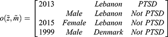
Example 1. Consider a very small data set with four refugees and four variables: “year of residency”, “sex”, “host country”, and “PTSD-status”. One realization could be:
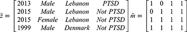
Data are said to be realized-MAR if for all  ,
,  for all z, where
  that is, the probability of the realized missingness pattern
  is the same for all data z that has an observed part that is identical to the realized observed data, that is, the unobserved part is of no interest. In Example 1, the data are realized-MAR, if the conditional probability that data on “sex” for observation number 1 and data on “year of residency” for observation number 2 are missing and all other entries are observed, does not depend on the value of the missing sex and year of residency as long as all the observed entries are as realized. This is a statement that focuses only on the realized missingness pattern and the realized observed data; we do not consider other possible missingness patterns or other possible realizations of the data. To emphasize: it is irrelevant whether for instance “sex” on observation number 2 or “country” on observation number 3 could be missing.
Data are everywhere-MAR if the data are realized-MAR for all possible realizations and not only for the actually observed realization of the missingness pattern and data. That is, for any missingness pattern, m, and any two realizations of Z, z and  , where the observed part is identical,
  , we have the same probability for the missing pattern
  . Returning to Example 1, when assuming everywhere-MAR the realized data set is irrelevant: we must check the whole set of possibly missing data conditional probabilities,
  for all parameter values,
  .
.
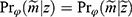
The above elaborations were necessary to qualify the question of interest: Is the missingness mechanism ignorable? That is, when can we make valid inference about the parameter of interest,  , based only on the observed data? Seaman et al11 illustrated that the answer depends on the type of statistical inference framework and in the “frequentist likelihood framework” the missingness mechanism must be everywhere-MAR (and the parameters
  , be variation independent, ie,
  ). Therefore, in order to ignore the missingness mechanism in our applied example we must argue that it is reasonable to assume everywhere-MAR. This implies that, for all possible missingness patterns and corresponding observed data, it is reasonable to assume that the risk of that specific pattern does not depend on the value of the missing data but only on the observed data. This is of course an impossible task without some insight into why data are missing in the study. One way to start off is to assume that the missing data mechanism is identical and works independently from person to person, which reduces the problem to a discussion of the mechanism for a single person.
For example, in Example 1, we have no missing in “PTSD” in the realized observed data, however, we can easily imagine this information missing in another realization of the study. If we assume identical and independent missing mechanism, we have to think of why “year of residency”, “sex”, and “PTSD” could be missing for a person and if the risk of this is independent of the unobserved values given what we have observed for that person. For example, if we only observe “country”, we have to argue, that the risk of this missingness pattern is the same for all individuals in each country, ie, it does not depend on year, sex or whether or not the person has PTSD. We note that the assumption of independent missingness mechanism might easily be invalid, for example missingness could depend on some unobserved event common for several persons in the study.
Multiple Imputations
In the following, we will assume that the purpose of the data analysis is to estimate  , typically a vector of regression coefficients based on the proposed model for the analysis of interest—ie, the substantive model—of Y given the covariates X:
Many statistical methods assume no missing data or missingness mechanism MCAR and will produce biased estimates otherwise.13 A popular way to deal with missing data is to use multiple imputation which gives unbiased estimates assuming ignorable missingness mechanism and correctly specified multiple imputation model.14,15 Table 2 gives an overview of the considerations and decisions for using multiple imputation to deal with missing data. Briefly, multiple imputation consists of producing a number, K, of data sets with imputed values for the missing data and analyze these complete data sets as planned, resulting in K estimates of  which are combined, typically by taking the average, into a final estimate for
  16 When implemented, the imputation is done for each variable with missing data (a) specifying a regression model for the conditional distribution of the variable given the other (relevant) variables, (b) using the observed data to estimate the parameters in this model, (c) impute the missing values of the variable by simulating from the Bayesian posterior predictive distribution. The last two steps will in general be taken care of by a software program, as long as the imputation regression models are chosen within the most common regression model families. Often, several of the variables in the imputation regression model will have missing values, resulting in a so-called “chained equation”, that is, the imputed values in one variable are needed to impute the values in another variable and vice versa. Luckily, many software packages can solve this problem using iterative methods. Thus, after deciding on what implementation of multiple imputation to use we are left with problem (a): How to specify the imputation regression models, ie, what should be used as the substantive model in the multiple imputation, what variables to include in the multiple imputation models and how many iterations must be run between sampling? It has been known for a while that bias may be introduced in the estimation of
  , if the multiple imputation models are not carefully specified.13,17 This can happen if the relationship between the outcome y and x in the substantive model is more complicated than the relationship between x and y in the implemented imputation regression models. For example, if y is not included in the imputation regression model for the covariate
  then the imputed data for
  will be unrelated to y resulting in an underestimate of the regression coefficient
  relating y to
  in the substantive model. Furthermore, if
  and
and  interact in the substantive model for y, then y and
  should (at least) interact in the imputation model for
  to avoid bias in the estimate of the magnitude of the interaction. It is difficult, even for relatively simple substantive models, to determine how to specify the imputation models in order to avoid this problem. Luckily there exists a statistical method that can combine a specification of the substantive regression model, y on x, with univariate regression models for each of the variables in x given the rest of the x’s, into an imputation algorithm. Details about this method, the Substantive Model Compatible-Full Conditional Specification (SMC-FCS) multiple imputation, is given in Bartlett et al’s work16 and the algorithm has been implemented in R and Stata for a set of standard regression models.18,19 As the SMC-FCS algorithm is an iterative algorithm, it will not generate independent samples which implies that one cannot use subsequent samples but only use samples with a specific interval between them. The estimate of interest is found by averaging the estimates from each imputed data set (“Rubin’s rules”).20 The confidence interval must take into account the uncertainty introduced by modeling the missing data, for example using Rubin’s variance estimator or bootstrapping.20–23
Bootstrapping
Table 3 gives an overview of the considerations and decision combining propensity score-weighting and multiple imputation and obtaining a valid confidence interval. Non-parametric bootstrapping is a method to find an approximate confidence interval for a parameter, when applying a specific estimation algorithm to a data set. In bootstrapping the only input is the data set and the estimation algorithm and no assumption is made concerning the distribution or the estimation algorithm.24 However, the realized sample is assumed to be independent and representative of the target population.25 In the simple bootstrap, the estimation algorithm is applied to the original data and to a number of bootstrap samples, that is, artificial data sets with the same number of observations as the original, but with the observations being sampled randomly with replacement from the original data set. This results in the original estimate and a set of bootstrap estimates from which a 95% confidence interval can be produced as (a) the original estimate ± 1.96 times the standard deviation of the bootstrap estimates or (b) the 2.5th and 97.5th percentile of the bootstrap estimates. The first strategy typically requires a relatively small number of bootstrap samples, but rely on approximate normality of the estimates, while the second strategy requires a large number of bootstrap samples but does not make any assumptions about the distribution of the estimates.
Materials and Methods
Based on the theoretical considerations detailed above, we will outline our estimation algorithm as illustrated in Figure 1. The analysis plan was defined a priori and included a number of decisions:
- the exposure (long-distance migration), outcome (PTSD) and potential confounders (age, sex, socioeconomic status, experienced trauma, and mental well-being).
- addressing of confounding by logistic regression-based propensity score modeling and of missing data by multiple imputation.
- the complexity of the regression model for the propensity score model was determined by exploring covariate balance for different plausible models.
- given ignorable missingness mechanism, multiple imputation of the missing data was performed using the SMC-FCS algorithm with the chosen propensity score model as the substantive model
- for each of the multiple imputed data sets: the propensity scores were computed using the chosen propensity score model, converted into weights and the weighted point estimates produced
- the mean of the point estimates produced in step 5) was the estimate of interest
- the 95 percentile confidence interval was produced by bootstrapping steps 4–6 a large number of times.
 |
Figure 1 Flow-chart of proposed methodology to combine multiple imputation and propensity score weighting. In the example, a full line represents an observed value for the given observation and variable, no line represents a missing value and a dotted line represents a multiple imputed value. The original data set is multiple imputed and the propensity score-weighted estimate is computed for each complete data set. These estimates are averaged to produce the point estimate. The 95% confidence interval is computed by bootstrapping a large number, R (eg 999), of data sets, ie, sampling with replacement from the observations. The entire procedure in the magnifying glass is repeated for each of the bootstrap data sets and the 2.5th and 97.5 percentiles are used as the lower and upper limits. *Each of the sampled bootstrap data sets are used in place of the original data set. |
The Propensity Score Model
In propensity score modeling, covariate balance between the two exposure groups is a measure of confounder control. Here, balance was defined as an absolute standardized mean difference of ≤ 0.10 between the exposure groups for all covariates.26 Three plausible propensity score models of increasing complexity were defined (“simple”, “intermediate”, and “complex”) and three levels of weight truncation (no truncation, truncating at the 1st and 99th percentile, or truncating at the 5th and 95th percentile) were examined for covariate balance.5,26 Based on a single imputed data set for each of the three complexities, the least complex model with the least amount of truncation to obtain acceptable balance, was chosen for the analysis. See the Supplementary Data 1 and the first author’s GitHub page (https://github.com/eiset/ARCH) for details of the specific models and the exploratory plots.
The Multiple Imputation Model
It should be noted that the existing implementation of the SMC-FCS algorithm does not cover our substantive model, the propensity score-weighted analysis, consequently, we decided to use the model for the propensity score as our substantive model. For each partially observed covariate we specified a “prediction model”, meaning a regression model to predict the missing value of the partly observed covariate (the response in the regression model in question) given the PTSD score and any additional covariates as deemed relevant based on subject matter insight and exploratory plots. When entering as the response variable, all continuous partially observed covariates were modeled using linear regression with relevant transformation and all discrete covariates were modeled using logistic, multinomial or proportional odds regression. When entering as “predictor variables”, all continuous covariates were modeled as restricted cubic splines with knots at the 10th, 50th and 90th percentiles; all discrete covariates and interactions entered unaltered (see Supplementary Data 1). The sampling interval between the imputations was decided based on plots of the parameter estimates against the sampling interval.
The Estimate of Association and Its Confidence Interval
The “within” procedure was implemented to combine propensity score-weighting and multiple imputation:27,28 a number of data sets were imputed and for each data set the prevalence difference of PTSD according to long-distance migration was estimated and averaged to give the point estimate (“impute, compute, combine”). The 95-percentile confidence interval was found by bootstrapping this procedure, ie, repeating the previously mentioned steps (4-6) 999 times: resampling a new data set with missing data, performing multiple imputation and producing the propensity score-weighted estimate. The procedure is illustrated in Figure 1.
All data management, analysis and plots were done in R29 with heavy reliance on packages “smcfcs”18 for SMC-FCS multiple imputation; “WeightIt”30 and “cobalt”31 for estimation of propensity score weights and assessment of covariate balance; “boot”32 for parallelized bootstrapping; “furrr”33 for further parallelizing procedures; and “tidyverse” packages34 for data wrangling and plotting. The code was run on two Ubuntu systems (18.04.5 and 20.04.1) and a Windows 10 system; all running R 4.0.3. The analysis plan and all R codes for analysis and plots, including the specific settings in each procedure are available from the first author’s GitHub page (https://github.com/eiset/ARCH).
Results
The simple propensity score model with weight truncation at 1st and 99th percentile obtained acceptable balance for all covariates and was chosen as our model. Unfortunately, but not surprisingly, we had to modify our first choice of substantive model (ie, the propensity score model used in the imputation) due to computational/numerical problems by collapsing two levels of one of the substantive model covariates and two levels of one of the auxiliary covariates.
This slightly modified propensity score model was the substantive model in the SMC-FCS multiple imputation and regression models were set up for all partially observed covariates: for example, for imputing the continuous covariate “Age”, the logarithmic transformation of Age, “log Age”, was modeled with covariates from the substantive model entering as “predictor variables”: “Socioeconomic status”, “PTSD” (as restricted cubic spline) and auxiliary regressors: “Highest education”, “Number of children”, “Systolic blood pressure” (as restricted cubic spline), and “Marital status”. The Age variable was then passively imputed from “log Age” by exponentiating. All partially observed auxiliary variables were also imputed. The “predictor matrix” in the Supplementary Data 1 gives details on models for all partly observed variables.
We set the number of imputations to 10 which is well beyond what is often considered sufficient.35 The convergence plots showed that a sampling interval between imputations, ie, iterations, of 20 was sufficient; to err on the safe side, we chose 40 iterations. Following recommendations of Carpenter and Bithell,25 we produced 999 bootstrap estimates to compute the 95-percentile confidence interval. For practical reasons, three different computers were used to run the final analysis. The time to run 250 bootstrap estimates was from two to 10 hours depending on the system.
In the applied example, the analysis showed an increased prevalence amounting to 8.76 percentage points (95-percentile confidence interval [−1.39; 18.62 percentage points]) with little variation in the sensitivity analysis. We refer to the accompanying paper for discussions of the results.1
Discussion
In this paper we describe the statistical methodological considerations for combining propensity score-weighting for confounder control and multiple imputation of missing data. In the following, we will discuss the assumptions behind both propensity score-weighted estimation and multiple imputation and their combination.
The Propensity Score-Weighting
Model misspecification is considered the overarching source of bias in propensity score modeling.10,36 In our approach, the propensity score model of interest and covariates to be included were explicit and based on the available evidence and subject matter knowledge, however, we recognize the possibility of some remaining bias, for example from residual confounding and from the collapsing of two levels of one of the variables. It has been suggested that machine learning or “black box” algorithms may provide reasonable propensity score-weights,10,37,38 however, at the cost of control over the model. Extreme weights were truncated as advocated by several,5,7,10 acknowledging that the decrease in variance comes at the cost of possibly introducing bias. Stabilized weights is another approach to decrease the variance but comes at a similar cost;6 a recent paper7 found that when estimating the hazard rate by propensity score-weighted Cox regression, the choice between ordinary propensity score-weighting (in this case using weights to produce the “average treatment effect”) or its stabilized version made no difference on the confidence interval coverage and that bootstrap gave the least biased variance estimates with best confidence interval coverage.
The Multiple Imputation
The substantive model of interest was the propensity score model. It was explicitly specified which is paramount in fulfilling one of the assumptions of multiple imputation: a correctly specified substantive model of interest. For the researchers, this may be an additional undertaking compared to automated “black box” algorithms, however, as Bartlett et al noted “We do not consider the requirement to specify a substantive model at the imputation stage to be a shortcoming … ”.16 The SMC-FCS algorithm allows defining the substantive model of interest and imputation models for each partially observed variable and takes care of combining these in the multiple univariate imputations. This may increase the possibility to correctly specify the multiple imputation model.10,36 Recent studies suggest, however, that misspecification of the multiple imputation model may not be detrimental in obtaining valid percentile confidence interval when applying a methodology as proposed in this paper.20 Another assumption of multiple imputation is the ignorable missingness mechanism. In the applied example we subjected every variable to careful examination and are satisfied that the “everywhere-MAR” assumption was not violated, however, we acknowledge that this is subject to discussion and cannot be guaranteed. Also, we did not consider multiple imputation of the missing data separately for groups that may differ in important ways such as for each exposure group. In theory, separate models may reduce bias in the imputed data sets, however, in the applied example we abstained from this due to sparse data.
The Estimate of Association and Its Confidence Interval
Seaman and White22 showed that the “within” procedure as proposed by Qu and Lipkovich39 and implemented in the present tutorial gives an unbiased point estimate assuming correctly specified propensity score model and ignorable missingness mechanism. We used bootstrap to produce a 95-percentile confidence interval. There is no clear evidence on what step to bootstrap when combining propensity score-weighting and multiple imputation.21 In our approach, we bootstrapped the entire “within” procedure to produce a confidence interval that accounts for all uncertainty introduced by modeling in both the propensity score and multiple imputation step. This procedure is similar to that applied to a simple simulated data set by Penning de Vries and Groenwold.28 Schomaker and Heumann21 suggested that bootstrapping after multiple imputing the data sets may produce similar results at lower computational expense, however, a later study20 found that this may increase bias compared with bootstrapping the entire procedure. Alternatively, “Rubin’s rule” is used in several studies and is the traditional choice when doing multiple imputation (without propensity score modeling). Qu and Lipkovich39 noted that “Rubin’s rule” does not account for the uncertainty introduced in the propensity score estimation and, thus, is not valid in theory while others note that it may produce valid estimates in practice.22 Our proposed methodology takes several hours to run on “standard” laptop computers and we experienced numerical problems with strata with relatively few observations. Going forward, we are eager to examine the sensitivity of our result to different methodologies for example using other g-methods such as g-computation or other multiple imputation methods such as machine learning algorithms. The produced point estimate and confidence interval could also be compared to alternative methods that lower the computing time such as “Rubin’s rules” or the recently proposed “von Hippel” method for using bootstrap in multiple imputation (though does not include propensity score modeling).40
Conclusion
In this article we have striven to make clear the many choices that we had to go through to combine propensity score-weighting and multiple imputation. While both approaches are commonly used in many research settings, their combination is not straight forward and require careful attention to the specification of each method and their combination. It is our hope that others can make use of our experience in planning their research, creating the analysis plan, and running their analysis.
Abbreviations
MAR, missing-at-random; MCAR, missing-completely-at-random; MI, multiple imputation; PTSD, post-traumatic stress disorder; SMC-FCS, Substantive Model Compatible-Full Conditional Specification.
Code Availability
The analysis plan and all R codes for the applied example are available from https://github.com/eiset/ARCH.
Author Contributions
All authors made a significant contribution to the work reported, whether that is in the conception, study design, execution, acquisition of data, analysis and interpretation, or in all these areas; took part in drafting, revising or critically reviewing the article; gave final approval of the version to be published; have agreed on the journal to which the article has been submitted; and agree to be accountable for all aspects of the work.
Funding
The authors did not receive support from any organisation for the submitted work.
Disclosure
The authors report no conflicts of interest in this work.
References
1. Eiset AH, Aoun MP, Stougaard M, et al. The association between long-distance migration and PTSD prevalence in Syrian refugees. BMC Psychiatry. 2022;22:363. doi:10.1186/s12888-022-03982-4
2. Mollica RF, Caspi-Yavin Y, Bollini P, Truong T, Tor S, Lavelle JW. The Harvard Trauma Questionnaire: validating a cross-cultural instrument for measuring torture, trauma, and posttraumatic stress disorder in Indochinese refugees. J Nerv. 1992;180(2):111–116. doi:10.1097/00005053-199202000-00008
3. Brookhart MA, Schneeweiss S, Rothman KJ, Glynn RJ, Avorn J, Stürmer T. Variable selection for propensity score models. Am J Epidemiol. 2006;163(12):1149–1156. doi:10.1093/aje/kwj149
4. Austin PC. An introduction to propensity score methods for reducing the effects of confounding in observational studies. Multivar Behav Res. 2011;46(3):399–424. doi:10.1080/00273171.2011.568786
5. Austin PC, Stuart EA. Moving towards best practice when using inverse probability of treatment weighting (IPTW) using the propensity score to estimate causal treatment effects in observational studies. Stat Med. 2015;34(28):3661–3679. doi:10.1002/sim.6607
6. Cole SR, Hernán MA. Constructing inverse probability weights for marginal structural models. Am J Epidemiol. 2008;168(6):656–664. doi:10.1093/aje/kwn164
7. Austin PC. Variance estimation when using inverse probability of treatment weighting (IPTW) with survival analysis. Stat Med. 2016;35(30):5642–5655. doi:10.1002/sim.7084
8. Chan KCG, Yam SCP, Zhang Z. Globally efficient non-parametric inference of average treatment effects by empirical balancing calibration weighting. J R Stat Soc Ser B Stat Methodol. 2016;78(3):673–700. doi:10.1111/rssb.12129
9. Robins JM, Hernán MA, Brumback B. Marginal structural models and causal inference in epidemiology. Epidemiol Camb Mass. 2000;11(5):550–560. doi:10.1097/00001648-200009000-00011
10. Lee BK, Lessler J, Stuart EA. Weight trimming and propensity score weighting. PLoS One. 2011;6(3):e18174. doi:10.1371/journal.pone.0018174
11. Seaman SR, Galati J, Jackson D, Carlin J. What is meant by “missing at random”? Stat Sci. 2013;28(2):257–268. doi:10.1214/13-STS415
12. Rubin DB. Inference and missing data. Biometrika. 1976;63(3):581–592. doi:10.2307/2335739
13. Little RJA. Regression with Missing X’s: a review. J Am Stat Assoc. 1992;87(420):1227–1237. doi:10.2307/2290664
14. Rubin DB. Multiple imputation after 18+ years. J Am Stat Assoc. 1996;91(434):473–489. doi:10.2307/2291635
15. Sterne JAC, White IR, Carlin JB, et al. Multiple imputation for missing data in epidemiological and clinical research: potential and pitfalls. BMJ. 2009;338:b2393–b2393. doi:10.1136/bmj.b2393
16. Bartlett JW, Seaman SR, White IR, Carpenter JR. Multiple imputation of covariates by fully conditional specification: accommodating the substantive model. Stat Methods Med Res. 2015;24(4):462–487. doi:10.1177/0962280214521348
17. Seaman SR, Bartlett JW, White IR. Multiple imputation of missing covariates with non-linear effects and interactions: an evaluation of statistical methods. BMC Med Res Methodol. 2012;12:46. doi:10.1186/1471-2288-12-46
18. Bartlett JW, Keogh R Smcfcs: multiple imputation of covariates by substantive model compatible fully conditional specification.; 2020. https://CRAN.R-project.org/package=smcfcs.
19. Bartlett JW, Morris TP. Multiple imputation of covariates by substantive-model compatible fully conditional specification. Stata J Promot Commun Stat Stata. 2015;15(2):437–456. doi:10.1177/1536867X1501500206
20. Bartlett JW, Hughes RA. Bootstrap inference for multiple imputation under uncongeniality and misspecification. Stat Methods Med Res. 2020;29:3533–3546. doi:10.1177/0962280220932189
21. Schomaker M, Heumann C. Bootstrap inference when using multiple imputation. Stat Med. 2018;37(14):2252–2266. doi:10.1002/sim.7654
22. Seaman SR, White I. Inverse probability weighting with missing predictors of treatment assignment or missingness. Commun Stat - Theory Methods. 2014;43(16):3499–3515. doi:10.1080/03610926.2012.700371
23. Murray JS. Multiple imputation: a review of practical and theoretical findings. Stat Sci. 2018;33(2):142–159. doi:10.1214/18-STS644
24. Efron B. Bootstrap methods: another look at the jackknife. Ann Stat. 1979;7(1):1–26. doi:10.1214/aos/1176344552
25. Carpenter J, Bithell J. Bootstrap confidence intervals: when, which, what? A practical guide for medical statisticians. Stat Med. 2000;19(9):1141–1164. doi:10.1002/(SICI)1097-0258(20000515)19:9<1141::
26. Austin PC. Balance diagnostics for comparing the distribution of baseline covariates between treatment groups in propensity-score matched samples. Stat Med. 2009;28(25):3083–3107. doi:10.1002/sim.3697
27. Leyrat C, Seaman SR, White IR, et al. Propensity score analysis with partially observed covariates: how should multiple imputation be used? Stat Methods Med Res. 2019;28(1):3–19. doi:10.1177/0962280217713032
28. Penning de Vries BBL, Groenwold RH. A comparison of two approaches to implementing propensity score methods following multiple imputation. Epidemiol Biostat Public Health. 2017;14(4). doi:10.2427/12630
29. R Core Team. R: a language and environment for statistical computing. R Foundation for Statistical Computing; 2020. Available from: http://www.R-project.org/.
30. Greifer N WeightIt: weighting for covariate balance in observational studies; 2020. Available from: https://CRAN.R-project.org/package=WeightIt.
31. Greifer N Cobalt: covariate balance tables and plots; 2020. Available from: https://CRAN.R-project.org/package=cobalt.
32. Canty A, Ripley B Boot: bootstrap R (S-Plus) functions; 2020.
33. Vaughan D, Dancho M Furrr: apply mapping functions in parallel using futures.; 2020. Available from: https://CRAN.R-project.org/package=furrr.
34. Wickham H, Averick M, Bryan J, et al. Welcome to the Tidyverse. J Open Source Softw. 2019;4(43):1686. doi:10.21105/joss.01686
35. Harrell F. Regression Modeling Strategies: With Applications to Linear Models, Logistic and Ordinal Regression, and Survival Analysis.
36. Austin PC, Stuart EA. The performance of inverse probability of treatment weighting and full matching on the propensity score in the presence of model misspecification when estimating the effect of treatment on survival outcomes. Stat Methods Med Res. 2017;26:1654–1670.
37. Bahamyirou A, Blais L, Forget A, Schnitzer ME. Understanding and diagnosing the potential for bias when using machine learning methods with doubly robust causal estimators. Stat Methods Med Res. 2019;28(6):1637–1650. doi:10.1177/0962280218772065
38. Penning de Vries BBL, Smeden M, Van Groenwold RHH. Propensity score estimation using classification and regression trees in the presence of missing covariate data. Epidemiol Med. 2018;7(1). doi:10.1515/em-2017-0020
39. Qu Y, Lipkovich I. Propensity score estimation with missing values using a multiple imputation missingness pattern (MIMP) approach. Stat Med. 2009;28(9):1402–1414. doi:10.1002/sim.3549
40. von Hippel PT, Bartlett JW. Maximum likelihood multiple imputation: faster imputations and consistent standard errors without posterior draws. ArXiv12100870 Stat. 2019;36:400–420.
 © 2022 The Author(s). This work is published and licensed by Dove Medical Press Limited. The
full terms of this license are available at https://www.dovepress.com/terms
and incorporate the Creative Commons Attribution
- Non Commercial (unported, 3.0) License.
By accessing the work you hereby accept the Terms. Non-commercial uses of the work are permitted
without any further permission from Dove Medical Press Limited, provided the work is properly
attributed. For permission for commercial use of this work, please see paragraphs 4.2 and 5 of our Terms.
© 2022 The Author(s). This work is published and licensed by Dove Medical Press Limited. The
full terms of this license are available at https://www.dovepress.com/terms
and incorporate the Creative Commons Attribution
- Non Commercial (unported, 3.0) License.
By accessing the work you hereby accept the Terms. Non-commercial uses of the work are permitted
without any further permission from Dove Medical Press Limited, provided the work is properly
attributed. For permission for commercial use of this work, please see paragraphs 4.2 and 5 of our Terms.