Back to Archived Journals » Open Access Bioinformatics » Volume 8
Computational advances applied to medical image processing: an update
Authors Joao A, Gambaruto A, Tiago J, Sequeira A
Received 25 August 2015
Accepted for publication 22 January 2016
Published 29 March 2016 Volume 2016:8 Pages 1—15
DOI https://doi.org/10.2147/OAB.S70327
Checked for plagiarism Yes
Review by Single anonymous peer review
Peer reviewer comments 3
Editor who approved publication: Professor Alex MacKerell
Ana João,1 Alberto M Gambaruto,2 Jorge Tiago,1 Adélia Sequeira1
1Center for Computational and Stochastic Mathematics, Instituto Superior Técnico, Universidade de Lisboa, Lisbon, Portugal; 2Department of Mechanical Engineering, University of Bristol, Bristol, UK
Abstract: Medical imaging provides a high-fidelity, noninvasive, or minimally invasive means for effective diagnostic and routine checks, and has become an established tool in both clinical and research settings. The interpretation of medical images commonly requires analysis by an experienced individual with the necessary skills. This dependence on an individual's evaluation in part limits the broader scope and widespread use of medical images that would be possible if performed automatically. The analysis of medical images by an individual may also influence reliability, with different users attaining alternative conclusions from the data set. It is thus beneficial to support the experienced user with robust and fast processing of the medical images for further analysis that relies as little as possible on user interaction. In the existing body of literature, a variety of methods have been proposed for medical image filtering and enhancement, which have been largely used in the context of improving image quality for both human visual perception and feature detection and object segmentation via a numerical algorithm. In this study, an analysis of some popular methodologies for image processing is presented. From the comparison of results, a robust and automatic pipeline procedure for medical image processing is put forward, and results for different imaging-acquisition techniques are given.
Keywords: medical imaging, automatic image processing, image filtering, contrast enhancement, object segmentation, feature extraction
Introduction
The rapid increase in and immense potential of noninvasive medical imaging and data-acquisition techniques has fueled research in mathematical modeling for medical image processing. Of specific interest are robust and automatic methods that can provide repeatability in results, as well as high quality of desired processing. A usual goal in image analysis is the extraction of important detail or features in an image data set for subsequent evaluation, which is typically achieved by segmentation, hence the delineation of the desired object contour. Other common processing steps for medical images that have attracted much attention are those of filtering noise, contrast enhancement, bias correction, and registration. Each processing step aims to support and facilitate any subsequent analysis that is part of a procedural pipeline compared to the unprocessed image.
Methods based on partial differential equations have been keenly studied for image filtering (smoothing), due to their success in reducing noise while preserving important image structures. Linear isotropic diffusion is a widely used method for image filtering, and in practice involves the convolution of a Gaussian function (Green’s function of the diffusion equation) with the image.1 As such, linear isotropic diffusion is often referred to as Gaussian smoothing (or filtering). While this is simple and effective, edge blurring and dislocation are among the known downfalls of the approach that limit its use. Nonlinear anisotropic diffusion, introduced by Perona and Malik2 in image processing, overcomes the downfalls of Gaussian filtering by being spatially adaptive depending on the local properties of the image, such as the image gradient. The method as proposed by Perona and Malik2 has been reported to suffer from numerical instabilities, resulting in a “staircasing” effect, which is when a mild-gradient region evolves piecewise into almost linear segments separated by jumps. As a result, several approaches have been proposed for regularization of the method in an attempt to overcome the ill-posed nature of the problem and attain desirable results.3-5
In a medical setting, it is often the case that the acquired images suffer from low contrast, which may ultimately affect the accuracy of analysis and diagnosis. Contrast enhancement of an image is therefore of critical interest. Choosing an appropriate contrast-enhancement method is not straightforward, due to lack of dependable measures that quantify the quality of the output image. A variety of methods have been proposed in the literature, and are either based on a frequency representation of the image or employ the spatial information of the scene directly. In this work, popular methods belonging to both representations are adopted. Specifically, the discrete cosine transform (DCT) contrast-enhancement method is employed as an example of frequency-based methods, while the unsharp masking (UM) and local histogram equalization (HE) methods are investigated and belong to the spatial representation methods.
Image segmentation and edge detection are arguably the most important image-processing tasks. The extraction of important features of an image is still a challenging problem, and several segmentation algorithms have been proposed over the decades. Segmentation methods rely on partitioning the image into sets of homogeneous regions so that the pixels in each region carry congruent characteristics. The methods may be built on different underlying assumptions of how to interpret the information present in an image, and result in making use of various parameters, such as grayscale level, texture, color, or motion. Medical image segmentation is usually performed based on the grayscale values, based on two different approaches: by detecting discontinuities or through association by similarity. The latter includes segmenting the image based on the similarity of the intensity between neighboring pixels within a given region, while the former resorts to identifying sudden changes in the grayscale values. Accurate, robust, and automatic segmentation methods for medical images are keenly sought, in order to facilitate and improve patient data-set analysis and clinical evaluation.
While the attention of this study is the postprocessing of images once they have been acquired from the scanning machines, it is relevant to mention the preprocessing methods employed by these scanners to generate the output medical image data set. There are two major in-reconstruction techniques: analytical reconstruction and iterative reconstruction.
Analytical methods are strongly influenced by the choice of reconstruction kernel. This kernel defines a tradeoff between the presence of noise and the spatial resolution.6 Sharp kernels generate images with high spatial resolution (eg, commonly used for bone-structure diagnosis), while a smooth kernel produces images with low noise and reduced spatial resolution (eg, commonly used for brain, breast, or liver tumors). Other parameters, such as slice thickness, also play an important role in imaging quality, as this controls the spatial resolution in the longitudinal direction, influencing the balance between image resolution, noise, and radiation dose.7
On the other hand, iterative reconstruction techniques use prior knowledge of the image or noise statistics. An example of this technique is the maximum likelihood reconstruction method, which estimates an image from projections by maximizing the log likelihood of the acquired data (computed tomography, magnetic resonance imaging, and positron-emission tomography data). Since this may result in very noisy images, a penalty function or a termination threshold is used as a regularization. Ideally, a regularization function is able to preserve spatial smoothing within a region and sharp transition of region boundaries.8
When acquisition techniques are not sufficient or result in low-quality images, postprocessing methods may be needed. Considering possible limitations and with the aforementioned image-processing principles and objectives in mind, it is beneficial to combine all the processing steps needed and implement an automatic and robust pipeline for an image-processing algorithm that would help clinicians to process patient data. To overcome the hurdle of arduous and lengthy data processing, tests, and calculations, the whole pipeline from medical image acquisition to segmentation should be fully optimized with the target of reducing or downright eliminating manual intervention and decision making. The selection of optimal parameters and methodologies is done through a set of well-known image-quality metrics, which include an estimator for the mean squared error (MSE), a measure for contrast-to-noise ratio (CNR), and a structural similarity (SSIM) metric, all widely used in the image-processing community.
A threefold pipeline of techniques for image processing is suggested: image denoising while preserving the edges, contrast enhancement, and region-of-interest segmentation. An in depth comparison of different regularizations of the anisotropic filters that rely on spatial derivatives is also described. With the aim of providing a pipeline with broad applicability, data sets obtained from different medical imaging modalities are considered in this study. Nevertheless, we cannot expect the approach to be robust or optimal for all possible cases. For clarity, representative images from each data-set stack are presented, in order to explain both processing stage and results.
Image data sets and quality metrics
Three data sets of medical images obtained from different image-acquisition modalities, as detailed herein, are studied to ensure effectiveness and the broad scope of the image-processing methods. In doing so, we attempt to account for the various noise types and artifacts that arise in the different imaging modalities. Additionally, the effects of the image-processing steps are examined by adopting a set of image-quality metrics, as detailed herein. Such metrics are individually limited in scope; however, combined they provide a general basis for gauging the extent of improvement or deterioration in a processed image with respect to the raw image.
Image data sets
A representative image from each data set is chosen and extensively investigated for each of the image-processing methods considered. The selected images are considered as matrices I(x, y) of dimension (1, nx)×(1, ny), hence the x-axis is aligned to the row index and the y-axis to the column index. The total number of pixels is nx·ny, and the grayscale intensity is normalized to the range 0–255. Note that after any processing the scale is restored to the same range. For brevity, the images are denoted by I and subscripts used to provide information of the image processing performed, if any. For example, the raw unprocessed image is referred to as Iorig, to denote it is the original. The medical image data sets used in this work are:
- computed tomography angiography (cerebral aneurysm): comprising 194 images in the axial plane, with spatial resolution 512×512, pixel size 0.26×0.26 mm, 0.6 mm slice thickness, and 1 mm slice spacing; image 74 of this data set is shown in the first row of Figure 1
- magnetic resonance imaging (brain): comprising 276 images in the axial plane, with spatial resolution 512×512, pixel size 0.48×0.48 mm, 0.62 mm slice thickness, and 1 mm slice spacing; the magnetization-prepared rapid-acquisition gradient echo sequence was used; image 76 of this data set is shown in the second row of Figure 1
- computed tomography (nasal cavity): comprising 276 images in the axial plane, with spatial resolution 512×512, pixel size 0.49×0.49 mm, 0.59 mm slice thickness, and 1 mm slice spacing; image 94 of this data set is shown in Figure 1.
 | Figure 1 Image data sets used. |
Image-quality metrics
Presenting the quality of an image by a set of quantifiable measures ensures a repeatable and unambiguous analysis. Such measures are commonly referred to as image-quality metrics, and additionally serve to adapt and tune processing- algorithm parameters to obtain excellent results. An ideal-quality metric would mimic the human visual system, being a measure of the effective interpretation and analysis of the image by any given individual. Unfortunately, since the visual system itself is highly complex and still not fully understood, most existing metrics are designed based on simplifying assumptions. Additionally to these metrics, specific properties of medical images should be preserved during the processing, especially the localization of object boundaries, as these are of evident clinical interest.
Specifically, we are concerned with measuring the result of the image processing based on the following three criteria:
- reduction of noise
- image quality based on image comparison
- object-edge preservation.
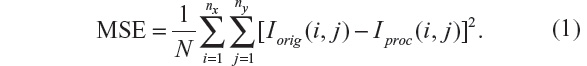
A simple and widely used measure is the MSE, calculated by averaging the squared intensity differences between the Iorig and processed image (Iproc):
Related measures, such as the peak signal-to-noise ratio (PSNR) and signal-to-MSE ratio are means of normalizing the MSE measure. Another popular measure in image processing is the CNR, which is given by:
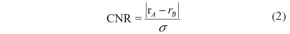
where rA and rB are signal intensities for the region of interest and noise, respectively, and σ is the standard deviation of the image noise.
These measures are appealing due to their simplicity, ease of calculation, and clear physical meaning; however, they undoubtedly lack visual quality perception. To complement these, the SSIM is also considered, which is based on the hypothesis that the human visual system is deeply adapted for extracting structural information.9
The SSIM is given by:
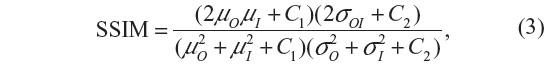
where μO, μI denote the average and σO, σI are the standard deviation of the grayscale intensities of the original and processed image, respectively, and σOI is the covariance of the original image and processed image. C1 and C2 are constants that avoid instabilities when μO2 + μI2 is close to zero.
Filtering methods
The filtered image is a function of time as I(x, y, t) solution, where t denotes the incremental time step in the process. The general nonlinear anisotropic (nonhomogeneous) diffusion process looks for the solution of:
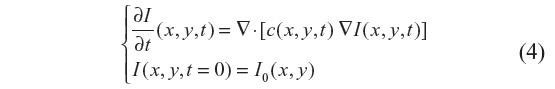
where ▽· and ▽ represent the divergence and gradient operators respectively, and c(x, y, t) is the diffusion coefficient. Equation 4 is discretized using an explicit forward-in-time finite-difference scheme, which reads:

where Δh and ▽h are the discrete Laplace and gradient operators, while the superscripts indicate the time-integration steps.
All the filtering methods detailed from here rely on Equation 4, with different forms of the diffusion coefficient c(x, y, t). In the case of the nonlinear complex-diffusion despeckling filter (NCDF) method, an adaptive time step is used, while for the other methods it is constant.
Anisotropic diffusion
The anisotropic diffusion method, also known as the Perona–Malik (PM) method,2 aims to emphasize the extrema of function ▽I(x, y, t), if they indeed represent features of the image and are not result of noise. It simulates the process of creating a scale space, where a given image generates a parameterized family of successively blurred images based on a diffusion process. Each of the resulting images is generated as a convolution between the image at the previous iterations and a 2-D isotropic Gaussian filter. The diffusion coefficients are chosen to be a decreasing function of the signal gradient, and are commonly based on two possibilities, as presented in Equations 6 and 7.
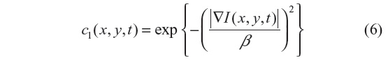
or
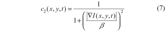
By choosing the first formulation (Equation 6), more emphasis is given to high-contrast edges over low-contrast ones, while the second (Equation 7) focuses on wide regions over smaller ones.10 Both definitions are nonlinear and space-invariant transformations of the initial image. In this study, the diffusion coefficient c2 is used with the different coefficient values β and Δt=1 (hence time is associated with the iteration count).
There are several numerical studies that report the instabilities of the PM method. The main instability observed appears as a “staircasing” effect, where a mild gradient region evolves into piecewise, almost linear segments separated by jumps.10 The following two methods are regularizations of the anisotropic diffusion method, and are possible solutions for these drawbacks.
Improved adaptive nonlinear complex-diffusion despeckling filter
This filter is designed to improve speckle-noise reduction while preserving the edge and image features, and has been applied to optical coherence tomography data.3 The regularization proposed in this scheme includes an adaptive time step Δt and scaling coefficient β. The reason is to have greater sensitivity to the image gradients, since the diffusion coefficient is a function of their magnitude. This results in smaller initial time steps in the diffusion process, and hence emphasis is given to small features of the image during the initial iteration steps.3 The diffusion coefficient used in this method is given by:
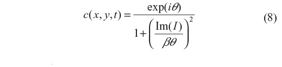
where i=√−1, θ is the phase angle close to zero, and Im(I) stands for the imaginary part of I. One of the main advantages of this formulation is that the diffusion coefficient does not involve derivatives of the image. It has been shown that for small θ, the ratio Im(I):θ is proportional to the Laplace operator I, and hence the diffusion coefficient of Equation 8 can be approximated by:
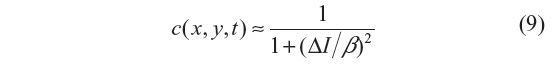
In this work, θ=π/30 is used.3 We note that the diffusion coefficient is approximately a function of the image Laplacian, while for the other filtering methods analyzed, it is a function of the gradient. The locally adaptive β modulates the spread of the diffusion coefficient in the vicinity of its maximum, and hence at edges and homogeneous areas where the image Laplacian vanishes3 and is given by:
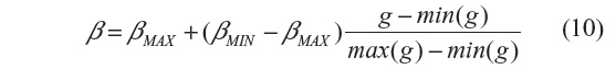
where min(g) and max(g) stand for the minimum and maximum of g, with g = GM,σ * I(n), where * is the convolution operator and GM,σ is the local Gaussian kernel of size n×n pixels, with standard deviation σ and mean 0. Here, n=3, σ=10, βmin=2 and βmax=β.3
A further subtlety is adopted by using a low-pass filtered diffusion coefficient, hence substituting Equation 8 with c’ = GM,σ * c, where the local Gaussian kernel is of size 3×3 pixels and standard deviation σ=0.5. This removes spiky c(x, y, t) points, has proven to be advantageous in increasing speckle removal, and due to the small standard deviation does not change c(x, y, t) noticeably.3
The adaptive time step is given by:
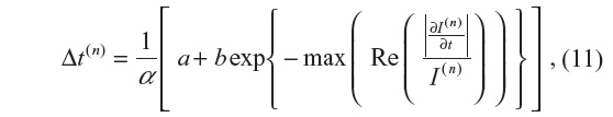
where  is the fraction of change of the image at iteration n, and α, a, and b are constants and control the time step with (a + b ≤ 1). In this work, α=4, a=0.25 and b=0.75, following Bernardes et al.3 The value of β defined in Tables 1 and 2 refers to βmax of Equation 10, while βmin=1.
 | Table 1 Optimal choice of β based on the MSE improvement, as presented in Figure 5, where the number of iterations was fixed to t=30 |
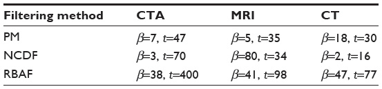 | Table 2 Optimal choice of β and t based on MSE improvement, relative residual error, and SSIM threshold of 0.7, as presented in Figure 6 |
As noted previously, in PM the diffusion coefficient is a decreasing function of the image gradient, which can be regarded as a ramp-preserving process. Considering a ramp function as a model of an edge structure and analyzing further the behavior of the image gradient, we have two main drawbacks. Firstly, the image gradient is not able to detect the ramp’s main features, such as end points. Secondly, the image gradient is uniform across constant ramps, which slows down the diffusion process in uniform regions, and hence is not effective in noise reduction within the ramp edge. These drawbacks are overcome by using the Laplacian as edge detector: it presents high values near end points and low values everywhere else; therefore, it allows for noise reduction over the ramp. One drawback, however, is that noise has large second derivatives and that computation of higher orders will lead to numerical problems for noisier derivative estimates. These issues are overcome with the use of complex diffusion, such that the diffusion process is controlled by the imaginary part of the image signal.
Regularization of backward and forward anisotropic diffusion
Several methods have been proposed for the well-posed nature of the PM method (Equation 4), through appropriate choice of the diffusion coefficients and different regularization approaches. In Guidotti and Longo5 and Guidotti4 (regularization of backward and forward anisotropic diffusion [RBAF]) and references therein, a set of different methods are reviewed and put forward, based on Equation 4.
In Guidotti and Longo5 the work of You and Kaveh11 is followed, where the minimization of a second-order functional is considered. As a result, a fourth-order partial differential equation is considered for the filtering model:
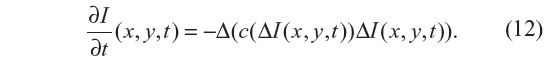
The Laplacian of the image, |ΔI|, is also used here as edge detector instead of the gradient, |▽I|, as in Equation 7 for the PM method. As with the NCDF method, this allows for the preservation of smooth gradients and avoids gradients being sharpened into jumps, in so doing also mitigating the staircasing effect seen in the PM method. Since Equation 12 resembles the behavior of Equation 4, it is also ill posed. Two fourth-order diffusion models based on Equation 12 were proposed in Guidotti and Longo5 where the diffusion coefficient c is either a function of the image gradient or Laplacian. In the present work, c=c(▽I) is adopted.
The regularization approach employed in Guidotti4 relies on the use of fractional derivatives in the edge-detector function within the diffusion coefficient. The resulting equation to be solved is given by:
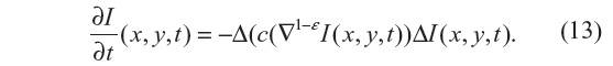
where ε ∈ (0, 1). As a consequence, numerical tests presented in Guidotti4 show a significant reduction of the staircasing effect. Also, considering that |▽1–εI(x, y, t)| is still an edge detector, no blurring effect is observed, unlike those produced by solving the nonlinear anisotropic diffusion in Equation 4, with either diffusion coefficient given by Equation 7 or 8. In this study, Equation 13 is solved with ε=0.2 and Δt=0.02, for which a strong local well-posed nature has been shown in Guidotti and Longo.5
Contrast-enhancement methods
Contrast enhancement of medical images serves to highlight different objects in the scene, so as to improve the visual appearance of an image or to accentuate features to a form that better suits the analysis (eg, feature extraction). Determining a generic and encompassing theory or model for image enhancement is challenging, since defining image quality and standard measures that can serve as design criteria is not straightforward. Here, three popular methods are tested, as seen in Figure 2.
 | Figure 2 Images filtered with PM, NCDF, and RBAF. |
Unsharp masking
The enhanced image IUM(x, y) is computed with two overlapping apertures: one with normal resolution Iorig(x, y), and a correction signal Ihigh(x, y), computed using a linear high-pass filter. The enhanced image is given by:

with λ being the positive scaling constant that controls the level of contrast enhancement achieved at the output image, and was set as λ=0.75, such that the weight of the original image is twice that of the high-frequency spectrum to be added. The correction signal may be simply given by Ihigh = Iorig − Iorig * Gσ, where * denotes convolution and Gσ is a Gaussian function with standard deviation σ and zero mean.12
Histogram equalization
Another means of image enhancement is the modification of the image grayscale histogram under certain criteria, such as forcing the image histogram to be uniform.13 The approach requires first the computation of the transformation function, which is then used to stretch each pixel level to obtain a linear cumulative-distribution function of the image histogram. In this work, an adaptive histogram-equalization technique is employed to emphasize local contrast, such that the image is considered in smaller domains of size n×m, and histograms are generated locally in these domains.14 In the examples seen in Figure 3, we have set n=m=20.
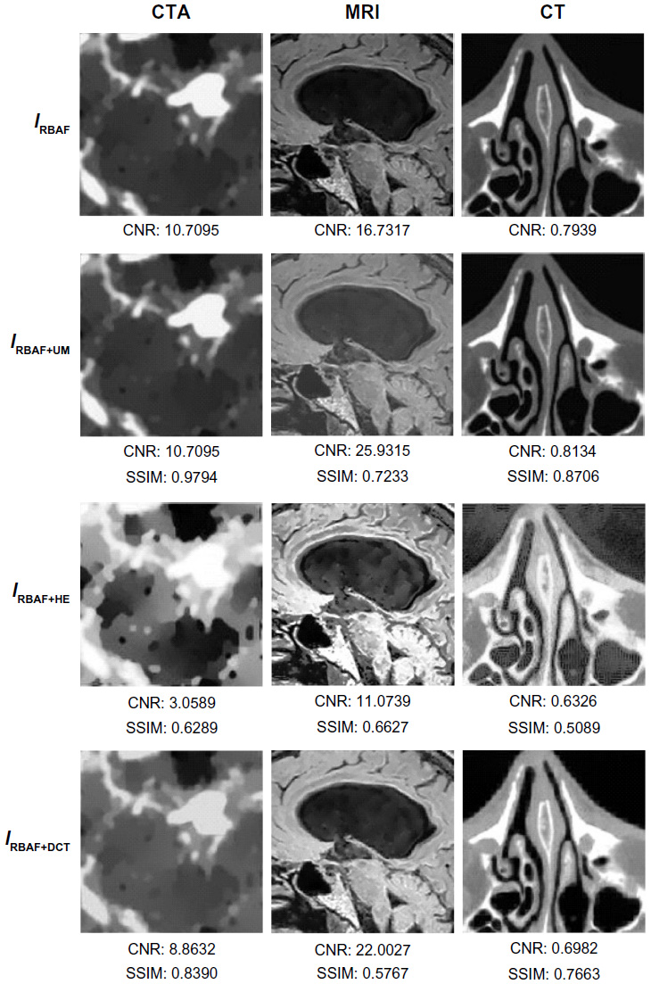 | Figure 3 Images filtered with RBAF and enhanced using UM, HE, and DCT. |
Discrete cosine transform
The DCT technique for contrast enhancement is also performed locally, on nonoverlapping blocks of size n×n. For each block, the DCT is applied and frequencies grouped in three different ranges: low-, mid-, and high-frequency subbands. In order to enhance the image contrast, for each block DCT coefficients are amplified by factor λ, and the enhanced image is subsequently obtained by applying the inverse DCT transform.15 In the present work, n=4. Since higher spatial frequencies are less visible to the human eye, parameter λ is obtained such that higher emphasis is given to these than to lower-frequency subbands.
Segmentation methods
The segmentation of medical images, and thus the location of objects and their boundaries within the image, is an important task in the analysis of the data set. If image segmentation is performed manually, there is inevitably a source of subjective interpretation and subsequently error. Manual segmentation results are often unreproducible, even if performed again by the same individual. An automatic approach is favored, requiring a robust model to differentiate the objects within the images. Such a complex task has led to the development of many mathematical models and numerical methods, of which three main categories are: threshold methods, edge-based methods, and region-based methods. In the present work, one example of each category is employed, respectively: the Otsu method, lines of inflection (zero crossings of second directional derivative), and the watershed method. These simple segmentation methods are widely used, and are still among the most robust and accurate semiautomatic algorithms available. Figure 4 shows resultant segmented images.
 | Figure 4 Segmentations obtained. |
Otsu method
The Otsu algorithm remains one of the most important thresholding methods for image segmentation, due to its simplicity and effectiveness. It is a clustering method, which relies on the histogram of the image grayscale intensities. A constant grayscale intensity-threshold value is chosen to divide the image into two classes. The criterion for defining the threshold is based on minimizing the intraclass variance, or alternatively maximizing the interclass variance, and is accomplished by using solely the zero and first-order cumulative moments of the grayscale histogram.16
Watershed method
In the watershed transformation,17 grayscale images are considered topographic reliefs, which are flooded to resemble lakes by placing a water source at the local minima of each basin. When two lakes merge, a dam is created, and the combination of all created dams define the boundaries of the watershed. Advantages of the watershed transform are that it results in closed-contour object delineation and requires low computation cost in comparison with other segmentation methods. On the other hand, applying a standard morphological transform to the image or its gradient results in an oversegmented image. To overcome this, several methods have been proposed in the literature, including region merging-based methods18 a scale approach19 or methods based on partial differential equations for image denoising and edge sharpness.20 Here, we use marker-based watershed transformations, proposed in Soille.21
Lines of inflection
As discussed for the anisotropic filtering methods, where the diffusion coefficient was spatially modulated, object-edge detection can be identified by maxima of the image-gradient magnitude, or alternatively as the zero crossing of the second directional derivatives. The use of image derivatives for edge detection has been widely used, building upon early work.22,23 The zero crossing of the second directional derivatives for a 1-D signal are the points of inflection in the direction of the steepest ascent. Over a 2-D (or 3-D) image, the zero crossing results in unbroken lines (or surfaces) of inflection.1 The approach requires first computing the image gradient ▽I and the Hessian matrix H, from which the zero-crossing criteria are given by:
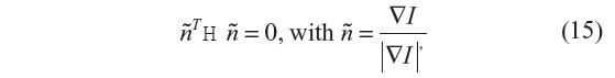
where ñ represents the unit normal vector to the isocontour.
Results
One of the greatest challenges in medical image processing, and especially filtering algorithms, is their sensitivity to optimum parameter selection. In the present work, these include the coefficient β (which appears in the diffusion coefficients) and the stopping criteria T (as the total duration of anisotropic diffusion process). Figure 2 shows the results obtained for each filtering algorithm for an optimal choice of both β and T. It is important to note that the use of the term “optimal” is used here in a loose sense. No formal optimization is in fact carried out. The term “optimal” arises by computing the image metrics discussed for a range of values of the parameters β and T, and subsequently identifying desirable ranges. This procedure is now discussed in greater detail.
In order to select the optimal β, for a given choice of the number of iteration T, we observe the rate of change of the MSE of two images of consecutive incremental β choices. This rate of change is referred to as MSE improvement, and is given by:

In Figure 5, the MSE improvement is shown for the image data sets for a fixed T=30. At the highest value, the optimal choice of β is chosen, and the results are presented in Table 1. In this manner, the problem of identifying optimal choices of β and T is decoupled, and hence an effective choice of β is first identified, and subsequently the selection of the optimal number of iterations, T, for this β value is then required.
 | Figure 5 MSE improvement of each image as β is varied in integer steps from 1 to 50, for T=30 time steps in solving the anisotropic diffusion. |
For a given choice of β, the optimal number of iterations, T, for the filtering process requires use of further image-quality metric criteria. Since the filtering process involves the solution of the anisotropic diffusion equations as a time-marching problem, a possible approach is to halt the filtering when a certain set of metrics fall below a predefined threshold, ε, between two consecutive time steps. In the present work, the relative residual error was the metric chosen for this purpose, specifically |MSEt+1 – MSEt|/|MSEt+1| < ε1, and ε1 =10−2 in combination with a threshold value of SSIM < ε2 and ε2 =0.7, was used throughout. The choice of ε1 is influenced by the need for a small value to identify a convergence of solution, and large enough to make the iterative procedure less computationally demanding. The choice of ε2 is influenced by the importance of allowing the image to evolve and deviate from the original, and yet not to allow too large a distortion that will make the image unrecognizable compared to the original. With this in mind, one can easily compute the ideal β and stopping criteria for any given image. As seen in the left column of Figure 6, the optimal diffusion coefficient is chosen as the maximum MSE improvement between two consecutive β-values is found, and simultaneously the corresponding optimal number of iterations is obtained by |MSEt+1 – MSEt|/|MSEt+1| <10−2 and SSIMβ (t + 1) <0.7. This, depending on the size of each image and respective data set, can be rather computationally expensive; therefore, a parallel implementation was used, which proved to be effective.
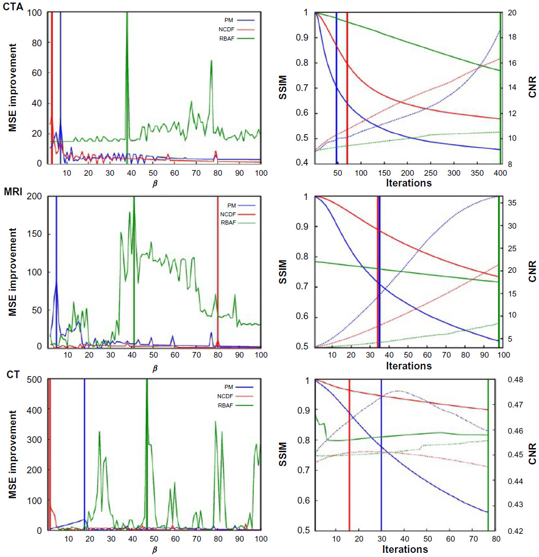 | Figure 6 Use of quality metrics for optimization of β and t for each image, where solid vertical lines indicate optimal choice of these parameters. |
To understand the behavior of each filter as the number of iterations evolves and its relations with SSIM and CNR, results in Figure 6 were analyzed. It is important to recall that the optimal stopping criteria, T, was chosen taking into account simultaneously the relative residual error and the SSIM. We note that the SSIM measure decreases the most for the NCDF and PM filtering methods, indicating that these do not preserve the visual perception of the images well, and the RBAF method outperforms these. On observing the CNR metric, we note that the RBAF method shows little improvement in this regard, while for the NCDF and PM methods the large increase seen is related to the undesirable distortions to the images. Overall, from the results in Figure 6, we conclude that methods that use |▽I| as edge detector (PM and RBAF) are more efficient at preserving edges and important features. Results show that the fourth-order algorithm (RBAF) effectively reduces noise, preserves edges, and important structures, and enhances fine-signal details better than the NCDF and PM methods. The NCDF method is seen to suffer from blurring of object edges to a greater extent than PM or RBAF.
It is interesting to observe the drastic changes seen for both CNR and SSIM when the image is overfiltered. NCDF is specially prone to this, as seen by a major decrease on the CNR after the optimal number of iterations is achieved (see Figure 6, right column). The effects of the image processing can be also appreciated directly as a line plot extracted from the image and the image-gradient magnitude, as shown in Figure 7 for three regions of the magnetic resonance image. The PM and RBAF filtering methods show good preservation of edges and effective removal of noise, while the NCDF method is seen to blur object edges and dislocate their locations slightly. The contrast-enhancement methods UM and DCT are seen to have weak effects on the image and the object boundaries, while the HE approach is seen to overly distort the image and deteriorate it. Figure 3 shows the result of each image (filtered with RBAF) after being enhanced with UM, HE, and DCT. The-contrast enhancement methods are not seen to add effective improvement to the image once anisotropic filtering has been performed.
 | Figure 7 Image-intensity and -gradient magnitude over a line in different regions of the MRI data set. |
Finally, we return to the segmentation methods, results of which are presented in Figure 4. We seek a fully automatic, accurate, and unsupervised method for edge detection. The application of optimized filtering and contrast-enhancement methods prior to segmentation alone cannot guarantee that segmentation results will be anatomically meaningful. The outcome of the segmentation is consequently strongly data-dependent. From the methods proposed, the lines of inflection provide the best results, in that all edges are detected; however, the method does not discriminate the desired objects from the noise or small features.
Conclusion
Medical image processing is a progressive field of research that is increasingly integrated in daily clinical practice. Medical image-acquisition techniques are susceptible to noise, and thus preprocessing images is crucial for the success of any robust and automatic segmentation method.
In this paper, different filtering, contrast-enhancement, and segmentation methods were studied and compared. Together, the steps lead to a complete pipeline whereby medical images are processed to yield a segmentation of relevant objects. Importantly, an approach for automatic selection of filtering parameter choice was developed, proving to be robust and effective. The procedure in identifying the parameter choice automatically relies on firstly identifying a suitable value of β that appears in the diffusion coefficient, and subsequently finding a good value of the total time of filtering – T. The image metrics used to select the suitable parameter values are the MSE and SSIM, more specifically the rate of chance of these metrics and cutoff threshold values.
Overall, results have shown that filtering images with RBAF reduces the uncertainty in object segmentation. No clear advantage was seen in performing contrast-enhancement processing to complement anisotropic image filtering. This is due to the fact that the anisotropic filters rely on edge detection to modulate the diffusion coefficient, and hence explicitly take into account the preservation of edges. As such, an effective anisotropic diffusion filter will include elements of contrast enhancement as an additional beneficial result.
According to the results obtained in this work, we surmise that a robust and attractive pipeline for image processing would involve filtering with RBAF (with the automatic selection of parameters based on image-quality metrics), no contrast enhancement, and segmentation using the zero crossing of the second directional derivative. Further development of the segmentation methods is required, specifically in differentiating the desired features to background objects and remaining pockets of noise. While three different data sets were used, each of a different imaging modality in order to ensure robustness of the methodology and broad scope of the study, it is clearly important to perform additional tests on other patient-specific data sets and indeed verify the general applicability of the pipeline.
Acknowledgments
This work was supported by Fundação para a Ciência e a Tecnologia (FCT) through the grant SFRH/BD/52326/2013 and the Center for Computational and Stochastic Mathematics of the Instituto Superior Técnico, University of Lisbon, in particular the project PHYSIOMATH (EXCL/MAT-NAN/0114/2012). The authors would also like to thank Centro Hospitalar e Universitário de Coimbra for the medical data.
Disclosure
The authors report no conflicts of interest in this work.
References
Gambaruto AM. Processing the image gradient field using a topographic primal sketch approach. Int J Numer Method Biomed Eng. 2015;31:e02706. | |
Perona P, Malik J. Scale-space and edge detection using anisotropic diffusion. IEEE Trans Pattern Anal Mach Intell. 1990;12:629–639. | |
Bernardes R, Maduro C, Serranho P, Araújo A, Barbeiro S, Cunha-Vaz J. Improved adaptive complex diffusion despeckling filter. Opt Express. 2010;18:24048–24059. | |
Guidotti P. A new well-posed nonlinear nonlocal diffusion. Nonlinear Anal Theory Methods Appl. 2010;72:4625–4637. | |
Guidotti P, Longo K. Two enhanced fourth order diffusion models for image denoising. J Math Imaging Vis. 2011;40:188–198. | |
Thibault JB, Sauer KD, Bouman CA, Hsieh J. A three-dimensional statistical approach to improved image quality for multislice helical CT. Med Phys. 2007;34:4526–4544. | |
Flohr TG, Schoepf UJ, Ohnesorge BM. Chasing the heart: new developments for cardiac CT. J Thorac Imaging. 2007;22:4–16. | |
Qi J, Leahy RM. Iterative reconstruction techniques in emission computed tomography. Phys Med Biol. 2006;51:R541–R578. | |
Wang Z, Bovik AC, Sheikh HR, Simoncelli EP. Image quality assessment: from error visibility to structural similarity. IEEE Trans Image Process. 2004;13:600–612. | |
Weickert J. A review of nonlinear diffusion filtering. Scale Space Theory Comput Vis. 1997;1252:1–28. | |
You YL, Kaveh M. Fourth-order partial differential equation for noise removal. IEEE Trans Image Process. 2000;9:1723–1730. | |
Ramponi G. A cubic unsharp masking technique for contrast enhancement. Signal Process. 1998;67:211–222. | |
Hall EL, Kruger RP, Dwyer SJ, Hall DL, McLaren RW, Lodwick GS. A survey of preprocessing and feature extraction techniques for radiographic images. IEEE Trans Comput. 1971;20:1032–1044. | |
Zhu Y, Huang C. An adaptive histogram equalization algorithms on the image gray level mapping. Phys Procedia. 2012;25:601–608. | |
Bhandari AK, Kumar A, Padhy PK. Enhancement of low contrast satellite images using discrete cosine transform and singular value decomposition. Int J Comput Electr Autom Control Inf Eng. 2011;5:707–713. | |
Otsu N. A threshold selection method from gray-leve histograms. IEEE Trans Syst Man Cybern Syst. 1979;9:62–66. | |
Beucher S, Lantuejoul C. Use of watersheds in contour detection. Poster presented at: International Workshop on Image Processing: Real-Time Edge and Motion Detection/Estimation; September 17–21, 1979; Rennes, France. | |
Vincent L, Soille P. Watersheds in digital spaces: an efficient algorithm based on immersion simulations. IEEE Trans Pattern Anal Mach Intell. 1991;13:583–598. | |
Jackway PT. Gradient watersheds in morphological scale-space. IEEE Trans Image Process. 1989;5:913–921. | |
Weickert J. Efficient image segmentation using partial differential equations and morphology. Pattern Recognit. 2001;34:1813–1824. | |
Soille P. Morphological Image Analysis: Principles and Applications. 2nd ed. Heidelberg: Springer; 2004. | |
Haralick RM, Watson LT, Laffey TJ. The topographic primal sketch. Int J Rob Res. 1983;2:50–72. | |
Marr D, Hildreth E. Theory of edge detection. Proc R Soc Lond B Biol Sci. 1980;207:187–217. | |
Bull DR. Communicating Pictures: A Course in Image and Video Coding. Oxford, UK: Elsevier; 2014. | |
Gonzalez RC, Woods RE. Digital Image Processing. 3rd ed. Upper Saddle River (NJ): Prentice Hall; 2008. | |
Jain A. Fundamentals of Digital Image Processing. 3rd ed. Upper Saddle River (NJ): Prentice Hall; 1989. | |
Martini M, Villarini B, Fiorucci F. A reduced-reference perceptual image and video quality metric based on edge preservation. EURASIP J Adv Signal Process. 2012;66–79. | |
Sezgin M, Sankur B. Survey over image thresholding techniques and quantitative performance evaluation. J Electron Imaging. 2004;13:146–168. | |
Weickert J, Scharr H. A scheme for coherence-enhancing diffusion filtering with optimized rotation invariance. J Vis Commun Image Represent. 2002;12:103–108. | |
Zhang X, Feng X, Wang W, Xue W. Edge strength similarity for image quality assessment. IEEE Signal Process Lett. 2013;20:319–322. |
 © 2016 The Author(s). This work is published and licensed by Dove Medical Press Limited. The
full terms of this license are available at https://www.dovepress.com/terms
and incorporate the Creative Commons Attribution
- Non Commercial (unported, 3.0) License.
By accessing the work you hereby accept the Terms. Non-commercial uses of the work are permitted
without any further permission from Dove Medical Press Limited, provided the work is properly
attributed. For permission for commercial use of this work, please see paragraphs 4.2 and 5 of our Terms.
© 2016 The Author(s). This work is published and licensed by Dove Medical Press Limited. The
full terms of this license are available at https://www.dovepress.com/terms
and incorporate the Creative Commons Attribution
- Non Commercial (unported, 3.0) License.
By accessing the work you hereby accept the Terms. Non-commercial uses of the work are permitted
without any further permission from Dove Medical Press Limited, provided the work is properly
attributed. For permission for commercial use of this work, please see paragraphs 4.2 and 5 of our Terms.