Classification of biosensor time series using dynamic time warping: applications in screening cancer cells with characteristic biomarkers

Introduction

Biosensors that produce electrical signals or other time series data present a unique challenge for researchers attempting to use such sensors to classify biological samples. The analysis of such data is complicated by the undesirable variation in the time domain between samples of the same class in addition to variability in the characteristic patterns that may be shared between samples of the same class. In this article, we develop a classification methodology applicable to time series data produced by biosensors. A pseudo-distance metric known as dynamic time warping (DTW) is utilized to quantify the similarity between series in order to construct a classifier. The advantage of this methodology is that it manipulates the time domain of samples in order to better facilitate pattern detection. The use of DTW for quantifying the similarity between time series has been successfully applied in areas such as speech identification^1–3 and medical diagnostics.^4,5 After describing the methodology, we evaluate the performance of such a classifier using simulation studies. Finally, we apply the classification methodology to breast cancer cell detection using a novel single-walled carbon nanotube (CNT) biosensor device.

Methods

The goal of this methodology is to effectively classify time series data for which the class is unknown by utilizing a set of reference time series data for which the class is known. The construction of a similarity-based k-nearest neighbors (k-nn) classifier follows the following steps: 1) a suitable distance metric (or pseudo-metric) for quantifying the dissimilarity between two time series is defined; 2) k-fold cross-validation is used to select classifier’s tuning parameters using training data; and 3) the classifier’s performance is evaluated on an independent set of observations. We represent an individual time series as y = {y_t : t ∊ T}, where T is a time index. We consider T to be a discrete index, which is a valid assumption given that most biosensors sample at some fixed interval. When sample annotation is explicitly shown, y_i,j,t denotes the value of a series from the i th sample of the j th class at time T = t. Since the symbol k is traditionally used to represent an integer in both cross-validation and in nearest neighbors classifiers, we use k to describe the cross-validation parameter and κ to describe the classifier parameter.

Dynamic time warping

The first step we propose in developing the classifier for biosensor data is the identification of a suitable dissimilarity measure. Time series data from familiar biosensor devices such as Electrocardiographs (ECGs) as well as newer devices such as the CNT biosensors are marked by the occurrence of prototypical features that herald the class of the series. Often the time domain of such series is irrelevant and complicates automatic feature detection. As an example, two time series with similar features are shown in Figure 1A. The red series is a phase shift of the blue series with a slight vertical lift. In this situation, a traditional distance metric such as Euclidean distance would conclude that the series are very dissimilar. Yet with respect to the prototypical feature, these series are quite similar. As a result, “warping” of the time domains of one or both of the series (through the insertions of gaps) is necessary for aligning the series for proper quantification of dissimilarity.

Figure 1 Dynamic time warping for time series alignment. Notes: (A) Two qualitatively similar series. Red is a phase shift of blue with a slight vertical lift. Gray dashed line shows the vertical difference. (B) The same series after dynamic time warping alignment.

DTW is a class of dynamic programming algorithms that have been developed in order to align time series in such a manner so that a traditional distance metric can be used to quantify dissimilarity. The resulting alignment of the two series by DTW is shown in Figure 1B.

The utilization of a distance metric on the new warped series, henceforth referred to as a DTW distance, does not satisfy the properties required to be considered as a distance metric. However, DTW distance can still be effectively employed as a dissimilarity measure for constructing classifiers as will be shown later. To calculate the DTW distance between two time series, we utilize the methods presented by Sakoe and Chiba whose original introduction of DTW methodology provides a nice resource for researchers interested in DTW.⁶ Starting with two series, y₁ of length m and y₂ of length n, we first construct an m × n grid of nodes representing a matching of time points from both time indices as illustrated in Figure 2. A warping path,⁷ φ(k) = {(t, t′): k ∊ 1, 2, … K}, through the grid is then sought to minimize the DTW distance, which is defined as:

Figure 2 A grid for computing cumulative cost of alignment.

where d is a traditional distance metric such as the Euclidean metric and w(k) is a positive weight function. The value of the weight function depends on the slope of the line segment joining two points in the grid. Further constraints imposed on the warping path are:

1. Boundary constraints: φ (1) = (1, 1) and φ (K) = (m, n).
2. Step size constraint: φ (k) − φ (k − 1) = {(0, 1), (1, 0), (1, 1)}.

Note that condition 2 does imply that the warping function φ (k) is monotonically increasing. This is important as it avoids loops or other strange warping functions. While there are an infinite number of choices for step weights, in this article we have chosen to explore only two common step patterns that assume that “similar” signals are symmetric. The first choice of weights, Symmetric 1, gives an equal weight for all permissible steps, that is, w(k) = 1∀k. Symmetric 2 weights on the other hand are defined by:

A dynamic programming solution to solving Equation 1 has been previously proposed.⁷ To determine the solution, two matrices Δ ∊ ℝ^m×n and Γ^(m+1)×(n+1) are computed. The first matrix Δ has entries representing the pairwise distances between points in each time series, that is,

where d is a distance metric. The second matrix Γ represents the cumulative cost matrix that determines how the two series should be aligned. To define the second matrix Γ, we begin with stipulating that γ (0,0) = 0, γ (t,0) = ∞, ∀t∊ {1,2, …, m} and γ (0,t´) = ∞, ∀ t′∊ {1,2, …, n}.

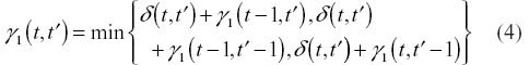
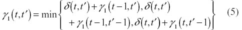
To determine the remaining entries of Γ, we use one of the two following recurrence relations (the first applies to Symmetric 1 and the second to Symmetric 2).

Once Γ has been defined, the reverse of the warping path φ (k) can be found by back-tracing from (m,n) to (1,1). This trace is governed by requiring unit step size either horizontally, vertically, or diagonally – whichever selects the minimal entry in the next step.

k-Nearest neighbors classifiers

With the definition of a pseudo-distance metric (DTW distance) for measuring the dissimilarity of two series, a k-nn classifier is a straightforward choice of classifier.⁸ To build a k-nn classifier, where, k ∊ ℕ, we denote series data as {(y_i, c_i) :i ∊ 1,2, …, N}, where y_i is a time series and c_i = g (g ∊ C denotes the known class of the series). For each observation (y_i, c_i), we find the neighborhood N_κ (y_i) of the κ series y_j with i ≠ j such that these series have minimal DTW(y_i, y_j). We then have empirical estimates of the probability of class membership for (y_i, c_i):

From this set of empirical probability estimates, we chose:

In the case that there are ties between two or more classes, the ties are broken at random. ĉ_i then represents the DTW distance-based k-nn classification of the observation (y_i, c_i). Of course, predicting the class of (y_i, c_i) given that c_i = g is already known is rarely of any interest. Instead, we wish to build a library of series of known class and use this library to predict the class of series for which the class is unknown.

k-Fold cross-validation

A DTW distance-based k-nn classifier has multiple tuning parameters, such as: 1) method of normalizing or preprocessing the series; 2) the choice of weight function in the computation of DTW distances between series; and 3) the choice of k in the k-nn classifier. In order to determine the optimal values of these tuning parameters, we propose using a cross-validation approach.⁸ A training set is first used for k-fold cross-validation tuning parameter selection. While the parameter space for each of the three tuning parameters is infinite, we have restricted the search to values we consider reasonable. In this article, we consider two weight functions previously discussed (Symmetric 1 and Symmetric 2). We consider all integers less than the size of the training set as candidate values of k in the k-nn classifier. Finally, we consider two normalization methods: no normalization and mean–variance normalization such that each series has mean 0 and unit variance. Normalization is one feature of this methodology that warrants further exploration. k-fold cross-validation selection of tuning parameters requires a loss function to quantify the loss of a misclassification. For simplicity, we propose using a 0–1 loss function:

The choice of parameters is sought that minimizes the risk function – the joint expectation of the time series and class membership:

Since no functional form of the right-hand side of Equation 9 is available, it is estimated using cross-validation. Using the notation found by Hastie et al,⁸ we first randomize the training set data into K folds, which can be represented with the mapping κ :{1,2, …, N}→{1,2, …, K}. The k-fold cross-validation risk estimator is then:

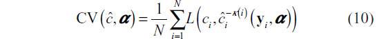
where denotes the classification constructed with the k th fold removed given tuning parameters α. This process is illustrated in Figure 3. Practically,CV (ĉ, α) provides an estimate of the misclassification rate on an independent test set.

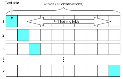Figure 3 A schematic representation of k-fold cross-validation.

Simulation study

In order to evaluate the performance of a DTW distance k-nn classifier, we conducted a simulation study. For this study, we simulated an experiment in which a classifier that can differentiate between two classes of time series is desired, denoted by ξ and η. The simulation study sought to characterize how well such a classifier would perform in an experimental setting. Each class of time series has a different prototypical feature associated with it. To mimic “observed” series from a realistic setting, noise of random length is placed prior to and following the occurrence of the prototypical feature. Additionally, the feature itself is slightly perturbed by random noise. A set of 20 training time series with half belonging to class ξ and half belonging to class η is then used to train a k-nn classifier in which k-fold cross-validation is used to select tuning parameters. Finally, a test set of 20 time series in which the probability of allocation to either class was equal to 0.5 is then used to evaluate the performance of the classifier. The prototype series for class ξ was defined in continuous time as:

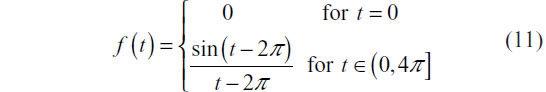
The prototype series for class ξ was defined in continuous time as:

Both prototype series are shown in Figure 4A. Two series y₁ and y₂ with differing values of the scale parameter c perturbing the prototype feature is presented in Figure 4B.

Figure 4 Generation of a prototype feature for each class. Notes: (A) Prototype feature for classes ξ (blue) and η (red). (B) Two series y1 and y2 with differing values of the scale parameter c perturbing the prototype feature.

To simulate observed series rather than prototype signals, “intro” and “outro” random walks are generated, each having random length. More specifically, two integers m₁ and m₂ are drawn with replacement from the sequence {1,2, …, 40}. m₁ and m₂ random walk steps are then generated so that the steps are approximately N(0,1) distributed. The intro and outro random walks are then joined to the prototype feature that has been perturbed using the following equation:

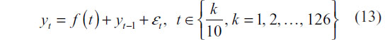
where, with .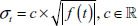

Simulated observed series from each class are shown in Figure 5 alongside the prototype feature for each class. This process for generating the observed series data was used to create the training set consisting of ten series of class η and ten of class ξ. Likewise, the test set was generated consisting of 20 series with the number of series belonging to each class being random with equal class membership probability. A set of training and test series was generated in this manner 10,000 times to simulate 10,000 experiments.

Figure 5 Simulated series from each class. Notes: (A) Three series from class ξ. (B) Three series from class η.

With each simulated experiment, fivefold cross-validation was used on the training set to determine three different tuning parameters. The first tuning parameter considered was the choice of weight function (Symmetric 1 vs Symmetric 2). The second was the choice of k for the k-nn classifier. The final consideration was whether to construct the k-nn DTW distance-based classifier on the raw series or series normalized to have mean 0 and unit variance. The cross-validation used the misclassification rate in order to select optimal tuning parameters. With each experiment, optimal tuning parameter values were found. Subsequently, an independent set of ten series was classified for quantification of error. This set of experiments was conducted for varying values of the scale parameter c. Increasing the value of c decreases the degree of qualitative similarity in the observed prototype feature between series of the same class.

Three scenarios of 10,000 simulated experiments were considered with increasing values of c. A low, medium, and high noise scenario was devised with c values of 0.15, 0.20, and 0.30, respectively. DTW distances were computed using algorithms from the dtw package in R.⁹

Simulation study results

The average cross-validation misclassification rate from the three scenarios of 10,000 simulated experiments is shown in Figure 6. For each scenario, the sample mean and variance of the misclassification rate are given in Table 1.

Figure 6 Training set CV misclassification rate as a function of c. Notes: (A) c = 0.15. (B) c = 0.20. (C) c = 0.30. Abbreviations: CV, cross-validation; k-nn, k-nearest neighbors.

Table 1 Classifier performance during simulation study

On the simulated training folds for each classifier, a 1-nearest neighbor classifier generally showed the lowest cross-validation misclassification rate. Slight dips in the cross-validation misclassification rate are observed at odd numbers, since no tie breaking occurs given an odd number of neighbors. On the simulated test sets, the classifiers performed very well for c values of 0.15 and 0.20. Classifier performance diminished by the value of c = 0.30; however, the prototype feature in these series was fairly well perturbed by noise.

Breast cancer cell detection by EpCAM-CNT biosensors

It is becoming increasingly evident that circulating tumor cells (CTCs) in blood play a vital role in determining the spread of metastatic disease to distant sites. The detection of CTCs and their genetic makeup is therefore highly important for understanding the nature and advancement of the disease. Current technologies such as immunomagnetic methods¹⁰ (Veridex) and CTC chips^11,12 are the primary methods to detect CTCs in blood from patients. While these technologies are impressive, they are not necessarily optimal for rapid identification in clinic. A digital device by which small drops of blood could be rapidly analyzed by microarrays for the detection of CTCs in the clinic would thus have great utility.^13,14 We hypothesized that a CNT device functionalized with an antibody would allow for the rapid detection of CTCs. These devices rely on the principle that each cancer cell possesses thousands of overexpressed particular target receptors, so that cooperative binding to cognate antibodies would yield characteristic spikes in the electrical signal due to free energy change. The reduction in free energy for specific interactions is much higher than nonspecific interactions, and one can use CNT arrays to transduce the change in free energy into electrical signal.¹⁴ From such a CNT array, a characteristic signature indicating specific interactions (CTCs present) versus a characteristic signature indicating only nonspecific interactions (CTCs not present) could be captured. Details of the nanofabrication devices used in this article have been previously discussed by Khosravi et al.¹⁴

To evaluate if devices could differentiate between MCF-7-positive samples and MCF-7-negative samples, both were tested utilizing the nanotube microarrays.¹⁴ Human Buffy Coats were used from Biorepositories at the University of Louisville. The study was approved by the University of Louisville Institutional Review Board (IRB) #10.0428 and the IRB at Worcester Polytechnic Institute IRB #00007374. The negative samples consisted of a buffy coat sample (a layer of centrifuged blood) without the presence of breast cancer cells. The positive samples consisted of a buffy coat sample that was spiked with MCF-7 breast cancer cells. The drain current from the CNT devices was recorded continuously throughout each experiment. The resulting data consisted of time series with characteristic “spikes” occurring after the application of the sample. Two MCF-7 positive and two MCF-7 negative samples are depicted in Figure 7.

Figure 7 Plots of representative electrical signatures from samples used in the construction of a k-nn DTW distance-based classifier for breast cancer surface marker profiling. Notes: (A) Two buffy coat samples. (B) Two spiked buffy coat samples. Abbreviations: k-nn, k-nearest neighbors; DTW, dynamic time warping.

A train–test approach was then used to construct a DTW distance-based k-nn classifier as discussed in. The training data consisted of ten buffy coat samples and 17 spiked buffy coat samples. k-fold cross-validation parameter selection was conducted using tenfold cross-validation on 10,000 bootstrapped samples from the training set of 27 signals for which the class (buffy vs spiked buffy) was known. The tuning parameters selected were those that minimized the mean and variance of the misclassification rate. Once tuning parameters had been selected, 22 test signals (of class unknown to the personnel constructing the classifier) were classified using a DTW distance-based k-nn classifier using the training signals as reference signals. The test set misclassification rate, classifier sensitivity, and classifier specificity were then used as criteria to measure the success of the devices in discriminating between positive and negative samples. Sensitivity is defined as TP/P, where TP represents the number of correctly classified positive (MCF-7 spiked) samples and P represents the total number of positive samples. Similarly, specificity is defined as TN/N, where TN represents the number of correctly classified negative samples (plain buffy) and N represents the total number of negative samples.

Results

A heat map of the DTW signal distances and reference signals used in the k-fold cross-validation tuning parameter selection is shown in Figure 8. In the margins of this figure, a dendrogram of the complete-linkage agglomerative hierarchical clustering⁸ of the same is shown. This demonstrates that on the training data, DTW distance as a dissimilarity measure naturally partitions the sample data into two distinct clusters according to the sample class.

Figure 8 A heat map of training signals. Abbreviation: DTW, dynamic time warping.

Tenfold cross-validation on the bootstrap samples resulted in a final DTW distance-based k-nn classifier utilizing a symmetric two-step pattern and three nearest neighbors. A confusion matrix for the test data is presented in Table 2. The classifier detected the MCF-7 positive samples with 90.9% sensitivity, 81.8% specificity, and a misclassification rate of 13.6%.

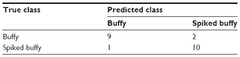Table 2 A confusion matrix for the k-nn DTW-based classifier for detecting breast cancer cells in buffy coat Abbreviations: k-nn, k-nearest neighbors; DTW, dynamic time warping.

Discussion

In this article, we have presented a classification methodology that allows for the discrimination of biological sample types by biosensors that produce electrical signals or other time series data. Such a classifier is well suited for determining the class of series in which there exists a prototypical feature that heralds the class the series belongs to, but the time index is either irrelevant, stretched, or compressed. We have used this methodology to discriminate MCF-7 breast cancer cells present in buffy coat from buffy coat samples without cancer cells by CNT biosensor devices. By demonstrating the ability of a k-nn DTW distance-based classifier to predict the class of the biological sample – whether breast cancer cells are present or not – we have also demonstrated the efficacy of CNT devices for detecting spiked cancer cells in turbid media such as buffy coats. This technique could be useful for screening cancer cells from tissues, liquid biopsy samples, and CTCs in blood in a rapid manner. The handheld and portable nature of the device will be useful for clinical translation.

An important feature of this methodology is extensibility. Many alternative step sizes and alignment constraints have been proposed for the warping path used to minimize the DTW distance.⁶ Additionally, there are an infinite number of choices for the distance metric used in the computation of a DTW distance. While we have chosen Euclidean for its familiarity, other distance metrics may be better suited for specific time series data. Likewise, a k-nn classifier was chosen for simplicity. However, the use of metric multidimensional scaling¹⁵ to map a DTW pseudo-distance matrix constructed from biological time series to a real coordinate space, ℝⁿ, would allow for the use of other classifiers such as linear discriminant analysis or support vector machines.

Acknowledgments

This work was partially supported by the National Cancer Institute through the awards 1R15CA156322 and 7R15CA156322, NSF CMMI 1463869, NSF DMR 1410678, and NSF ECCS 1463987 for B Panchapakesan. Dr SN Rai received support from the Wendell Cherry Chair in Clinical Trial Research and from Dr DM Miller, Director, James Graham Brown Cancer Center, University of Louisville.

Disclosure

The authors report no conflicts of interest in this work.

---

References

1.	Berndt D, Clifford J. Using dynamic time warping to find patterns in time series. In: Fayyad UM, editor. Advances in Knowledge Discovery and Data Mining. Cambridge, MA: AAAI/MIT Press; 1994.
2.	Fu T. A review on time series data mining. Eng Appl Artif Intell. 2011;24:164–181.
3.	Müller M. Information Retrieval for Music and Motion. New York: Springer; 2007.
4.	Alcaraz R, Hornero F, Rieta J. Dynamic time warping applied to estimate atrial fibrillation temporal organization from the surface electrocardiogram. Med Eng Phys. 2013;35:1341–1348.
5.	Tormene P, Giorgino T, Quaglini S, Stefanelli M. Matching incomplete time series with dynamic time warping: an algorithm and an application to post-stroke rehabilitation. Artif Intell Med. 2009;45:11–34.
6.	Sakoe H, Chiba S. Dynamic programming algorithm optimization for spoken word recognition. IEEE Trans Acoust. 1978;26:43–49.
7.	Rabiner L, Juang B. Fundamentals of Speech Recognition. Upper Saddle River, NJ: PTR Prentice-Hall, Inc.; 1993.
8.	Hastie T, Tibshirani R, Friedman JH. The Elements of Statistical Learning. New York: Springer; 2008.
9.	Giorgino T. Computing and visualizing dynamic time warping alignments in R: the DTW package. J Stat Softw. 2009;31:1–24.
10.	Cristofanilli M, Budd GT, Ellis MJ, et al. Circulating tumor cells, disease progression, and survival in metastatic breast cancer. N Engl J Med. 2004;351:781–791.
11.	Nagrath S, Sequist LV, Maheswaran S, et al. Isolation of rare circulating tumour cells in cancer patients by microchip technology. Nature. 2007;450:1235–1239.
12.	Stott SL, Hsu CH, Tsukrov DI, et al. Isolation of circulating tumor cells using a microvortex-generating herringbone-chip. Proc Natl Acad Sci U S A. 2010;107:18392–18397.
13.	Shao N, Wickstrom E, Panchapakesan B. Nanotube-antibody biosensor arrays for the detection of circulating breast cancer cells. Nanotechnology. 2008;19:465101.
14.	Khosravi F, Trainor PJ, Rai SN, Kloecker G, Wicstrom E, Panchapakesan B. Label-free capture of breast cancer cells spiked in buffy coats using carbon nanotube antibody micro-arrays. Nanotechnology. 2016;27:13LT02.
15.	Cox TF, Cox MAA. Multidimensional Scaling. London: Chapman and Hall; 2001.