A New Procedure to Assess When Estimates from the Cumulative Link Model Can Be Interpreted as Differences for Ordinal Scales in Quality of Life Studies

Introduction

Quality of life (QoL) scores from questionnaires are often ordinal variables.¹ Although the ordered categories are often represented by integer values ranging from 1 to a maximum “score”, the difference between any two consecutive categories does not necessarily reflect the same change in perceived well-being. Because of these characteristics, conventional methods for continuous outcomes, such as the linear regression model (LRM), may be inappropriate for analysis of ordinal variables such as QoL measures.^2–4 A number of studies have examined the performance of the LRM in assessing the presence of an association between an exposure and an ordinal score,^2,5–7 but few have investigated its validity in estimating the measure of association as the difference in means of an ordinal score that is used to assess the clinical importance of the effect.^8,9

When analyzing an ordinal QoL score as the outcome of interest in the LRM, there is an implicit assumption that the ordinal score is a good proxy for an underlying (unobserved) continuous QoL level. Thus, the estimated change in the mean of the QoL score per unit change in the exposure variable is being used to infer the change in the underlying unobserved QoL level that is attributable to the exposure, thereby viewing the QoL score as a rounded value of the QoL level. However, there is currently no procedure in LRM analysis that allows the assessment of this proxy assumption, although it is critical to the validity of such inferences. Given the relevance of the difference in mean QoL scores as a measure of clinical importance,^8,9 we propose an alternative to the LRM that assesses the proxy assumption and enables the reporting of the estimates of mean differences when the assumption is adequate.

The cumulative link model (CLM) is a well-established regression model that assumes an ordinal score is an ordered category that arises from the application of thresholds to a latent continuous variable.^10,11 Although the CLM models the cumulative probabilities of discrete ordinal categories,^10,11 a real data application¹² suggested the potential of transforming the CLM estimates to express the effect of an exposure on an ordinal outcome as the difference in the mean score. Specifically, when comparing the effect of an exposure on the ordinal outcome estimated from the LRM and the CLM (with probit link), the authors found that the CLM estimate multiplied by the standard deviation of the ordinal outcome was similar to the LRM estimate. The authors commented that this transformation of the CLM estimate was based on the assumption that the ordinal score was a good proxy for an underlying continuous variable in this example, but did not suggest a formal assessment of this assumption.

In this paper, we propose a new procedure for assessing the proxy assumption with the CLM, and when the assumption is adequate, a valid estimate of the difference in the means of an ordinal score between groups of individuals is obtained from the CLM. This approach allows both statistical and clinical significance to be assessed in a simple two-step workflow that is appropriate for analyzing ordinal scores. We outline the steps when applying our approach, compare the performance of the estimates from the CLM and LRM in simulation studies, and in a real data application investigating the effect of time since diagnosis on fatigue among breast cancer survivors.

Materials and Methods

Applying the Cumulative Link Model (CLM) to Ordinal Scores

Let w denote an ordinal outcome with J categories represented by integer scores: 1, 2, …, J, and let x denote a continuous exposure. The CLM models the cumulative probability of observing each ordinal score with a linear predictor via a link function.^10,11 Specifically, for the CLM with probit link, the probability that an individual with exposure x will have a score w≤j is modelled as follows:

(1)

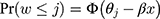
where j= 1,…,J-1, is the cumulative density function of the standard normal distribution, and are category-specific terms. Thus enables the probability of the observed outcome to be expressed in terms of the simple linear function of the exposure in each of the categories, and is referred to as the “link function”. As illustrated in Figure 1, the specification of a negative sign before β in Equation [1] ensures that with β>0, an increase in the exposure (x) increases the probabilities of observing higher ordinal categories, which is in line with the convention of a positive association when the outcome is continuous (as exposure increases the mean increases).¹⁰

Figure 1 An illustration of an exposure effect (β>0) on an ordinal outcome (w) from the cumulative link model with probit link by using the cumulative probabilities associated with the jth category, j=1, …, J-1.

Although the CLM is often introduced as a generalized linear model for ordered categories, it is well known in the literature that the formulation of the CLM with probit link for w can also be based on the following LRM that describes a latent (ie, unobserved) continuous random variable, :^10,11

(2)

where the independent error term, , has a standard normal distribution, ie, 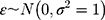. If the  terms in Equation [1] are the thresholds that determine which ordinal score would be assigned for a specific (unobserved) , ie, w=1 when , w=j when for and w=J when , then the β parameter in Equations [1] and [2] is identical^10,11 (see top two rows of Figure 2 for a visual illustration) provided the error term in the LRM has a standard normal distribution. Due to this close connection with the widely used LRM, we focus on the CLM with probit link when developing an estimate for the difference in mean scores from the CLM. Similar to the assessment of model assumptions with residuals from the LRM, recent work¹³ has proposed to assess the assumption regarding the link function of the CLM by using a quantile-quantile plot (qq-plot) of “surrogate residuals”, defined as the difference between a random sample of and its expected value. The surrogate residuals are expected to follow a standard normal distribution if the probit link is appropriate.

Figure 2 An illustration of the relationship between the following three variables when the thresholds (s) are equidistant: the ordinal outcome (w), the latent continuous variable (y*) and the underlying continuous variable (y).

Applying the Linear Regression Model (LRM) to Ordinal Outcomes

The CLM can be used to assess the presence and direction of an exposure effect by modelling the ordered categories of a QoL outcome, and the exposure effect (β) can be interpreted in terms of the cumulative probability of a higher ordinal category for the observed ordinal outcome w.^10,11 After ascertaining the statistical significance of an exposure effect, an important follow-up analysis in QoL studies is to assess the clinical significance of the exposure in terms of some measure of the magnitude of its effect on the continuous QoL that underlies the observed categories. This assessment of clinical significance is often conducted using the LRM of integer scores representing the categories of w, assuming these are good proxies for the underlying QoL levels.

Although the CLM of w in Equation [1] is closely connected with the LRM of in Equation [2], this latent continuous variable does not directly correspond to the underlying QoL level that is proxied by the ordinal scores of w, because the variability of the ordinal scores would clearly depend on the number of distinct values in w, but the error terms for in Equation [2] are restricted to have unit variance so that the exposure effect and thresholds can be identified.¹¹ Hence, we propose a linear transformation of so that the new continuous variable, (where σ>0), spans the range of the ordinal scores and hence represents the underlying QoL level of interest. We refer to y as the underlying continuous variable to differentiate it from the latent continuous variable . Following from the LRM for in Equation [2], the LRM for y is:

(3)

where corresponds to the exposure effect that is approximated by the estimate from the LRM of the ordinal scores, and is interpreted as the difference in the mean ordinal score per unit change in the exposure (x). The new error term, , now has an unrestricted variability σ, and the subscript L in Equation [3] is used to distinguish the parameters in this model from those in the CLM (Equation [2]). The relationship between w, and y is illustrated visually in Figure 2.

Although both and y are unobservable, the exposure effect on (ie, β) can be estimated from the CLM of the observed ordinal outcome w, and given the relationship, , the effect of interest, , can be estimated as . Winship and Mare¹² estimated σ using the standard deviation of the ordinal scores, assuming the proxy assumption is adequate. In the next paragraph, we propose a new procedure to test for the proxy assumption with the CLM that also provides an alternative method for estimating σ when the assumption is found to be adequate.

When the ordinal score representing w is a good proxy (for y), we can view the scores as positive integers derived from rounding-up y when 1.5≤y<J-0.5, and truncating y to 1 and J when y<1.5 and respectively. This is illustrated visually in Figure 2. Equivalently, this relationship between w and y can be described as the categorisation of y with the following thresholds that are one-unit apart: . The proposed linear transformation of to y, ie, , is also applicable to their thresholds; therefore, the consecutive thresholds for (ie, s), are equidistant when the ordinal score representing w is a good proxy for y. Specifically, the successive differences between thresholds, , is constant for , and . We propose to estimate σ from the reciprocal of the slope of a simple LRM of the estimated thresholds (s) from the CLM as the outcome, and the j index as the predictor. Our proposed linear transformation of suggests that is the shift to anchor the first threshold at 1.5 after scaling with σ, and therefore it takes the value (see Section S1 of the Supplementary Material for details). Although there are other thresholds that would make the integer score that represents w a proxy for y (eg, corresponding to the score being a rounded-down integer of y when ), these thresholds will not change , but only result in a shift in .

In summary, the ordinal score representing the ordinal outcome (w) is a good proxy of an underlying continuous variable (y) when the score is approximately a rounded value of y. The CLM assumes that w is generated from applying thresholds (s) to a latent continuous variable (), which we have shown to be a linear transformation of y. Hence, the proxy assumption is valid when the thresholds, s, are equidistant.

Proposed Workflow for Applying the Cumulative Link Model (CLM)

The CLM was developed for modelling ordinal outcomes and is therefore a preferable approach to the widely used LRM for assessing the statistical significance of findings in studies of ordinal QoL scores.¹¹ Our proposed workflow extends the application of CLM to estimate the difference in the mean of an ordinal score per unit difference in an exposure, a statistic often used to assess clinical significance in QoL studies. In Step 1 of the workflow, the presence and direction of the exposure effect are assessed by analyzing the ordinal outcome using the CLM, and the estimate provides a measure of the strength of the exposure effect. When it is desirable to quantify the exposure effect in terms of the difference in the ordinal score, such an estimate can be obtained in Step 2 by estimating the scaling parameter (ie, ) from the estimated thresholds (ie, s) of the CLM to obtain a plug-in estimate, , with standard error , provided the proxy assumption (ie, equidistant thresholds assumption) and the probit link assumption are adequate. The proxy assumption is assessed by comparing two CLMs using the likelihood ratio test, where one of the CLMs has the equidistant constraint on the thresholds (implemented as an option in the ordinal package¹⁴ in R) and the other does not. The appropriateness of the probit link function is assessed by using the surrogate residuals from the CLM (obtained using the sure package^15,16 in R), which follow a standard normal distribution when the probit link assumption is adequate. When there is evidence suggesting the s are not equidistant, the ordinal score may not be a reasonable proxy for an underlying continuous variable, and (from CLM or LRM) no longer has a clear interpretation. In such scenarios, however, the CLM remains valid for making inference on the statistical significance of the exposure effect. The workflow described is summarized visually in Figure 3.

Figure 3 Our proposed analytical workflow for analyzing an ordinal outcome. Abbreviations: CLM, cumulative link model; qq-plot, quantile–quantile plot.

In practice, the minimum value of the ordinal score (denoted by m) is not necessarily 1: for the five subscales of fatigue measured using the Multidimensional Fatigue Inventory (MFI) instrument¹⁷ the minimum score was 4 in our data. Such outcomes can be analyzed by subtracting m-1 from the ordinal score, in which case the estimation of is unaffected, and based on the original observed score can be estimated by adding m-1 to the estimated intercept term.

Simulation Study

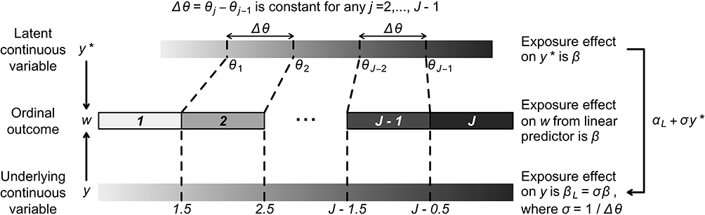
In the simulation study, we generated an ordinal outcome (w) under the CLM framework to assess the performance of the estimate obtained from the CLM using our proposed approach and compared the estimates from our approach with those from the LRM applied to w when the proxy assumption does, and does not, hold. To generate w, we first generated the underlying continuous variable y from Equation [3] where the exposure x was generated from N(1.5,0.5²). To obtain a w that satisfies the proxy assumption, we categorised y into J categories by applying equidistant thresholds: , and represent the categories in using integers . We considered , as 5 or 7 categories is common in practice¹⁸ and J=14 allowed us to assess the impact of a large number of categories on the performance of the two methods. The standard deviation of the normal error distribution took the value , the effect of interest was assigned values of , and the intercept term in Equation [3] was specified as , to ensure no empty categories for w in any of the scenarios considered. An rdinal outcome w with inadequate proxy assumption was generated from y using the following non-equidistant thresholds that ensured all ordinal categories were well represented in all simulation cycles: (i) 1, 2.5, 2.75 and 3.5 for J=5, (ii) 0.8, 1.2, 2.4, 4.4, 5 and 6.6 for J=7, and (iii) 1, 2.7, 4.4, 4.7, 5, 5.6, 6.1, 7, 7.9, 9, 10.1, 11.6 and 13 for J=14 (see visual illustration in Figure S1 in the Supplementary Material).

We assessed the performance of the estimated difference in the mean ordinal score for one-unit change in the continuous exposure x using the CLM with probit link and LRM applied to w, in 2000 simulation cycles. The measures of performance used were the average bias (over the 2000 simulations), the empirical standard error (empirical SE), the average of the model-based standard error (mean SE) and the proportion of simulation cycles where the 95% confidence interval (CI) of included the true value (coverage). The properties of were assessed for different sample sizes (n=300, 1000), number of categories in the ordinal outcome (J=5, 7, 14), different effect sizes ( for zero effect, and 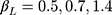for non-zero effect when J=5, 7, 14, respectively) and types of thresholds (equidistant and non-equidistant), creating in total 24 scenarios. We also evaluated the likelihood ratio test of CLM for assessing the equidistant thresholds assumption by using the type I error and power in these simulation scenarios.

Real Data Analysis

We used the CLM and LRM to assess the association between time since diagnosis and fatigue among breast cancer survivors in a survey of 348 women diagnosed with breast cancer at the National University Hospital, Singapore. This study was approved by the National Health Group Domain Specific Review Board (Ref: 2014/00026). Fatigue was assessed using the Multidimensional Fatigue Inventory (MFI) which has five subscales representing General Fatigue, Physical Fatigue, Mental Fatigue, Reduced Activity and Reduced Motivation. Each subscale may take 17 unique values ranging from 4 to 20, with a higher score indicating a greater level of fatigue. The association of interest was adjusted for age, employment status at the time of the survey, ethnicity, cancer stage at diagnosis, type of surgery and the use of chemotherapy. The final dataset included 316 participants who had complete information for all variables of interest.

Analyses were performed using R version 3.6.1.¹⁹ The CLM was implemented using the ordinal package,¹⁴ with surrogate residuals generated using the sure package.^15,16 The LRM was implemented using the lm function.¹⁹

Results

Simulation Study

When the thresholds were equidistant, from the CLM with probit link was unbiased in all the scenarios investigated (see panel A of Figure 4). Although from the LRM was also unbiased when there was no effect of exposure, it was biased for non-zero effect when there were only five categories in the outcome, with the bias decreasing to within ±10% of the true effect when J increased to 14. When the thresholds were non-equidistant, the estimates from both methods were unbiased for zero effect. For non-zero effect, the estimates from the CLM were biased in all scenarios, and similarly, the estimates from the LRM were biased in all scenarios except when J=5. The mean SE of and its corresponding empirical SE were comparable and similar for both methods, and became smaller as expected when the sample size increased in all scenarios.

Figure 4 Mean and standard error (A) and coverage (B) of the estimated difference in mean ordinal scores from the cumulative link model (CLM) with probit link and linear regression model when applied to ordinal outcomes generated with zero and non-zero effects, varying sample sizes (n=300, 1200) and number of categories (J=5, 7, 14). Abbreviation: CLM, cumulative link model. Notes: Solid vertical grey lines indicate the true effect sizes in (A) and the nominal value of the coverage in (B). Dashed vertical grey lines indicate a ±10% deviation from the true non-zero effect in (A) and a ±1% deviation from the nominal value of the coverage in (B). In a scenario with non-zero effect, J=7 and non-equidistant thresholds, the coverage of the linear regression estimate was 48.1% and was beyond the plot range of (B).

When the thresholds were equidistant, the coverage of was generally close to the nominal level of 95% for the CLM with probit link in all the scenarios investigated (see panel B of Figure 4). Although the coverage of for the LRM was generally close to 95% for zero effect in all scenarios, for non-zero effect it was close to 95% only when n=300 and J=14, and decreased with increasing sample size and decreasing number of categories. Since some of the LRM estimates had large bias when there were only five or seven categories, generally a lower coverage was observed for the larger sample size, as the reduced SE of made the 95% CI less likely to cover the true effect. With non-equidistant thresholds, the coverage of from both models was generally close to 95% for zero effect, but lower than 95% for non-zero effect, especially when biased estimates were observed.

When the likelihood ratio test of the CLM was applied to the data generated with equidistant thresholds, the rejection rate was close to the expected level of 5% (range: 4.2%-5.9%) for both zero and non-zero effects (see Table 1). When the data were generated with non-equidistant thresholds, the test had a high power across all scenarios, and detected the non-equidistant thresholds in all of the simulation cycles for both zero and non-zero effects.

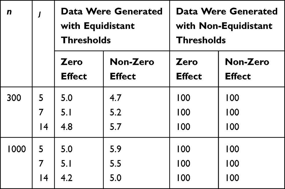Table 1 Percent of Simulation Cycles Where the Likelihood Ratio Test of the Cumulative Link Model for Equidistant Thresholds Assumption Was Rejected, Under Different Sample Size (n), Number of Categories in the Outcome (J) and Exposure Effects

Real Data Analysis

As illustrated in Figure S2 in the Supplementary Material, two of the 17 categories (ie, the 15th and 16th categories that corresponded to scores 18 and 19), were not consistently observed in all five subscales. Hence, we grouped the last three categories (ie, categories 15 to 17) to form a new category and assigned it a score of 18. The numbers of subjects in this new category were 6, 5, 2, 2 and 1 for the General Fatigue, Physical Fatigue, Mental Fatigue, Reduced Activity and Reduced Motivation, respectively. Characteristics of the 316 breast cancer survivors are described in Table S1 in the Supplementary Material. When analyzing the new outcomes with 15 categories, the estimated exposure effect, , suggested that there was a significant negative association between time since diagnosis and the ordinal score for General Fatigue and Mental Fatigue, but the estimated negative associations for the other three subscales were not significant (see Table 2). The qq-plot of surrogate residuals suggested the probit link assumption was adequate for all five subscales (see Figure 5), and the likelihood ratio test suggested no evidence against the equidistant thresholds assumption for all five subscales, except for Mental Fatigue (see Table 2). Thus, the significant (negative) exposure effect on General Fatigue obtained from the CLM can be transformed to the difference in mean scores for further assessment on its clinical importance, resulting in an estimated decrease of 0.154 (95% CI: 0.061, 0.248) in the mean score per year since diagnosis (see Table 2).

Table 2 Estimated Difference in the Mean Scores of the Five Multidimensional Fatigue Inventory Subscales per Year Since Breast Cancer Diagnosis from the Cumulative Link Model (CLM) with Probit Link and the Linear Regression Model (LRM)

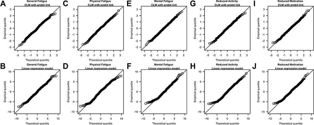Figure 5 qq-plots of surrogate residuals from the cumulative link model (CLM) with probit link (A, C, E, G and I) and residuals from the linear regression model (B, D, F, H and J) when analyzing the five subscales of the Multidimensional Fatigue Inventory. Notes: The last three categories (ie, 15th to 17th categories) of the original subscale scores were grouped into a new category and assigned a score of 18.

Findings from the LRM were consistent with the CLM concerning the direction and statistical significance of the exposure effect on all five subscales. The qq-plot suggested the normal error assumption was generally adequate for all five subscales (see Figure 5). The significant decrease in the mean score for General Fatigue estimated from the LRM (0.139; 95% CI: 0.052, 0.225) was similar to the estimate from the CLM though somewhat lower (percentage difference: 9.7%), and the non-significant decrease in the mean score for Physical Fatigue, Reduced Activity and Reduced Motivation estimated from the LRM and CLM were also similar (percentage difference of 5.7%, 4.1% and 1.6%, respectively). For Mental Fatigue, the difference in the mean score should not be reported as there was evidence against the equidistant thresholds assumption in the CLM analysis.

Discussion

Although modelling the ordered categories of a QoL outcome with CLM will enable one to assess the presence and direction of the effect of an exposure, this alone is not sufficient to enable conclusions of whether the magnitude of the exposure effect is of clinical importance. Investigators often quantify the exposure effect in terms of the difference in the mean QoL score and use this difference to evaluate whether the exposure is of clinical importance. However, such interpretation is valid only when the score is a good proxy for an underlying continuous quantity, which may not hold true in practice. Therefore, there is a need to assess this proxy assumption before reporting the estimated difference in ordinal QoL scores. In this paper, we have proposed a new procedure for assessing the proxy assumption by using the CLM to test for non-equidistant thresholds. When the proxy assumption is adequate (ie, no evidence against equidistant thresholds), the CLM coefficient can be scaled to the familiar measure of association used for assessing the clinical significance of findings (ie, the difference in the mean ordinal score per unit change in an exposure). Using simulated data, we demonstrated the power of our proposed approach in detecting scenarios with invalid proxy assumption and its good performance when the ordinal score was generated under the CLM framework with an adequate proxy assumption. We illustrated the application of the method in assessing both the statistical and clinical significance of an exposure effect in a real-life study of fatigue scores.

An ordinal score is a good proxy for an underlying continuous variable if the score approximates the rounded value of the continuous variable, but this proxy assumption is not assessed in the conventional LRM analyses of ordinal outcomes. The CLM assumes that an ordinal score arises from the application of thresholds to a continuous random variable,^10,11 which allows us to express the proxy assumption in terms of the thresholds by requiring them to be equidistant. When applied to simulated ordinal data, our proposed CLM approach generated unbiased estimates with good coverage only when applied to data generated with equidistant thresholds, and the likelihood ratio test had high power in identifying the scenarios where the equidistant thresholds assumption was inadequate. Although the LRM could perform well in some scenarios when applied to simulated data generated with non-equidistant thresholds, there is currently no way to identify these scenarios in real-life data with the LRM. Hence, our proposed CLM approach is useful and practical for analyzing ordinal data, because it provides a test to assess whether the assumption is met for identifying scenarios where a difference in mean ordinal scores has a valid interpretation.

Our simulation study highlighted the importance of the proxy assumption to ensure only reliable estimates of differences in means are reported. This assumption restricts the differences between consecutive ordinal categories to correspond to the same range of values in the underlying continuous variable, thereby mimicking a characteristic of a continuous quantity where a one-unit change is the same regardless of where it occurs along the continuum. In this way, the difference in means of the underlying continuous variable can be associated with a “scale of measurement” of a one-unit difference in the observed ordinal score. The implication of this assumption is of importance in clinical practice because it allows clinicians to anticipate the amount of change in the exposure associated with a change of one unit in the mean ordinal score, with possible exceptions at the lowest and highest scores. For example, as illustrated in panel A of Figure 6, a change in the underlying continuous variable that corresponds to a -unit change in the exposure results in the same one-unit change in the ordinal score for subjects with initial score of 2 or 5. When the test for equidistant thresholds suggests the proxy assumption is inadequate, this casts doubts on the interpretation of the estimate from the continuous quantity perspective. For example, in panel B of Figure 6, the same amount of change in the underlying continuous quantity resulted in a one-unit increase in the ordinal score among patients with an initial score of 5, but could result in no change or a change of one or two unit(s) in the observed score for patients with an initial score of 2 because of non-equidistant thresholds. Thus, without a formal test of the proxy assumption, there is a danger of drawing conclusions that are not supported by the data. When the proxy assumption is inadequate, the statistical significance of an exposure effect can still be assessed by analyzing the ordered categories using a CLM, but an investigator who also wants to report some measure of clinical significance will need to consider alternatives to the difference in mean scores. For example, in the literature on patient-reported outcomes (PRO) there are toolkits²⁰ developed for conveying clinically relevant information with PRO reference values²¹ and PRO-Bookmarking.²²

Figure 6 An illustration of a one-unit change (indicated by an arrow pointing to the right) along the continuum of the underlying continuous outcome (y) and the corresponding change in the observed ordinal outcome (w) when the thresholds (indicated by vertical ticks) are equidistant (A) and non-equidistant (B). Notes: The relationship between the underlying continuous outcome and the observed ordinal outcome is not applicable to the lowest and highest categories in the ordinal outcome, eg, the first and seventh categories in this example.

In the real data application, the likelihood ratio test suggested adequacy of the proxy assumption for all MFI subscales of fatigue except Mental Fatigue. With 15 categories in the scores, we expected, and observed, the estimated difference in mean fatigue score per year since diagnosis to be similar (less than 10%) between the CLM with probit link and the LRM when the proxy and probit assumptions were adequate. Due to the inadequacy of the proxy assumption, the effect of the exposure on Mental Fatigue should only be reported using the results from Step 1 because the difference in means may not be valid. Our finding of a negative association between fatigue scores and time since diagnosis is consistent with findings in the literature,^23–25 but the estimated reduction (ie, less than 1-unit per year in all five subscales) does not reach the general threshold of a 2-unit difference in MFI subscales for clinical significance.²⁶ Given that the proxy and probit assumptions were found to be adequate for General Fatigue, where a significant decrease in the mean score per year since diagnosis was estimated to be 0.154, breast cancer survivors could expect their General Fatigue score to decrease by 1-unit for every 6.5 (≈1/0.154) additional years since diagnosis.

In this paper, we applied our approach on ordinal QoL outcomes that are constructed from Likert-type variables in a survey by aggregating them to form ordinal categories.²⁷ Although several regression models are available for analyzing such ordinal outcomes,^2,4,11,12,28 they are generally defined and interpreted with respect to the probabilities associated with the ordinal categories (or their related measures) instead of the scores representing these categories. Our proposed transformation of an exposure effect that is based on probabilities to one that is based on mean score leverages on the equivalence between the LRM of a latent continuous variable that underlies the CLM of ordered QoL categories and the LRM of a single continuous variable that underlies the assigned integers to the QoL categories, which is easy to compute from CLM parameters that can be estimated by any standard software package. Alternative approaches for analyzing QoL outcomes are models based on item response theory (eg, the generalized partial credit model^29,30), which have been used in PRO studies.^27,31 Since such models assume the existence of latent traits and express the exposure effect in terms of the probabilities associated with the categories, future work should explore extending our proposed CLM approach to models based on item response theory for analyzing ordinal outcomes.

Although the CLM is robust to misspecification of the link function when assessing the presence and direction of an exposure effect,³² the adequacy of the probit link becomes important when estimating the difference in the means of the ordinal score from the CLM, because it is equivalent to assuming a normal error distribution for the underlying continuous variable of interest.^10,11 Inadequacy of the probit link can be resolved by using other link functions (eg, logit), where our approach can be adapted by considering a different error distribution in Equation [2] that corresponds to the distribution associated with the selected link function¹¹ (eg, logistic distribution). However, regardless of the link function assumed, the proxy assumption still needs to be assessed (via the likelihood ratio test for equidistant thresholds) to ensure valid estimation of the difference in mean ordinal scores. In the simulation studies, the non-equidistant thresholds were detected with 100% power, and generally, we observed an adverse impact on the performance of the CLM and LRM in estimating the difference in mean ordinal scores when the true effect was non-zero. In the supplemental simulation studies, we investigated whether this adverse impact would also be observed when the deviations from equidistance were smaller than the non-equidistant thresholds presented in Figure 4 (see Section S3 of the Supplementary Material). As expected, we observed lower power to detect the smaller deviations from equidistance with a smaller sample size (see Table S3 in the Supplementary Material for additional simulation results). The bias of the CLM in estimating the difference in mean scores decreased as the deviation from equidistance decreased, and the coverage for the smaller deviations from equidistance was close to 95%. For LRM, the bias for the smaller deviations from equidistance were generally comparable to or larger than that presented in Figure 4 and the coverage were comparable to or smaller than that presented in Figure 4, suggesting smaller deviations from equidistance can also adversely impact the performance of LRM. Future work should be conducted to better understand how deviations from equidistance impact the performance of LRM.

When some categories in an ordinal outcome are not observed in the sample (eg, due to small sample size), we can still test for equidistant thresholds with the CLM by combining the ordinal categories. For example, we could group a few categories at the upper or lower extreme if the category that is not observed in the sample occurs at or near the extreme (as in our study of MFI subscales), or group a fixed number of consecutive categories when the category that is not observed occurs among non-extreme values, in order not to distort the potential equidistant thresholds’ structure in the original ordinal outcome. Using the General Fatigue score that had all the categories observed, we performed a sensitivity analysis to assess the impact of collapsing the last three categories in our study and found negligible difference in the estimates obtained from the scores with or without collapsing (see Table S2 in the Supplementary Material for the estimates from the study of the original General Fatigue score).

Conclusion

In conclusion, this paper addresses the dichotomy faced when choosing an ordinal or linear regression model to analyze ordinal outcomes to assess the statistical and clinical significance of an exposure effect on an ordinal QoL score. Using the well-established CLM, we propose a test for the proxy assumption when assessing the clinical significance of an exposure effect in terms of the difference in scores, and a valid estimate for the effect when this assumption is adequate. Although motivated and illustrated in the context of analyzing QoL outcomes, our approach is useful for the study of any ordinal outcomes where interest is focused on estimating the change in the ordinal score per unit change in an exposure.

References

1. Fayers PM, Machin D. Quality of Life: The Assessment, Analysis and Interpretation of Patient-Reported Outcomes.
2. Arostegui I, Nunez-Anton V, Quintana JM. Statistical approaches to analyse patient-reported outcomes as response variables: an application to health-related quality of life. Stat Methods Med Res. 2012;21(2):189–214. doi:10.1177/0962280210379079
3. Alhamzawi R, Ali HTM. Bayesian quantile regression for ordinal longitudinal data. J Appl Stat. 2018;45(5):815–828. doi:10.1080/02664763.2017.1315059
4. Alhamzawi R. Bayesian model selection in ordinal quantile regression. Comput Stat Data Anal. 2016;103:68–78. doi:10.1016/j.csda.2016.04.014
5. Walters SJ, Campbell MJ, Lall R. Design and analysis of trials with quality of life as an outcome: a practical guide. J Biopharm Stat. 2001;11(3):155–176. doi:10.1081/BIP-100107655
6. Walters SJ, Campbell MJ. The use of bootstrap methods for analysing health-related quality of life outcomes (particularly the SF-36). Health Qual Life Outcomes. 2004;2:70. doi:10.1186/1477-7525-2-70
7. Sajobi TT, Zhang Y, Menon BK, et al. Effect size estimates for the ESCAPE trial: proportional odds regression versus other statistical methods. Stroke. 2015;46(7):1800–1805. doi:10.1161/STROKEAHA.115.009328
8. Cappelleri JC, Bushmakin AG. Interpretation of patient-reported outcomes. Stat Methods Med Res. 2014;23(5):460–483. doi:10.1177/0962280213476377
9. Crosby RD, Kolotkin RL, Williams GR. Defining clinically meaningful change in health-related quality of life. J Clin Epidemiol. 2003;56(5):395–407. doi:10.1016/s0895-4356(03)00044-1
10. McCullagh P, Nelder JA. Generalized Linear Models.
11. Agresti A. Analysis of Ordinal Categorical Data.
12. Winship C, Mare R. Regression models with ordinal variables. Am Sociol Rev. 1984;49(4):512–525. doi:10.2307/2095465
13. Liu D, Zhang H. Residuals and diagnostics for ordinal regression models: a surrogate approach. J Am Stat Assoc. 2017. doi:10.1080/01621459.2017.1292915
14. Christensen RHB ordinal—regression models for ordinal data. R package version 2018. 4–19; 2018. Available from: http://www.cran.r-project.org/package=ordinal/.
15. Greenwell B, McCarthy A, Boehmke B sure: surrogate residuals for ordinal and general regression models; 2017. Available from: https://cran.r-project.org/package=sure.
16. Greenwell BM, McCarthy AJ, Boehmke BC, Lie D. Residuals and diagnostics for binary and ordinal regression models: an introduction to the sure package. R J. 2018;10(1):381–394. doi:10.32614/RJ-2018-004
17. Smets EMA, Garssen B, Bonke B, De Haes JCJM. The multidimensional fatigue inventory (MFI) psychometric qualities of an instrument to assess fatigue. J Psychosom Res. 1995;39(3):315–325. doi:10.1016/0022-3999(94)00125-O
18. Krosnick JA, Presser S. Question and Questionnaire Design. In: Handbook of Survey Research. 2nd ed. Emerald Group Publishing Limited; 2010:263–313.
19. R Core Team. R: a language and environment for statistical computing; 2020. Available from: https://cran.r-project.org.
20. Brundage MD, Wu AW, Rivera YM, Snyder CF. Promoting effective use of patient-reported outcomes in clinical practice: themes from a “Methods Tool kit” paper series. J Clin Epidemiol. 2020;122:153–159. doi:10.1016/j.jclinepi.2020.01.022
21. Jensen RE, Bjorner JB. Applying PRO reference values to communicate clinically relevant information at the point-of-care. Medical Care. 2019;57 Suppl 5 Suppl 1:S24–S30. doi:10.1097/MLR.0000000000001113
22. Cook KF, Cella D, Reeve BB. PRO-bookmarking to estimate clinical thresholds for patient-reported symptoms and function. Medical Care. 2019;57 Suppl 5 Suppl 1:S13–S17. doi:10.1097/MLR.0000000000001087
23. Li J, Humphreys K, Eriksson M, et al. Worse quality of life in young and recently diagnosed breast cancer survivors compared with female survivors of other cancers: A cross-sectional study. Int J Cancer. 2016;139(11):2415–2425. doi:10.1002/ijc.30370
24. Klein D, Mercier M, Abeilard E, et al. Long-term quality of life after breast cancer: a French registry-based controlled study. Breast Cancer Res Treat. 2011;129(1):125–134. doi:10.1007/s10549-011-1408-3
25. Hsu T, Ennis M, Hood N, Graham M, Goodwin PJ. Quality of life in long-term breast cancer survivors. J Clin Oncol. 2013;31(28):3540–3548. doi:10.1200/JCO.2012.48.1903
26. Nordin Å, Taft C, Lundgren-Nilsson Å, Dencker A. Minimal important differences for fatigue patient reported outcome measures-a systematic review. BMC Med Res Methodol. 2016;16:62. doi:10.1186/s12874-016-0167-6
27. Fayers PM, Machin D. Quality of Life : The Assessment, Analysis and Interpretation of Patient-Reported Outcomes.
28. Alhamzawi R, Mohammad Ali HT. Bayesian single-index quantile regression for ordinal data. Commun Stat Simul Comput. 2020;49(5):1306–1320. doi:10.1080/03610918.2018.1494283
29. Muraki E. A generalized partial credit model: application of an EM algorithm. Appl Psychol Meas. 1992;16(2):159–176. doi:10.1177/014662169201600206
30. van der Linden WJ, Hambleton RK, eds. Item Response Theory.
31. Nguyen TH, Han HR, Kim MT, Chan KS. An introduction to item response theory for patient-reported outcome measurement. Patient. 2014;7(1):23–35. doi:10.1007/s40271-013-0041-0
32. McCullagh P. Regression models for ordinal data. J R Stat Soc Ser B. 1980;42(2):109–142.
© 2021 The Author(s). This work is published and licensed by Dove Medical Press Limited. The
full terms of this license are available at https://www.dovepress.com/terms
and incorporate the Creative Commons Attribution
- Non Commercial (unported, 3.0) License.
By accessing the work you hereby accept the Terms. Non-commercial uses of the work are permitted
without any further permission from Dove Medical Press Limited, provided the work is properly
attributed. For permission for commercial use of this work, please see paragraphs 4.2 and 5 of our Terms.