Back to Journals » Risk Management and Healthcare Policy » Volume 14
Whether County Lockdown Could Deter the Contagion of COVID-19 in the USA
Authors Chen RM
Received 7 April 2021
Accepted for publication 23 May 2021
Published 23 June 2021 Volume 2021:14 Pages 2665—2673
DOI https://doi.org/10.2147/RMHP.S314750
Checked for plagiarism Yes
Review by Single anonymous peer review
Peer reviewer comments 2
Editor who approved publication: Professor Marco Carotenuto
Ray-Ming Chen
School of Mathematics and Statistics, Baise University, Baise CIty, Guangxi Province, People’s Republic of China
Correspondence: Ray-Ming Chen Email [email protected]
Aim: Whether to lock down a country or not during COVID-19 pandemic becomes a vital issue, since it affects people’s daily life. The objective of this research is to design a measurement that could be utilised to predict the efficacy of a lockdown decision.
Methods: One would expect that the effectiveness of lockdown lies in the assumption that the virus spreads from one area to another area in a rippling way. If the virus spreads in a radiating way, then lockdown should be an effective countermeasure to contain the pandemic. On the other hand, if it spreads indiscernibly or randomly, then a lockdown decision would have lesser or little effect on the containment. We mainly combine graphs and metric to compute correlation matrices, which would measure whether the virus spreads in a rippling way. The metric used is to measure the boundary (or county) distances between counties. We take 3073 counties and equivalents in the USA and explore the property of contagion with respect to distance. The distance between any two counties is measured by the number of neighbours (or counties) between them. Then, we study the relation between contagion and distances. The relation between distance (complexity of neighbouring) and confirmed cases (contagion) is further explored.
Results: Then, we study the relation between contagion and distances. The relation between distance (complexity of neighbouring) and confirmed cases (contagion) could be explored. Our research shows county lockdown in the USA plays no important role in containing the spread of coronavirus for the time being.
Conclusion: Rippling effect in the USA regarding COVID-19 is not significant. This indicates other robust approaches or policies should be taken into consideration, rather than a simple lockdown policy.
Keywords: COVID-19, transport, lockdown, neighbouring, graph, minimal distance
Introduction
Since the COVID-19 pandemic has caused a lot of deaths, tracking the contagion and containing the spread has become an important global issue. The pandemic affects all sorts of people, regardless of their ages.1 The transmissibility and severity of the pandemic have also caused a huge concern about risk management,2 since the strength of the healthcare system would be put into its ultimate test.3 Many countries have adopted preventive measures or containing approaches to combat such pandemic – among them, lockdown probably is the measure taken the most despite its controversy. Lockdown would bring some psychological issues,4 educational problems,5 and so on,6 despite the fact that other alternatives are also adopted.7–9 Decisions of lockdown might affect the trajectory of contagion of COVID-19.12,13 Though some claim they are very effective,14 some regard them controversial.15 Henceforth, some systematic approaches and models are applied in studying the effect of lockdown.10,11 In addition to some criteria for lockdown decision,16 one also needs to consider the timing of lockdown.17 Too early lift of the lockdown might cause a second wave of pandemic, while a delayed one might further deteriorate the economy and normal daily life. In order to evaluate a lockdown decision, one needs to delve into the spreading mechanisms of COVID-19. If it spreads in a pattern that ripples from areas to their neighbouring areas, then one could expect that a lockdown might deter the rippling spread and contain the virus; if not, then one could also anticipate that a lockdown decision would produce little effect on the containment. Such rippling effect is witnessed by studying the spreading behaviours between all the bordering areas. The main objective of this paper is to study the property of such spread in the USA during some period of time.18 We study 3073 Counties and Equivalents in the USA to understand whether lockdown in the county scale is an effective approach for the time being. We devise a systematic mechanism to answer this question by combining the graph theory and metric, in particular the minimal distances between nodes, in one framework. The Counties are identified with nodes (or vertices) of a network (or tree). The number of neighbours from one county to another is associated with the edges. Then a metric of minimal edge is applied to calculate the distance between two counties. This distance will reveal the number of bordered counties between any two counties – the higher the value, the more the bordered counties between the two given counties. The basic idea is if a county has more bordered counties, then it would have higher contacting rate of the virus – if the rippling effect really presents. We will trace the relation between contagion and distance to identify whether the rippling effect really exists in the USA. Henceforth, the values of distances will serve our independent variables. Then we measure the similarity of evolution (from a period of 169 days) between counties via correlation matrix. These values will serve our dependent variable. The relation between distance (complexity of neighbouring) and confirmed cases (contagion) could be explored. Our research shows there is little rippling effect of COVID-19 between neighbouring counties in the USA. This result shall reach a conclusion that a county lockdown decision in the USA plays no important role in containing the spread of coronavirus for the time being. This result also echoes other research of invalidity of lockdown in western European countries.19
Methods
Basic Settings
Let G = (N, E) be an undirected graph, where N is a set of nodes (or vertices) and E is a set of edges. Let n ∈ N be arbitrary. If n = k, then no edge is assumed. Let Ch(p, q) denote all the paths (or chains) connecting nodes p and q in G. Let l1 * l2 denote the concatenation (a new path) of path l1 and path l2. Let |l1| denote the length of the path l1. For a path P, we use Pend to denote its endpoints.
Definition 2.1. (fix neighbours) Let B=k (n) denote the set of all the nodes m, in which there are exactly k edges lying between n and m, ie,
B=k (n) := {m ∈ N: ∃P ∈ Ch(n, m) s.t. |P | = k, Pend = {n, m}}.
Observe that B=0(n) = {n} and B=k+1(n) = 
Definition 2.2. Let B≤k (n) denote the set of all the nodes m, in which there are at most k edges lying between n and m, ie,
B≤k (n) := {m ∈ N: ∃P ∈ Ch(n, m) s.t. |P | ≤ k, Pend = {n, m}}.
Definition 2.3. (minimal nodes with length k) Let  denote the set of all the nodes m, in which there are exactly k edges lying between n and m and there is no path with length less than k that could serve a path between n and m, ie,
  {m ∈ N: ∃P ∈ Ch(n, m) s.t. |P | = k, Pend = {n, m}, Ch(n, m)∩
 ≤k−1(n) = ∅},
where  k−1(n) is the set of all the paths whose initial node is n and whose length is k − 1.
Observe that  , but in general B=k(n) ∩ B=h(n) = ∅ does not hold, if k
  h for all k, h ≤ |l*(n)|.
Definition 2.4. (accumulated minimal nodes with length k) Define

Claim 1. (characterization) For any given n ∈ N, the node set N could be partitioned via the following inductive procedures:
Proof. It follows immediately from the definitions.
Definition 2.5. (chain distance) Let p, q ∈ N be arbitrary. Define δ(q, p) the minimal length of all the paths between p and q, ie, δ(p, q) = min{l: l ∈ Ch(p, q)}.
Claim 2. (distance function) δ is a distance function on G.
Proof. Since no edge is assumed for a node to itself, it suffices to show the triangle property. Let p, q, r ∈ N be arbitrary. Let l1 be a minimal path in Ch(p, q) and l2 be a minimal path in Ch(q, r). Then l1*l2 ∈ Ch(q, r), ie, δ(p, q) + δ(q, r) = |l1| + |l2| ≥ d(p, r).
Example 1. Suppose a geographical structure is shown in Figure 1. Then we could compute some results as listed in Table 1.
 |
Figure 1 A geographical structure: neighbouring. |
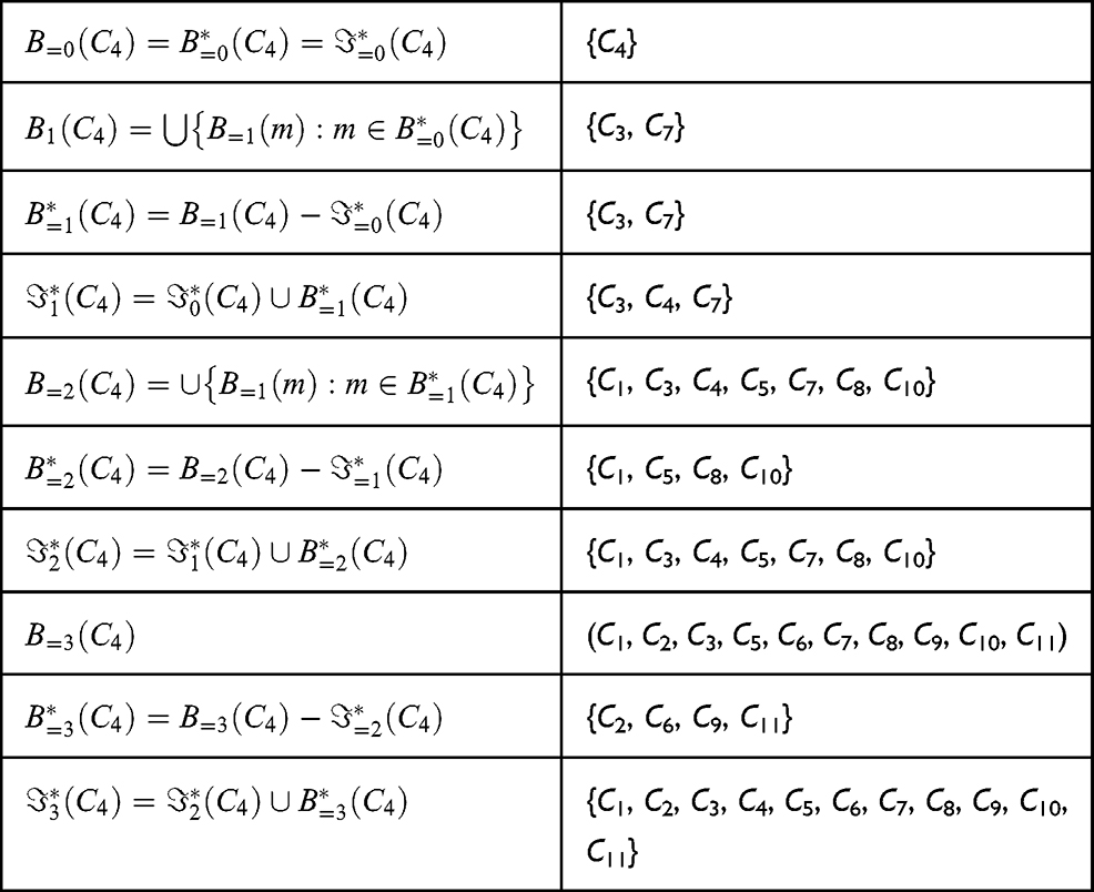 |
Table 1 Comparison for Algorithms Partitioning |
The minimal path might not be unique. As the nodes and the complexity of the geographical structures increase, one needs to devise a systematic approach to compute the values of δ.
Reachability Operators
Let BINk denote the set of all the binary vectors whose length are k. Let


We use the notation  to denote the binary vector
  . Now we devise an algorithm to fast implement Claim 1.
- Label N by N = (n1, n2, · · ·, n|N |) (or simply N = (1, 2, · · ·, |N |)).
- Convert a geographical structure into an adjacency matrix with a cell value 1 if the two nodes are connected directly and 0 if not; the reachability of a node itself is declared to be 0; define
 (or)
(or)  to implement B=1(n).
 where 1 appears in the labelled-n element
 denotes all the nodes corresponding to the values 1 in the vector;
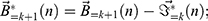
Example 2. This geographical structure could be converted into an adjacency matrix by setting N = {C1, C2, · · ·, C11} and E be specified by the immediate successors as shown in Figure 2.
 |
Figure 2 Adjacency matrix. |
Hence, we have [0]C4 = {C4}, [1]C4 = {C3, C7}, [2]C4 = {C1, C5, C8, C11}, [3]C4 = {C2, C6, C9, C11}.

Though convenient to perform computations based on this, it consumes too much memory and computational resources. We use the first characterization to implement our algorithms. For any vector  , we use
  to denote its jth element. We use
  to denote its Euclidean norm. Let {αj: 1 ≤ j ≤ n} be a set of positive real numbers.
Results
Data Analysis
We use R program 4.0 version to help us implement the procedures in this section.
Procedures
In this section, we list the procedures based on the basic settings in Section 2. These procedures would help us detect whether a rippling effect exists between neighbouring counties in the USA or not.
- After downloading and compiling the files, we use DT for the 3073 counties and their neighbouring Counties and COV ID to read data from the confirmed cases from January 12 until July 8 (or 169 days in total) for the 3073 Counties. The read results are presented in Table 2.
- Then we rename and label the 3073 fips (Counties) by number 1 to 3073. An explicit way of labelling for the confirmed cases could be found in Table 3. Similarly, the renaming of DT., which is implicitly associated in a matrix RDT, is not presented here.
- Based on RDT, we start to calculate the distance matrix DIS, whose size is 3073 by 3073. The calculation of the distance matrices comes directly from Section 2; the resulting distance matrix is presented in Table 4. The values of distance matrix will serve the range of our independent variable.
- Compute the first order and second order of COVID, respectively, to obtain the net increase (decrease). Both are presented in Table 5, where the upper one represents the first order via Matrix SCOVID; the lower one represents the second order via matrix SSCOVID. One observes that the cell value 0.001 indeed is used to replace the original 0 – to avoid the computational problems;
- Based on Table 5, we could compute the correlation matrix for all the counties and the results are presented in Table 6 (or Matrix CORRE); the upper part represents the correlation matrix for SCOVID, and the low one represents the correlation matrix for SSCOVID. These values serve the range of our dependent variables.
- Based on DIS and CORRE, we could plot the graphs as shown in Figure 3.
- Based on the plot, we could decide whether to further apply statistical techniques or not.
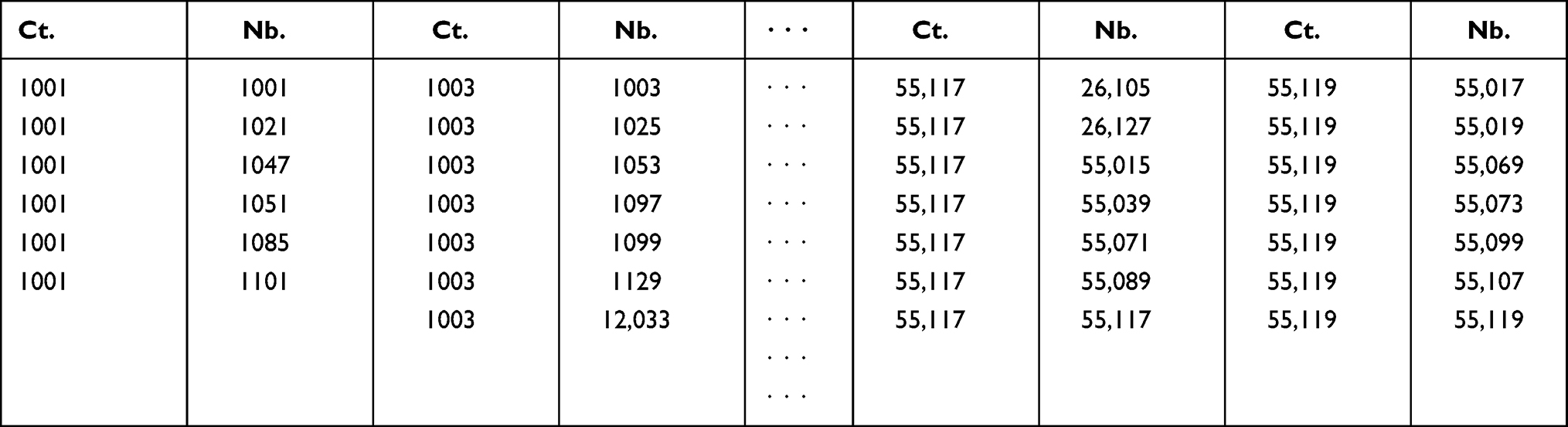 |
Table 2 Raw Data DT: Neighbouring Counties |
 |
Table 3 Raw Data COVID for Confirmed Cases of COVID-19 |
 |
Table 4 Distance Matrix for Counties |
 |
Table 5 First (SCOVID) and Second Order (SSCOVID) for COVID |
 |
Table 6 Correlation for SCOVID and SSCOVID |
Implementation: Preliminary
The downloaded neighbouring information for the counties is presented in Table 2, in which “Ct.” stands for County; “Nb.” stands for Neighbouring Counties; and the cell values are the fips (Federal Information Processing Standards) for the Counties in the USA. In order to facilitate numerical computation, we rename the 3073 Counties names by the number 1 to 3073. The distance matrix is listed in Table 4.
Implementation: Distance Matrix
For the confirmed cases of COVID-19, we extract data from date January 22 to July 8 (169 days in total). The raw data are presented in Table 4.
Implementation: First and Second Order
Here we compute the first order and second order of COVID-19, respectively, to obtain its net increase (decrease). The results are presented in Table 5.
Implementation: Correlation
By Table 5, we compute the correlation matrix for all the Counties as shown in Table 6. We could further visualise the correlations against distances in Figure 3. In this figure, one could easily observe that the physical distance and correlation do not form a recognisable pattern and are very divergent in forming a relation. This also indicates there is no clear rippling effect between the counties.
Conclusion
Lockdown is a controversial global issue. It always has advantages and disadvantages among all sorts of research or policies. The essential part of lockdown or not depends on the effectiveness of such measure – which in turn relies on the rippling spread of the virus. In this article, we sample county data in the USA for a period of time and utilise our minimal metric, which takes the number of bordered counties into consideration, to study the relation between the contagion of COVID-19 and the distances. Our result shows that the spread of virus
 |
Figure 3 SCOVID against Neighbouring Distance. |
Acknowledgments
This work is supported by the Humanities and Social Science Research Planning Fund Project under the Ministry of Education of China (Grant No. 20XJA-GAT001)
Disclosure
The author declares that there are no conflicts of interest regarding the publication of this paper.
References
1. Dong Y, Mo X, Hu Y, et al. Pediatrics. Pediatrics. 2020;145(6):e20200702. doi:10.1542/peds.2020-0702
2. Lipsitch M, Swerdlow DL, Finelli L. Defining the epidemiology of Covid-19-studies needed. New England j Med. 2020;382(13):1194–1196. doi:10.1056/NEJMp2002125
3. Stu¨binger J, Schneider L. Epidemiology of coronavirus COVID- 19: forecasting the future incidence in different countries. Healthcare. 2020;8(2). doi:10.3390/healthcare8020099
4. Webb L. COVID-19 lockdown: a perfect storm for older people’s mental health. J Psychiatr Ment Health Nurs. 2020. doi:10.1111/jpm.12644
5. Sahu P. Closure of universities due to coronavirus disease 2019 (COVID-19): impact on education and mental health of students and academic staff. Cureus. 2020;12:e7541. doi:10.7759/cureus.7541
6. Mukherjee K. COVID-19 and lockdown: insights from Mumbai. Indian J Public Health. 2020;64(Supplement):S168–S171. doi:10.4103/ijph.IJPH_508_20
7. Castaldi S, Romano L, Pariani E, Garbelli C, Biganzoli E. COVID-19: the end of lockdown what next? Acta Biomed. 2020;91(2):236–238. doi:10.23750/abm.v91i2.9605
8. Dzobo M, Chitungo I, Dzinamarira T. COVID-19: a perspective for lifting lockdown in Zimbabwe. Pan Afr Med J. 2020;35(Suppl2):13. doi:10.11604/pamj.2020.35.2.23059
9. Rost G, Bartha FA, Bogya N, et al. Early phase of the COVID-19 out- break in Hungary and post-lockdown scenarios. Viruses. 2020;12(7):E708. doi:10.3390/v12070708
10. Lin Q, Zhao S, Gao D, et al. A conceptual model for the coron- avirus disease 2019 (COVID-19) outbreak in Wuhan, China with individ- ual reaction and governmental action. Int J Infect Dis. 2020;93:211–216. doi:10.1016/j.ijid.2020.02.058
11. Alfano V, Ercolano S. The efficacy of lockdown against COVID- 19: a cross-country panel analysis. Appl Health Econ Health Policy. 2020;18(4):509–517. doi:10.1007/s40258-020-00596-3
12. Roques L, Klein EK, Papa¨ıx J, Sar A, Soubeyrand S. Impact of lockdown on the epidemic dynamics of COVID-19 in France. Front Med (Lausanne). 2020;7:274. doi:10.3389/fmed.2020.00274
13. Nields JA. Alone together in our fear: perspectives from the early days of lockdown due to COVID-19. J Nerv Ment Dis. 2020;208(6):441–442. doi:10.1097/NMD.0000000000001202
14. Sjo¨din H, Wilder-Smith A, Osman S, Farooq Z, Rocklo¨v J. Only strict quarantine measures can curb the coronavirus disease (COVID-19) out- break in Italy, 2020. Euro Surveill. 2020;25(13):2000280. doi:10.2807/1560-7917.ES.2020.25.13.2000280
15. Atalan A. Is the lockdown important to prevent the COVID-9 pandemic? Effects on psychology, environment and economy-perspective. Ann Med Surg (Lond). 2020;56:38–42. doi:10.1016/j.amsu.2020.06.010
16. Claverie JM. A scenario to safely ease the covid-19 lockdown while allowing economic recovery. Un sc´enario de d´econfinement compatible avec une reprise ´economique. Virologie (Montrouge). 2020;24(2):75–77. doi:10.1684/vir.2020.0830
17. Karnon J. A simple decision analysis of a mandatory lockdown re- sponse to the COVID-19 Pandemic. Appl Health Econ Health Policy. 2020;18(3):329–331. doi:10.1007/s40258-020-00581-w
18. USA Covid-19 daily report. Available from: https://usafacts.org/visualizations/coronavirus-covid-19-spread-map/.
19. Thomas A, Meunier J. Full lockdown policies in Western Europe coun- tries have no evident impacts on the COVID-19 epidemic. medRxiv. 2020. doi:10.1101/2020.04.24.20078717,
20. Chen R-M. On COVID-19 country containment metrics: a new approach. J Decision Systems. 2021;1–18. doi:10.1080/12460125.2021.1886625
21. Chen R-M. Quantifying collective intelligence and behaviours of SARS-CoV-2 via environmental resources from virus’ perspectives. Environ Res. 2021;198:111278. doi:10.1016/j.envres.2021.111278
 © 2021 The Author(s). This work is published and licensed by Dove Medical Press Limited. The
full terms of this license are available at https://www.dovepress.com/terms
and incorporate the Creative Commons Attribution
- Non Commercial (unported, 3.0) License.
By accessing the work you hereby accept the Terms. Non-commercial uses of the work are permitted
without any further permission from Dove Medical Press Limited, provided the work is properly
attributed. For permission for commercial use of this work, please see paragraphs 4.2 and 5 of our Terms.
© 2021 The Author(s). This work is published and licensed by Dove Medical Press Limited. The
full terms of this license are available at https://www.dovepress.com/terms
and incorporate the Creative Commons Attribution
- Non Commercial (unported, 3.0) License.
By accessing the work you hereby accept the Terms. Non-commercial uses of the work are permitted
without any further permission from Dove Medical Press Limited, provided the work is properly
attributed. For permission for commercial use of this work, please see paragraphs 4.2 and 5 of our Terms.