Trajectory Modelling Techniques Useful to Epidemiological Research: A Comparative Narrative Review of Approaches

Introduction

In many studies, measured health outcomes are averaged out and their evolution across the entire study sample or pre-specified observed subgroups is analyzed. However, in most cases, unknown or unexpected subgroups of individuals share similar patterns of clinical symptoms, behaviours, or healthcare utilization. Thus, describing populations of individuals using averaged estimates amounts to oversimplifying the complex intra- and inter-individual variability of the real-life clinical context. Trajectory modelling approaches have been developed to address this challenge.^1,2 Individuals can be assigned to homogeneous subgroups (distinct trajectories) that are interpreted as representing similarities on given outcomes.^3,4

Why Modelling Trajectories?

In the case of longitudinal data, a trajectory describes the evolution of a quantity, behaviour, biomarker, or some other repeated measure of interest over time.⁵ To understand the usefulness of trajectory modelling, it is important to define individual-centered statistical approaches. Such approaches focus on the relationships among individuals; their purpose is to classify individuals into distinct subgroups or classes based on personal response patterns.^1,6 Classification is done so that individuals within a given subgroup share greater similarities than individuals from separate subgroups.¹ That said, identifying different subgroups in a given population can be useful in many ways. In fact, grouping individuals according to their similarities and assigning subgroup labels represents a useful option for organizing large datasets and thereby improve efficiency and understanding.^7,8 Researchers can look for subgroups to inform prevention and clinical practice.^7,9 For example, patients may be regrouped according to various trajectories of symptom severity (eg, pain intensity scores over time).^10–12 Once subgroups are identified, trajectory membership can be used as a dependent variable to identify predictors of health trajectories or independent variable to explore their impact on future health outcomes, for example. As shown in Figure 1, trajectory modelling, as compared to measures based on sample means, allows the researcher to better characterize and understand intra- and inter-individual variability and patterns of health outcomes over time. It is useful in exploring heterogeneity of health profiles, to identify vulnerable populations who require better healthcare, and to identify trajectories leading to the best health outcomes. Such approaches can provide scientific evidence to optimize personalized healthcare focused on the needs of specific subpopulations. However, their use is relatively new in the field of epidemiology.¹³

Figure 1 Pain intensity modelling methods: population average models (top) and trajectory modelling approaches (bottom).

To date, few non-technical comparative methodological papers describing trajectory modelling have been published.^9,14 And navigating the literature presents various challenges for non-statisticians. The objective of this review is to provide an overview of the various trajectory modelling techniques and to discuss their applications and differences in order to enable health researchers to choose the technique that best suits their research questions. More specifically, four types of latent class modelling approaches are reviewed: one parametric approach (growth mixture modelling [GMM]), and three semi-parametric approaches (group-based trajectory modelling [GBTM], latent class analysis [LCA], and latent transition analysis [LTA]). The present paper goes beyond previously published reviews,^9,14,15 by comparing those trajectory modelling techniques to other individual-centered statistical approaches such as cluster analysis (nonparametric approach) and sequence analysis (nonparametric approach). This review is written for readers who are not familiar with advanced statistical theory. For each statistical approach reviewed in this paper, we present the basic concepts, the type of data handled, the various steps involved in performing the analysis, the available statistical packages and a real-world example. How best to report the results of trajectory modelling is also covered, followed by a summary of the key points arising from this review.

Trajectory Modelling Techniques

Existing methods and algorithms to examine trajectory patterns or sample subgroups can be categorized into three broad types of approaches: nonparametric, parametric, and semi-parametric.^15–17 Nonparametric approaches make no assumptions about how the data are distributed. Accordingly, the assignment of an individual to a subgroup is based on a dissimilarity measure. In contrast, parametric and semi-parametric approaches assume that data are generated from a finite mixture of distributions. The assignment of an individual to a subgroup is therefore based on conditional probability of that subgroup membership.¹⁸

Latent Class Modelling Approaches

The use of latent variables to model a quantity that is not observed stems from the field of psychology^19–21 and social sciences (developmental trajectories).²² Their use is much more recent in the field of epidemiology.¹³ In pain research, for example, they are increasingly used to model pain severity (eg, intensity scores, interference scores).^{10–12,23-30}

Latent class modelling are statistical models which include random variables that cannot be directly observed.^16,31 Individuals are assigned to latent trajectory subgroups on the basis of their observed symptoms or behaviours.³² Each subgroup is composed of individuals with relatively similar observations/scores on observed behaviours.³³ Latent class modelling approaches can be applied to variables measured in longitudinal or cross-sectional studies.^15,34 They are highly flexible, allowing for a variety of complexities including partially missing data, discretely scaled repeated measures, or time-varying covariates.⁸ In latent class modelling approaches for longitudinal data, at least three measurement time points are required for proper estimation, and four or five measurement time points are preferable in order to estimate more complex models involving trajectories following cubic or quadratic trends.^15,16,22 Rather than evaluating individual time points or change between adjacent time points, longitudinal latent class modelling approaches identify subgroups of subjects who have a similar outcome pattern over the study period as a whole.^1,22

Four latent class approaches are identified in literature. Three are suitable for longitudinal data: growth mixture modeling (GMM),¹⁵ group-based trajectory models (GBTM),²² and latent transition analysis (LTA)³⁵ while one, latent class analysis (LCA), is suitable for cross-sectional data.^34,36 It is common for authors to use inappropriate terms to designate the approach they have used. Thus, non-statistician researchers who would like to use these models in their own research face the difficult task of choosing a suitable approach. In order to shed some light on this issue, an overview of the different latent class approaches and concrete examples of studies reporting the use of theses statistical approaches are presented in Table 1. Each approach is detailed below.

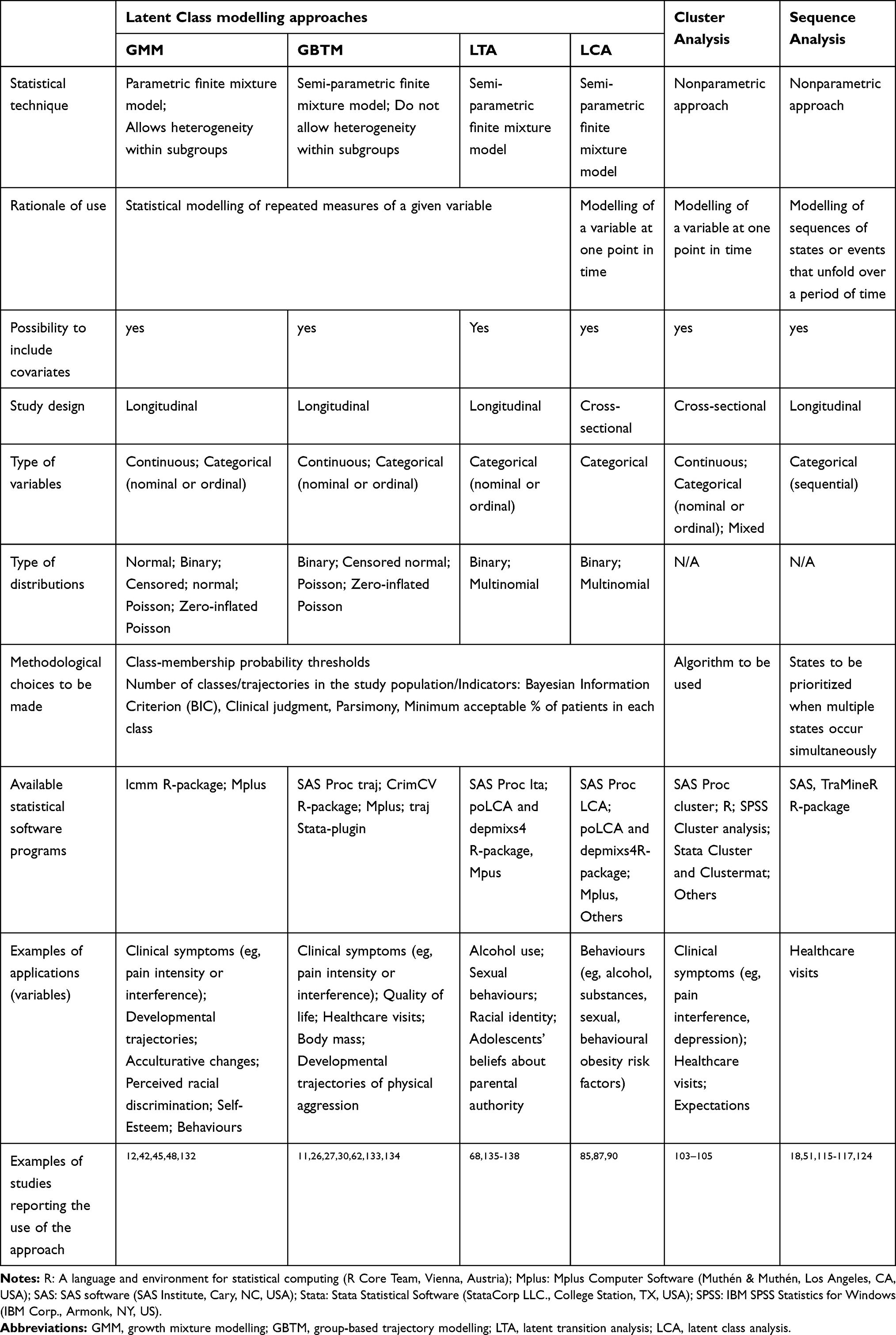Table 1 Overview of the Trajectory Modelling Techniques

Growth Mixture Modelling (GMM)

Presentation

GMM is a finite mixture model. It assumes that in any given population, there exists a finite number of unobserved subpopulations or classes (latent classes) with similar behaviours or experiences. This stands in contrast to classic statistical models which assume that all individuals come from the same population with common population parameters.^1,37 GMM is a parametric model for longitudinal data.³² It estimates an average growth curve for each class and allows for variations between individuals of the same class.^38–40 This heterogeneity within classes is captured by introducing random effects in the model through which variances of the growth parameters can be estimated (intercepts and slopes).^3,41–44 Random effects are thus used to represent the gap between individuals’ latent growth parameters and the population’s mean growth parameter.⁴⁵ For example, in the case of three pain intensity trajectory subgroups (no improvement, gradual improvement, rapid improvement), GMM allows that, in each of these subgroups, any individual can have more intense pain than any other individual of the same subgroup. For each trajectory, GMM estimates an intercept, a slope, as well as a growth parameter variance. Such parameters are estimated by maximizing the log-likelihood function.^37,41 For each individual, the probability of belonging to each class (posterior group probability) is estimated^1,2,41 based on observed data.³ Individuals are then assigned to subgroups based on their higher posterior group probability.^1–3 In GMM, the contribution of covariates (that vary or not over time) can also be modelled.^32,46 Indeed, the probability of belonging to a class may vary depending on covariates, and covariates can influence model coefficients.^{15,16,32,40,41} Once trajectory membership has been established, it can be used as a dependent or independent variable to explore predictors of health trajectories and their contribution to future health outcomes.^{8,13,28,47,48}

Type of Data Handled

The GMM is a model for longitudinal data that has been developed for the study of continuous data.^2,41 However, it was adapted to handle other types of data such as count data (with or without inflation at zero) and categorical data.^1,3,37 For information about sample size calculations specific to GMM, see Muthén and Muthén (2002).⁴⁹

Process

GMM can be implemented using iterative procedures and its implementation requires a priori decisions based on knowledge of the field of research, as well as statistical inference.^1,2,37 To better guide implementation, Ram and Grimm (2009)² have suggested four steps for conducting a GMM analysis:

Step 1: Definition of the Problem and Specification of the Number of Trajectory Subgroups

First, the link between the research area and the method is formalized. Second, an appropriate analysis plan is developed. The expected number of latent classes and the shape of the curve for each class are hypothesized based on the researcher’s knowledge of the field and a descriptive analysis of the raw data. For example, we can expect that patients undergoing surgery will follow various trajectories of postoperative pain intensity (mild versus moderate versus severe pain, followed by an improvement or persistence of pain).

Step 2: Model Specification

During this step, a set of models can be specified and estimated. Researchers may make decisions about growth parameters (intercept, slope variance, and covariance) and the addition of covariates. Substantive theory and previous research should be used to guide these decisions, as much as possible. For instance, if researchers expect three latent classes, they can begin to fit models with two, three and four classes. During these steps, researchers should decide if the shape of each trajectory over time should be linear, quadratic or cubic (intercept and slope parameters). They should also decide if growth factor variances should be specific to each class, if within-class growth factor covariances should be different from zero, and if outcome residual variances should be invariant with respect to class.⁵⁰ Frankfurt et al (2016)⁴⁶ emphasize the importance of properly specifying the model in order to avoid interpretation-based pitfalls. In addition, proper model specification makes the interpretation of GMM results less complex.

Step 3: Model Estimation

GMM can be estimated by maximum likelihood or by Bayesian methods. In this step, researchers should select one of these two estimation methods.

Step 4: Model Selection and Interpretation

The objective of this step is to determine which of the models tested provides the best or most reasonable representation of the observed data. The goodness of fit of the various models should be compared using the Lo-Mendell-Rubin adjusted likelihood ratio test (LMR-LRT, p<0.05 indicates better fit) for nested models (k+1 versus k classes models), and/or the parametric bootstrapped likelihood ratio test (p<0.05 indicates better fit), and/or the Bayesian Information Criteria (BIC) (best models have smaller BIC).⁴⁵ Researchers should also take into account convergence, the ability of the model to provide well separated classes (entropy near 1.0), the proportion of the sample in each trajectory (more than 5% is recommended), average posterior probabilities (near 1.0), parsimony and the usefulness of the observed latent classes in practice.^1,37

Available Packages

GMM can be implemented using Mplus software^1,2,15,37,41 and R through the lcmm package.^51,52 To our knowledge, GMM packages are not available in commercially-available statistical software such as SPSS, SAS, and others.

Advantages and Limitations

As with all other latent class modelling approaches, GMM is useful for accommodating certain technical aspects such as handling missing data, allowing for correlated residuals, and treating residuals in regressions and random effects in mixed effects models as latent variables.^3,53 Unlike other latent class modelling approaches, GMM estimates a mean growth curve for each class and captures individual variation around these growth curves by the estimation of growth factor variances for each class.^1,37 Additionally, because GMM estimates many more parameters than other latent class modelling approaches, the interpretation of results can be complex,⁴⁶ making this approach inaccessible to many health researchers.

Real-World Example of GMM

As a concrete example, Pagé et al (2019)⁵⁴ used such an analytic approach to examine post-operative depression and anxiety trajectories in cardiac surgery patients. Using the Hospital Anxiety and Depression Scale (HADS) scores measured before surgery, at 7 days, and at 3, 6, 12 and 24 months after surgery, a 3-class trajectory solution that included peri-operative covariates was adopted for both anxiety and depression. Trajectory modelling was based on specific selection criteria such as the lowest AIC and BIC, more than 5% of patients in the smallest trajectory subgroup and theoretical soundness. Trajectory memberships were then used as categorical variables in Generalized Estimating Equations (GEE) aiming to examine demographic and clinical characteristics associated with such trajectories. The study led to the discovery of a homogeneous subgroup of patients with unremitted elevated anxiety which predicted the presence of persistent post-surgical pain up to 2 years following the surgery.

Group-Based Trajectory Modelling (GBTM)

Presentation

Like GMM, GBTM—also known as Latent Class Growth Analysis (LCGA)—is a finite mixture model. It is, however, a semi-parametric model for longitudinal data.²² It postulates a discrete distribution of the population and thus makes it possible to distinguish, in the population, subgroups/classes of homogeneous individuals (having a similar trajectory). While GMM estimates the within-class variance,^1,46 GBTM assumes that there is no variation between individuals in the same class (no within-class variance on the growth factors).^3,9,22 Indeed, GBTM is a simplified version of GMM. For example, in the case of the aforementioned three pain intensity trajectory subgroups (no improvement, gradual improvement, rapid improvement), GBTM assumes that in each class, individuals have the same pain intensity evolution. The proportion of the population belonging to each of these subgroups is then estimated. The model also determines, for each individual, the probability of belonging to one subgroup or another (posterior group probability).²² As in GMM, individuals are assigned to a subgroup based on their highest posterior group probability. Parameters are estimated by maximizing likelihood.^22,55–57 Covariates (that vary or not over time) can also be included in the model.⁸

Type of Data Handled

GBTM is a longitudinal data model that was developed for the study of three types of variables: continuous data (particularly psychometric scale data), count data, and categorical data.^8,56 As previously highlighted, it is simpler than GMM. For information about sample size calculations specific to GBTM, see Muthén and Muthén (2002).⁴⁹

Process

Like GMM, the GBTM fitting procedure is iterative and requires prior decisions based on knowledge of the research field.^8,57,58 However, it requires fewer decisions (model specifications) by researchers. Arrandale et al (2006)⁸ suggested four steps for conducting GBTM (similar to GMM steps), which can be summed up as follows:

Step 1: Definition of the Problem and Specification of the Number of Trajectory Subgroups

Same as previously described for GMM.

Step 2: Model Specification

It is suggested to first test a one-group model, then gradually adjust the maximum logical number of subgroups.⁸ This maximum logical number of subgroups should be greater than the expected number of subgroups.² Andruff et al (2009)⁵⁷ suggest that, for datasets with three time points, only a single quadratic shape trajectory model should be tested. If the quadratic component of this model is not significant, the model for a linear trajectory is to be run to determine the BIC value of this model. If the quadratic component of the model for a trajectory is significant, the analysis of the quadratic model for two trajectories is performed. Following these analyzes, the BIC value of the appropriate model with two trajectories will be compared with the BIC value of the appropriate model with one trajectory. This process is repeated with an increasing number of trajectories until the best fit model is obtained, determined by comparing the BIC values.^8,57 Ideally, a combination of knowledge from the field of research and statistical considerations should be used to make a decision about the shape of the trajectory of each subgroup. For example, when modelling the number of healthcare contacts over time, one assumes that patients who have had no contact with the healthcare system throughout the study will belong to a trajectory with 0 order shape (horizontal straight line).

Step 3: Model Estimation

Same as previously described for GMM.

Step 4: Model Selection and Interpretation

Model selection should take into account field knowledge to ensure the usefulness of what is found in practice. It should also consider the following: 1) preference for a useful and parsimonious model that fits the data well; 2) close correspondence between the estimated probability of each subgroup and the proportion of individuals classified in such subgroup according to the rule of attribution of the maximum probability of belonging; 3) average posterior probabilities of subgroup membership greater than or equal to 0.7 for each subgroup; 4) sufficient number of individuals in each subgroup (more than 5%); 5) reasonably narrow confidence intervals; and 6) difference of BICs between two models with different numbers of trajectory subgroups (ΔBIC).^58,59 A set of guidelines are recommended for interpreting ΔBIC.^8,55

Available Packages

The GBTM approach is available in SAS software through the Proc Traj procedure.^8,56 It can also be done with Mplus,^1,37 R through the crimCV package⁶⁰ and the lcmm package,^13,52 and Stata using the traj plugin.⁶¹ GBTM is not available in SPSS or Excel.

Advantages and Limitations

GBTM is a simpler specification of the GMM, and both have the same advantages regarding handling missing data and allowing for correlated residuals. GBTM supposes that all individuals in a trajectory class have the same behaviour, whereas GMM allows for within-class variation.^3,37,40 This means that, when GBTM is used, researchers can discuss differences between subgroups, but not differences within subgroups.⁴⁶ Unlike GMM, GBTM estimates fewer parameters and can thus run faster with fewer errors. Consequently, the results may be easier to interpret because the model is less complex.^1,46,57 For these reasons, GBTM is often the more practical choice for researchers.^9,46

Real-World Example of GBTM

Flint et al (2017)⁶² used a GBTM approach to identify health status trajectories in outpatients with heart failure who participated in a patient-centered disease management intervention randomized controlled trial. Using the Kansas City Cardiomyopathy Questionnaire (KCCQ) measured at baseline, 3, 6 and 12 months, three health status trajectories that included some covariates were identified according to: 1) various statistical indicators (lower BIC and AIC, a significant LMR-LRT and trajectory size more than 5% of the sample), 2) theoretical meaningfulness and conceptual interpretability of the class structure. Trajectory memberships were then used as categorical variable in multinomial logistic regression model to identified predictors of trajectory membership. The study showed that worse depression, symptom burden, and sense of peace were associated with membership in the poor health status trajectory subgroup. Much of the time over one year, the temporal variation of patients’ health status was modest.

Latent Transition Analysis (LTA)

Presentation

LTA is used to analyze changes in multiple categorical variables over time (eg, yes/no, mild/moderate/severe), changes in 2x2, or any contingency tables over time. LTA is a semi-parametric finite mixture model for longitudinal data³⁴ and uses observed data from a set of categorical variables to define a latent variable for each time point.^15,37 The model assumes that individuals can change their class membership over time.⁶³ For example, in the case of three pain intensity subgroups (mild/moderate/severe), LTA allows for individuals to switch from the severe subgroup at one time point to the mild or moderate subgroup at the next time point, and so on. Thus, the primary objective of this approach is to study the probability of transition of an individual from one class at one time point to another class at the next time point.^15,34,37,64 In this model, change is quantified in a matrix of transition probabilities between two consecutive time points.^35,65 The model estimates the following parameters: 1) the latent status membership probabilities at Time 1; 2) the proportion of the population in each latent class at each time point (latent status has been defined as a subgroup/class in which individuals’ memberships can change over time);³⁵ 3) the conditional probabilities of making a transition from one latent status to another over time (eg, probability of being in latent status L2 at Time t given a latent status L1 at Time t-1); and 4) the item-response probabilities conditional on latent status membership (analogous to posterior group probabilities).^35,66,67 At any given time point, a posterior group probability can be predicted.⁶⁷ Hence, individuals can be assigned to a latent class/status at Time 1 using the latent status membership probabilities at Time 1, and at a given time point using the posterior group probabilities.⁶³ Parameters are estimated by maximizing the likelihood function or by the Bayesian method.^35,63,68 Like GMM and GBTM, covariates can be added to LTA models. However, LTA requires that the number of classes be chosen before adding covariates principally to avoid a potential change in class number with and without covariates.⁶³

Type of Data Handled

LTA has been developed to study a set of categorical variables (nominal or ordinal) measured over time.^34,66,69 Furthermore, since the structure of the dataset can lead to large and complex contingency tables when variables have too many categories, it is recommended that they be recoded into as few categories as possible.⁶³ That said, no specific threshold for the number of categories is specified. It is also preferable to use LTA when the number of time points is no larger than 6.⁷⁰ For information about sample size calculations specific to LTA, see Park and Yu (2018) and Wurpts (2012).^71,72

Process

As with GMM and GBTM, implementation of LTA is iterative and requires a priori decisions based on knowledge of the field of research and statistical considerations.^63,73,74 The LTA also requires several steps for its implementation.^63,75

Step 1: Definition of the Problem and Specification of the Number of Trajectory Subgroups

The choice of the number of latent classes is based on the result of a hypothesis test, as well as on the theoretical and specific considerations in the field of research.

Step 2: Model Specification

During this step, researchers make a decision about the time invariance of item-response probabilities, the measurement invariance for transition probabilities (in order to achieve model identification and to facilitate the interpretation of classes prevalence), and the addition of covariates.^67,76

Step 3: Model Estimation

During this step, the estimation method should be chosen before fitting the models. LTA models can be estimated by maximum likelihood using the expectation maximization algorithm.⁶⁷ They can also be estimated with Bayesian methods using Markov chain Monte Carlo algorithms.⁷⁷

Step 4: Model Selection and Interpretation

In the LTA, the AIC and BIC are used to select the best model, favoring the one for which these two values are smaller in absolute value.^69,74

Available Packages

LTA is available in SAS through the Proc LTA,^35,73 Mplus,^37,78 and R through the poLCA⁷⁹ and depmixs4 package.^65,80

Advantages and Limitations

LTA can be very useful to model a change over time and to investigate predictors of this change.³⁵ This model can also be helpful for comparing different subgroups to test for treatment effects and for evaluating the contribution of different measures for each latent status.⁶⁶ However, an important limitation is that LTA requires large sample sizes because of numerous parameters to estimate (eg, transition probability matrix). Indeed, each possible transition may be considered as a separate contingency table. This table often contains a large number of possible response patterns. In fact, many of the cells that have been sampled may be empty. However, the larger the sample size, the lesser the likelihood of sparsity within the contingency table cells.^35,66 Additionally, when the number of time points becomes high (eg, > 6), LTA becomes more complex because of the numerous parameters to estimate.⁷⁰ It should be noted that LTA bears some similarities to Hidden Markov models (HMM). For a more in-depth understanding of such resemblances, see Hickendorff et al (2018),⁸¹ Kaplan (2008),⁸² and Sotres et al (2013).⁶⁷

Real-World Example of LTA

Pat-Horenczyk et al (2016)⁸³ used a LTA approach to assess stability and transitions in post-treatment adaptation profiles of breast-cancer patients. Using a set of indicators of distress and coping strategies measured at baseline, 6, 12 and 24 months postcancer treatment and based on several goodness of fit indicators (lower BIC and AIC, G-square statistic) and interpretability of classes, four post-treatment adaptation profiles were found: distressed, resistant, constructive growth, and struggling growth. A conclusion was that a majority of transitions between adaptation profiles occurred between 6 and 12 months after treatment. Their work was reported as a contribution to the theoretical understanding of the relationship between growth, distress, and coping.

Latent Class Analysis (LCA)

Presentation

LCA postulates that there are underlying unobserved categorical variables that divide a population into mutually exclusive and collectively exhaustive latent classes.⁷⁵ Each latent class represents a subgroup of individuals characterized by a type of response to a set of variables.^34,37,75,84 LCA is a semi-parametric model for categorical cross-sectional data (ie, a non-longitudinal version of LTA).^3,33 In fact, in LTA, LCA is used at each time point to determine classes.³⁴ Hence, like in LTA, the parameters are estimated in LCA by maximizing likelihood or by Bayesian method.^35,69 The contribution of covariates can also be modelled in each class.⁸⁵ Thus, the probability of belonging to a class depends on the values or levels of the covariates.^{35,39,69,85,139}

Type of Data Handled

LCA has been developed for the study of a set of categorical variables measured in a cross-sectional way.^34,69 As with LTA, when variables have too many categories, it is better to recode them into as few categories as possible.⁶³ For information about sample size calculations specific to LCA, see Park and Yu (2018) and Wurpts (2012).^71,72

Process

Steps to perform LCA are the same as its longitudinal version LTA, except for decisions made in model specification regarding the longitudinal aspect in LTA, such as parameter time invariance.^{63,69,73,75,86}

Available Packages

LCA is available in SAS through the Proc LCA.⁶⁹ It can also be done in Mplus,^37,87 R through the poLCA package⁷⁹ and depmixs4 package,^65,80 and in several other softwares less cited in literature.⁸⁸

Advantages and Limitations

LCA is a powerful tool for analyzing the structure of relationships among categorical variables.⁸⁶ It enables researchers to explore and interpret complex contingency tables.⁸⁹ It also provides a method for testing hypotheses regarding the latent structure among categorical variables.³⁶ However, it is only applicable to cross-sectional nominal or ordinal data. LCA is more suitable as an exploratory approach.^34,90 As it analyzes cross-sectional data, LCA cannot really be considered a “trajectory” modelling technique, but the comparison with other latent class approaches was important in the context of the present review.

Real-World Example of LCA

Huh et al (2011)⁸⁵ used a LCA approach to identify distinct subtypes of children with respect to eating, physical activity, and weight perceptions. Using such a set of cross-sectional indicators representing theoretically/clinically relevant dimensions of obesity risk, a 5-class model that included demographic covariates was obtained. Lower BIC and AIC, a significant LMR-LRT, and content and distinctiveness of each class were used. Associations between latent class membership and various variables such as weight, weight perception and sociodemographic characteristics were then assessed. The study showed that children’s weight, ethnicity, sex, and socioeconomic status were associated with latent class membership. In conclusion, the authors suggested that such subtypes of pediatric obesity‐related factors were relevant to the design and implementation of obesity intervention programs.

Further Remarks Regarding Latent Class Modelling Approaches

1. Regarding the use of previous research and theory to guide the number of classes to be modelled, it may be impossible (absence of previous research) or may not be valid in the population under study. In this case, researchers should start modelling iteratively a one class model, then two classes, three classes, etc. (including modelling the number of trajectories they believe to be the right one). Models’ goodness of fit can then be compared.
2. As underlined, latent class models are flexible and can handle missing data when they are missing at random (MAR).^70,91 When missing data are not missing at random (NMAR), authors have even proposed extensions to growth models (like GMM, GBTM and LTA) to take into account this type of missing data.^92–94
3. In addition to the goodness of fit indicators presented earlier, entropy can also be used to evaluate the ability of the model to provide well separated subgroups when using latent class modelling approaches.⁵⁰ In fact, if the goal of the analysis is to classify study participants, which is usually the case with latent class modelling, then it is necessary to report on the performance of this classification.⁹⁵ Entropy summarizes the degree to which the latent classes are distinguishable and the precision with which individuals can be assigned to classes. It is a function of the individual estimated posterior probabilities and ranges from 0 to 1 with higher values indicating better class separation. However, there are no cut-off criteria for interpretation.¹ In addition, the entropy can be overestimated in the case of the addition of covariates to the latent class model (one-step-model), which inflates confidence in the classification.⁹⁵
4. It is important to know that for GMM, GBTM, LCA and LTA, the underlying trajectories are not observed and will never be known. Hence, when reporting and interpreting results, they should not be described as such. In addition, derived trajectories should only be interpreted in the context of the population they were studied in and they might not be valid in different populations.
5. Once trajectories (classes/subgroups) are determined, there are different methods to associate these trajectories with precursors or later outcomes. It should be noticed that methods used to assess such associations can produce very different results.^14,96,97
6. Latent class modelling approaches are useful to answer many types of research question. However, researchers should be aware it is always possible that the best model is a one-class model, that the results of goodness of fit of the modelling are poor, or that the results are not interpretable. In these cases, researchers can use common modelling approaches such as regression models or nonparametric modelling approaches such as those covered in the next sections.

Other Modelling Approaches

Cluster Analysis

In some situations, latent class modelling approaches are not suitable due to the nature of the data. In these instances cluster analysis can be used as a nonparametric alternative to the LCA approach (eg, when assumptions are not met or if variables of interest are not categorical).

Presentation

In the field of data mining, the term “cluster” refers to a subgroup of objects that are similar.⁹⁸ Cluster analysis is a fully nonparametric approach for cross-sectional data, aiming to classify similar objects or individuals into discrete classes, the objective being to determine the number and the composition of classes.^7,74,98,99 The similarity between individuals is measured using a distance measure.^7,100 The objective of this approach is to maximize intra-group similarity while minimizing inter-group similarity.⁹⁸

In cluster analysis, various methods can be used to classify data:^7,98,101 1) Partitioning method: Builds several partitions then evaluates them according to certain criteria (eg, k-means, k-medoids). The number of clusters (k) must be determined in advance; 2) Hierarchical methods: Creates a hierarchical decomposition of objects according to certain criteria. This approach uses the distance matrix as a grouping criterion. The cluster number (k) does not need to be predefined; a stop condition must, however, be specified (eg, the number of common neighbours of two clusters); 3) Density-based methods: These are based on notions of connectivity and density. Clusters are seen as dense regions separated by regions that are less dense; 4) Grid methods: These are based on a multi-level structure of granularity. Each of these methods uses a distance measure that should be chosen depending on the type of data.^100,102 Classical measures of distance include Euclidean distance, Manhattan distance, and correlation-based distances (Pearson correlation distance, Eisen cosine correlation distance, Spearman correlation distance, and Kendall correlation distance).

In cluster analysis, each individual or object belongs to a single cluster, and the complete set of clusters contains all individuals.⁷ Cluster analysis is frequently used in epidemiology and public health,^103–106 as well as in psychology and social sciences.^107–109

Type of Data Handled

Cluster analysis can support cross-sectional data of various types, namely continuous data, categorical data (ordinal or nominal), and mixed data.^7,98,101 Amatya et al (2013) provide information about sample size calculation.¹¹⁰

Process

The steps for building clusters depend on the chosen method and distance measure.^7,98,101,111 However, three main steps stand out in literature:

Step 1: Data Exploration

Given that the choice of distance measure depends on the type of data used, an exploratory analysis of the database is necessary to get an idea of the data type and distribution. In some cases and depending on what is sought, the data can be transformed (eg, a continuous variable may be recoded into a binary variable).

Step 2: Method and Distance Measure Selection

Once the nature of the data is known, the distance measure and the cluster analysis method can be chosen. However, different methods can produce very different results using the same set of variables. Cluster analysis methods are highly dependent on the distance measure chosen. The definitions of distance vary depending on the nature of the variables (continuous, categorical, or mixed data). Sivarathri and Govardhan⁹⁸ summarized the various distance measures according to the type of data used. In addition, Everitt et al⁷ suggest distance measures be used in specific cases as follows: 1) Continuous data: Minkowski distance; 2) Binary data (categorical data with two categories): based on the contingency tables, simple matching coefficient if the objects are symmetrical, or Jaccard coefficient if the objects are asymmetrical; 3) Categorical data (>2 categories): simple matching coefficient according to the total number of variables and the number of matches, or create a binary variable for each modality and use the approach for binary data; 4) Mixed data: Combination of two or more of the aforementioned distance measures. The quality of the classification will depend on the chosen distance measure and method.^7,74,98,101

Step 3: Method Implementation and Result Interpretation

Cluster analysis is conducted according to the specificities of the selected method and distance measure. The distance measure is used to find the degree of similarity between two objects and to decide which grouping to perform. The results of the distance measurement between two objects range between 0 and 1, where “0” means that the objects are dissimilar, and “1” means that they are completely similar.

Available Packages

Cluster analysis can be conducted in several common software packages such as the SAS proc cluster, a combination of packages under R, cluster and clustermat commands under Stata, cluster syntax under SPSS, and many other applications or softwares rarely cited in literature.^7,98,101,111

Advantages and Limitations

Cluster analysis is useful in the exploration of cross-sectional multivariate data. By organizing such data into subgroups or clusters, this approach may help researchers discover the characteristics of potential structures or patterns.⁷ However, cluster analysis does not provide a detailed perspective on individual differences within subgroups. In contrast, latent class modelling is more flexible than cluster analysis for identifying heterogeneous subgroup populations.^1,16 Like LCA, cluster analysis analyzes cross-sectional data and cannot really be considered a “trajectory” modelling technique.

Real-World Example of Cluster Analysis

In order to study common mechanisms and underlying genetic factors responsible for spontaneous preterm birth, Esplin et al (2015)¹⁰⁴ used a hierarchical cluster analysis to identify homogeneous phenotypic profiles. Using cross-sectional clinical and demographic variables, binary indicators for each phenotype, weighted score for each phenotype category, and a dissimilarity matrix, a 5-clusters solution was found. According to the hypothesis that cluster analysis using subcategories within phenotypes might identify subsets of women with a similar genetic risk for spontaneous preterm birth. One of the phenotypic clusters was then selected for candidate gene association.

Sequence Analysis

When researchers are interested in grouping individuals showing similar sequences of events over time, sequence analysis is of great relevance. For example, in the field of health service research an individual’s care trajectory could be conceptualized as a pattern of healthcare events, considering variables related to the patient, illness condition, care providers, care settings, treatments, and time.¹¹²

Presentation

Sequence analysis, is a fully nonparametric method for longitudinal sequential data which aims to classify sequences of observations according to their similarity³³ (care trajectory example: emergency department visit - hospitalization - home - general practitioner visit). This approach was originally developed for the analysis of protein and DNA sequences.¹¹³ However, it has been applied in many other contexts since then, including in epidemiology and public health,^114–118 as well as in psychology and social sciences.^{4,51,119–122} First, sequence analysis computes the matrix of dissimilarities or distances between individuals. These dissimilarity matrices are then used by classification approaches—mainly cluster analysis methods—to determine subgroups or classes of observations according to their similarity.^18,123 Based on a previous “multidimensional model of care trajectories”,¹¹² a comprehensive approach of sequence analysis, considering simultaneously illness condition, care providers and care settings, has recently been proposed.¹²⁴ As in other classification methods presented in this review, subgroup membership can be used as a dependent or independent variable to explore predictors of health trajectories and their contribution to future outcomes.

Type of Data Handled

Sequence analysis can handle categorical longitudinal data (presence of an event, yes/no) to describe the sequences of events.^125,126 More information about sample size calculation can be found in literature.^127,128

Process

The modelling of trajectories using a sequence analysis approach requires several analytic steps:

Step 1: Data Exploration and Preparation

A state sequence data must be created from the raw data for analysis. For example, make sure to choose a suitable alphabet for each state (eg, H for hospitalization, E for Emergency visit, etc).^18,123 The sequences of states must be positioned on a time axis, with the time period (daily, weekly, monthly, annual, etc.) clearly defined. For each time period, a single state must be chosen by the researcher.¹¹⁴ This step is relatively complex, as there are many possibilities for determining the state to prioritize cases where there are more than one state to choose from at a given time point⁴ (for example, in the case of monthly healthcare utilization, an individual could have one hospitalization and one emergency visit in the same month).

Step 2: Distance Measure Selection

At this step, researchers should choose an appropriate distance measure: update-based distances or distances based on subsequences. Update-based distances measure the distance between two sequences by counting the minimum number of update operations required to transform one sequence into a perfect copy of the other.¹²⁵ These distance measures (and their many variants) are called “optimal matching”. Thus, the distance between two trajectories is a function of the costs (in terms of running time and computer memory space) attributed to operations such as insertion, deletion and substitution.^4,18,125,129 The identification of the relative cost of all operations is essential to determine the distance between sequences. These require an a priori definition by the researcher.^4,126 In contrast, the distances based on the subsequences assess the distance between the sequences by counting the number of common subsequences.^4,18 Optimal matching is, however, the most widely used distance measure in literature. Studer and Ritschard¹¹⁹ provide guidelines on choosing the right distance measure.

Step 3: Sequence Analysis and Interpretation of Results

The calculation of the distances between all the sequences gives a matrix of distance. Sequence analysis uses this distance matrix to partition sequences into more or less homogeneous subgroups. Various methods of cluster analysis are suitable for this purpose, including hierarchical methods.^18,125

Available Packages

Sequence analysis can be performed via several software packages such as SAS, Stata, SPSS, R, and many others seldom cited in literature. However, to date, the most powerful and complete way to perform sequence analysis is the TraMineR package of the R software.^121,125,129

Advantages and Limitations

The advantage of sequence analysis lies in the fact that, when researchers are interested in the order of the occurrence of events over time, this approach enables the grouping of individuals by classes based on the similarity of their path. However, if researchers are interested in the number of events over time, sequence analysis is less appropriate. Regarding management of missing data in sequence analysis, Gabadinho et al (2011)¹²⁵ and Halpin (2016)¹³⁰ have suggested many approaches such as multiple imputation for categorical data and taking into account the position of the missing value on the time axis (left, in-between and right missing values). However, as Ritschard and Studer (2018)¹²³ highlighted, this issue have no definitive solution and deserve further research.

Real-World Example of Sequence Analysis

Vanasse et al (2020)¹²⁴ used sequence analysis to identify similar care trajectories among patients after a first hospitalization for chronic obstructive pulmonary disease (COPD). The care trajectories consisted of sequences of healthcare utilization over a one-year period, with “weeks” as the time unit. Using the information about medical visits and hospitalizations from Quebec’s medico-administrative data, and based on several tools and specific selection criteria (optimal matching, pooled distance matrix, Ward’s linkage criteria and sum of squares or inertia), five subgroups were found resulting in a new care trajectory typology. Afterwards, patients’ characteristics were compared across care trajectories subgroups. The study revealed that patients in the 3rd highest utilization care trajectory subgroup were older, had more comorbidities and a more severe condition at the index hospitalization.

How to Report Trajectory Modelling Methods

When reporting individual-centered statistical approaches in scientific papers, researchers should make sure that the analyses are described in sufficient detail so other researchers are able to reproduce them.¹³¹ Hence, scientific papers should contain: 1) data presentation (identify dependent variables and possible covariates, and mention all data treatment [eg, creating new variables, recoding certain variables to facilitate analysis, etc.]); 2) the trajectory modelling technique and a justification for its use; 3) specifications regarding the logic and criteria used to choose the number of trajectories (eg, BIC and/or AIC, or the distance measure used to choose subgroups in cluster analysis and sequence analysis); and 4) and the statistical software (eg, specify the procedures used in SAS, or packages on R, etc.). Detailed Guidelines for Reporting on Latent Trajectory Studies (GRoLTS), such as GMM and GBTM, were previously published.⁹⁵ Based on our review, the complete description of trajectory modelling techniques is often insufficient and lacks essential details due to space limitation imposed by certain medical journals. This affects the research community’s capacity to understand, evaluate the appropriateness of, and replicate trajectory modelling analyses. If manuscript length is limited, researchers should consider the addition of web appendices for the complete description of their modelling steps. This would enhance the transparency, appropriateness, and reproducibility of trajectory modelling techniques.

How to Report Trajectory Modelling Results

Description of the results of a trajectory analysis, should contain: 1) the number of trajectories/classes obtained; 2) the trajectory shapes (in the case of GMM and GBTM: linear, quadratic, cubic, etc.); 3) the value of the criteria used to choose the number of trajectories (eg, BIC and/or AIC); 4) the characteristics of trajectory membership (frequency and percentage in each subgroup, including latent status prevalence, item-response probabilities and transition probabilities for LTA); and 5) a figure showing the trajectory subgroups (eg, when using SAS proc traj for GBTM, a continuous curve represents the observed data and a discontinuous curve represents the estimation by the selected model). The label or name assigned to each trajectory/subgroup should also be explained.

General Findings and Conclusion

Trajectory modelling approaches have been used for various types of outcomes using different statistical methods.^14,96,97 In healthcare research, they are helpful for improving our understanding of disease severity, interference, management, and evolution over time. However, several issues have limited their understanding, usefulness, and interpretation. In fact the various terms used to designate latent class modelling approaches (GMM, GBTM, LTA, LCA) are used inconsistently and often interchangeably in the published scientific literature. The space dedicated to the description and reporting of results of latent class modelling statistical techniques is also inadequate in scientific articles.⁹⁵ Our hope is that this narrative review will guide researchers in choosing the technique that best suits their research questions. We show how the different approaches can be implemented and how results can be reported, which is valuable for non-statistician researchers.

References

1. Jung T. An introduction to latent class growth analysis and growth mixture modeling. Soc Personal Psychol Compass. 2008;2(1):302–317.
2. Ram N, Grimm KJ. Growth mixture modeling: a method for identifying differences in longitudinal change among unobserved groups. Int J Behav Dev. 2009;33(6):565–576. doi:10.1177/0165025409343765
3. Reinecke J, Seddig D. Growth mixture models in longitudinal research. AStA. 2011;95:415–434. doi:10.1007/s10182-011-0171-4
4. Barban N, Billar FC. Classifying life course trajectories: a comparison of latent class and sequence analysis. J Royal Statistical Society. 2012;61(5):765–784.
5. Elmer J, Jones BL, Nagin DS. Using the Beta distribution in group-based trajectory models. BMC Med Res Methodol. 2018;18(1):152. doi:10.1186/s12874-018-0620-9
6. Curran PJ, Hussong AM. The use of latent trajectory models in psychopathology research. J Abnorm Psychol. 2003;112(4):526–544. doi:10.1037/0021-843X.112.4.526
7. Everitt BS, Landau S, Leese M, Stahl D. Cluster Analysis.
8. Arrandale V, Koehoorn M, MacNab Y, Kennedy SM. How to use SAS® Proc Traj and SAS® Proc glimmix in respiratory epidemiology. UBC Faculty Res Publications. 2006;1–18.
9. Nagin DS, Odgers C. Group-based trajectory modeling in clinical research. Annu Rev Clin Psychol. 2010;6(1):109–138. doi:10.1146/annurev.clinpsy.121208.131413
10. Enthoven W, Koes B, Bierma-Zeinstra S, et al. Defining trajectories in older adults with back pain presenting in general practice. Age Ageing. 2016;45:878–883. doi:10.1093/ageing/afw127
11. Deyo RA, Bryan M, Comstock BA, et al. Trajectories of symptoms and function in older adults with low back disorders. SPINE. 2015;40(17):1352–1362. doi:10.1097/BRS.0000000000000975
12. Pagé MG, Katz J, Escobar ER, et al. Distinguishing problematic from nonproblematic postsurgical pain: a pain trajectory analysis after total knee arthroplasty. PAIN. 2015;156(3):460–468. doi:10.1097/01.j.pain.0000460327.10515.2d
13. Lennon H, Kelly S, Sperrin M, et al. Framework to construct and interpret latent class trajectory modelling. BMJ Open. 2018;8(7):e020683. doi:10.1136/bmjopen-2017-020683
14. Herle M, Micali N, Abdulkadir M, et al. Identifying typical trajectories in longitudinal data: modelling strategies and interpretations. Eur J Epidemiol. 2020;35(3):205–222. doi:10.1007/s10654-020-00615-6
15. Muthén B. Latent variable analysis: growth mixture modeling and related techniques for longitudinal data. In: Handbook of Quantitative Methodology for the Social Sciences. Kaplan D, editor. Newbury Park: CA: Sage; 2004:345–368.
16. Curran PJ, Muthén BO. The application of latent curve analysis to testing developmental theories in intervention research. Am J Community Psychol. 1999;27(4):567–595. doi:10.1023/A:1022137429115
17. Heggeseth BC. Longitudinal cluster analysis with applications to growth trajectories. Univ California, Berkeley. 2013.
18. Han SY, Liefbroer AC, Elzinga CH. Comparing methods of classifying life courses: sequence analysis and latent class analysis. Longit Life Course Stud. 2017;8(4):319–341. doi:10.14301/llcs.v8i4.409
19. Bollen KA. Latent variables in psychology and the social sciences. Ann Rev Psychol. 2002;53(1):605. doi:10.1146/annurev.psych.53.100901.135239
20. Muthén B. A general structural equation model with dichotomous, ordered categorical, and continuous latent variable indicators. Psychometrika. 1984;49(1):115–132. doi:10.1007/BF02294210
21. Sobel ME. Causal inference in latent variable models. In: Latent Variables Analysis: Applications for Developmental Research. von Eye A,Clogg CC, editors.Thousand Oaks, CA, US: Sage Publications, Inc; 1994:3–35.
22. Nagin DS. Analyzing developmental trajectories: a semiparametric, group-based approach. Psychol Methods. 1999;4(2):139–157. doi:10.1037/1082-989X.4.2.139
23. Collins JE, Katz JN, Dervan EE, Losina E. Trajectories and risk profiles of pain in persons with radiographic, symptomatic knee osteoarthritis: data from the osteoarthritis initiative. Osteoarthritis Cartilage. 2014;22(5):622–630. doi:10.1016/j.joca.2014.03.009
24. Kongsted A, Kent P, Axen I, Downie AS, Dunn KM. What have we learned from ten years of trajectory research in low back pain? BMC Musculoskelet Disord. 2016;14(220):1–11.
25. Nicholls E, Thomas E, van der Windt DA, Croft PR, Peat G. Pain trajectory groups in persons with, or at high risk of, knee osteoarthritis: findings from the Knee Assessment Study and the Osteoarthritis Initiative. Osteoarthritis Cartilage. 2014;22(12):2041–2050. doi:10.1016/j.joca.2014.09.026
26. Rabbitts JA, Zhou C, Groenewald CB, Durkin L, Palermo TM. Trajectories of postsurgical pain en children: risk factors and impact of late pain recovery on long-term health outcomes after major surgery. Pain. 2015;156(11):2383–2389. doi:10.1097/j.pain.0000000000000281
27. Sieberg CB, Simons LE, Edelstein MR, et al. Pain prevalence and trajectories following pediatric spinal fusion surgery. J Pain. 2013;14(12):1694–1702. doi:10.1016/j.jpain.2013.09.005
28. Langford D, Paul S, West C, et al. Variations in potassium channel genes are associated with distinct trajectories of persistent breast pain after breast cancer surgery. PAIN. 2015;156(3):371–380. doi:10.1097/01.j.pain.0000460319.87643.11
29. Panken G, Hoekstra T, Verhagen A, van Tulder M, Twisk J, Heymans MW, Predicting chronic low-back pain based on pain trajectories in patients in an occupational setting: an exploratory analysis. Scand J Work Environ Health. 2016;6:520–527. doi:10.5271/sjweh.3584
30. Shi Q, Mendoza TR, Gunn GB, Wang XS, Rosenthal DI, Cleeland CS. Using group-based trajectory modeling to examine heterogeneity of symptom burden in patients with head and neck cancer undergoing aggressive non-surgical therapy. Quality Life Res. 2013;22:2331–2339. doi:10.1007/s11136-013-0380-2
31. Bartholomew DJ. Latent variable methods. In: New Developments in Statistics for Psychology and the Social Sciences. 2. Lovie P, Lovie AD, editors. Florence, KY, US: Taylor & Frances/Routledge; 1991:199–213.
32. Dupéré V, Lacourse É, Vitaro F, Tremblay RE. Méthodes d’analyse du changement fondées sur les trajectoires de developpement individuel. Bulletin de méthodologie sociologique. 2007;95:26–57. doi:10.1177/075910630709500104
33. Warren JR, Luo L, Halpern-Manners A, Raymo JM, Palloni A. Do different methods for modeling age-graded trajectories yield consistent and valid results? Am J Sociol. 2015;120(6):1809–1856. doi:10.1086/681962
34. Lanza ST, Cooper BR. Latent class analysis for developmental research. Child Dev Perspect. 2016;10(1):59–64. doi:10.1111/cdep.12163
35. Lanza ST, Collins LM, New A. SAS procedure for latent transition analysis: transitions in dating and sexual risk behavior. Dev Psychol. 2008;44(2):446–456. doi:10.1037/0012-1649.44.2.446
36. McCutcheon AL. Latent Class Analysis. SAGE Publications; 1987.
37. Muthén B, Muthén LK. Integrating person-centered and variable-centered analyses: growth mixture modeling with latent trajectory classes. Alcohol Clin Exp Res. 2000;24(6):882–891. doi:10.1111/j.1530-0277.2000.tb02070.x
38. Yang S. A Bayesian Zero-Inflated Generalized Growth Mixture Model for Adolescent Health Risk Behaviors. Open Access Master’s Theses, University of Rhode Island: Open Access Master’s Theses; 2015.
39. Berlin KS, Parra GR, Williams NA. An introduction to latent variable mixture modeling (part 2): longitudinal latent class growth analysis and growth mixture models. J Pediatr Psychol. 2014;39(2):188–203.
40. Muthén B. The potential of growth mixture modelling. Infant Child Dev. 2006;15(6):623–625. doi:10.1002/icd.482
41. Muthén B, Shedden K. Finite mixture modeling with mixture outcomes using the EM algorithm. Biometrics. 1999;55:463–469. doi:10.1111/j.0006-341X.1999.00463.x
42. Connell AM, Frye AA. Growth mixture modelling in developmental psychology: overview and demonstration of heterogeneity in developmental trajectories of adolescent antisocial behaviour. Infant Child Dev. 2006;15(6):609–621. doi:10.1002/icd.481
43. McNeish D, Matta T. Differentiating between mixed-effects and latent-curve approaches to growth modeling. Behav Res Methods. 2018;50(4):1398–1414. doi:10.3758/s13428-017-0976-5
44. Sammel MD, Ryan LM, Legler JM. Latent variable models for mixed discrete and continuous outcomes. J Royal Stat Society Series B. 1997;59(3):667–678. doi:10.1111/1467-9868.00090
45. Masterson Creber R, Lee CS, Lennie TA, Topaz M, Riegel B. Using growth mixture modeling to identify classes of sodium adherence in adults with heart failure. J Cardiovasc Nurs. 2014;29(3):209–217.
46. Frankfurt S, Frazier P, Syed M, Jung K. Using group-based trajectory and growth mixture modeling to identify classes of change trajectories. Couns Psychol. 2016;44:622–660. doi:10.1177/0011000016658097
47. Bussu G, Jones EJH, Charman T, et al. Latent trajectories of adaptive behaviour in infants at high and low familial risk for autism spectrum disorder. Mol Autism. 2019;10(1):13. doi:10.1186/s13229-019-0264-6
48. McDevitt-Petrovic O, Shevlin M, Kirby K. Modelling changes in anxiety and depression during low-intensity cognitive behavioural therapy: an application of growth mixture models. British J Clin Psychol. 2020;59(2):169–185. doi:10.1111/bjc.12237
49. Muthén LK, Muthén BO. How to use a Monte Carlo study to decide on sample size and determine power. Structural Equation Modeling. 2002;9(4):599–620. doi:10.1207/S15328007SEM0904_8
50. Petras H, Masyn K. General growth mixture analysis with antecedents and consequences of change. In: Handbook of Quantitative Criminology. Piquero A, Weisburd D, editors. Springer; 2010:69–100.
51. Martin TF. Advancing dynamic family theories: applying optimal matching analysis to family research. J Fam Theory Rev. 2015;7(4):482–497. doi:10.1111/jftr.12120
52. Proust-Lima C, Philipps V, Liquet B. Estimation of extended mixed models using latent classes and latent processes: the R package lcmm. arXiv e-Prints. 2015. https://ui.adsabs.harvard.edu/abs/2015arXiv150300890P.
53. Wright AGC. Latent Variable Models in Clinical Psychology. New York, NY: Cambridge University Press; 2019.
54. Pagé MG, Watt‐Watson J, Choinière M. Do depression and anxiety profiles over time predict persistent post‐surgical pain? A study in cardiac surgery patients. European J Pain. 2017;21(6):965–976. doi:10.1002/ejp.998
55. Jones BL, Nagin DS, Roeder K. A SAS procedure based on mixture models for estimating developmental trajectories. Sociological Methods Res. 2001;29(3):374–393.
56. Jones BL. Proc traj: a sas procedure for group based modeling of longitudinal data. Carnegie Mellon University. 2007.
57. Andruff H, Carraro N, Thompson A, Gaudreau P, Louvet B. Latent class growth modelling: a tutorial. Tutor Quant Methods Psychol. 2009;5(1):11–24. doi:10.20982/tqmp.05.1.p011
58. Jiang J. Group-Based Trajectory Modeling for Longitudinal Data of Healthcare Financial Charges in Patients with Inflammatory Bowel Disease. Graduate Faculty of Graduate School of Public Health, University of Pittsburgh: Graduate School of Public Health; 2015.
59. Baumgartner SE, Leydesdorff L. Group-based trajectory modeling (GBTM) of citations in scholarly literature: dynamic qualities of “transient” and “sticky knowledge claims”. J Association Information Sci Technol. 2014;65(4):797–811. doi:10.1002/asi.23009
60. Nielsen JD, Rosenthal JS, Sun Y, Day DM, Bevc I, Duchesne T. Group-based criminal trajectory analysis using cross-validation criteria. Communications Stat Theory Methods. 2014;43(20):4337–4356. doi:10.1080/03610926.2012.719986
61. Jones BL, Nagin DS. A Stata plugin for estimating group-based trajectory models. Research Showcase@ CMU Carnegie Mellon University Retrieved on July. 2012;10:2015.
62. Flint KM, Schmiege SJ, Allen LA, Fendler TJ, Rumsfeld J, Bekelman D. Health status trajectories among outpatients with heart failure. J Pain Symptom Manage. 2017;53(2):224–231.
63. Ryoo JH, Wang C, Swearer SM, Hull M, Shi D. Longitudinal model building using latent transition analysis: an example using school bullying data. Front Psychol. 2018;9:675. doi:10.3389/fpsyg.2018.00675
64. Langeheine R. Van de Pol F. Discrete-time mixed Markov latent class models. Analyzing Social and Political Change: A Casebook of Methods. 1994;170–197.
65. Harvey L. Analyses des classes et des transitions latentes: des outils pour documenter le parcours de développement des compétences. Quantitative Methods Psychol. 2015;11:2.
66. Velicer WF, Martin RA, Collins LM. Latent transition analysis for longitudinal data. Addiction. 1996;91(12s1):197–210. doi:10.1046/j.1360-0443.91.12s1.10.x
67. Sotres-Alvarez D, Herring AH, Siega-Riz A-M. Latent transition models to study women’s changing of dietary patterns from pregnancy to 1 year postpartum. Am J Epidemiol. 2013;177(8):852–861. doi:10.1093/aje/kws303
68. Guo J, Collins LM, Hill KG, Hawkins JD. Developmental pathways to alcohol abuse and dependence in young adulthood. J Stud Alcohol. 2000;61(6):799–808. doi:10.15288/jsa.2000.61.799
69. Lanza ST, Collins LM, Lemmon DR, Schafer JL. PROC LCA: A SAS Procedure for latent class analysis. Structural Equation Modeling. 2007;14(4):671–694. doi:10.1080/10705510701575602
70. Asparouhov T, Hamaker EL, Muthén B. Dynamic latent class analysis. Structural Equation Modeling: A Multidisciplinary J. 2017;24(2):257–269. doi:10.1080/10705511.2016.1253479
71. Park J, Yu H-T. Recommendations on the sample sizes for multilevel latent class models. Educ Psychol Meas. 2018;78(5):737–761. doi:10.1177/0013164417719111
72. Wurpts IC. Testing the limits of latent class analysis. Arizona State Univ Master Arts. 2012.
73. Lanza ST, Dziak JJ, Huang L, Wagner A, Collins LM. PROC LCA & PROC LTA Users’ Guide (Version 1.3.2). University Park: The Methodology Center, Penn State. 2015.
74. Zhang NL. Hierarchical latent class models for cluster analysis. J Machine Learning Res. 2004;5:697–723.
75. Lanza ST, Rhoades BL. Latent class analysis: an alternative perspective on subgroup analysis in prevention and treatment. Society Prevention Res. 2013;14(2):157–168.
76. Chung H, Park Y, Lanza ST. Latent transition analysis with covariates: pubertal timing and substance use behaviours in adolescent females. Stat Med. 2005;24(18):2895–2910. doi:10.1002/sim.2148
77. Chung H R package for latent variable models with categorical data; 2008. Available from: https://msu.edu/~chunghw/downloads.html.
78. Muthén B, Asparouhov T. LTA in Mplus: transition probabilities influenced by covariates. Mplus Web Notes. 2011;13:1–30.
79. Linzer DA, Lewis JBL. poLCA: an R package for polytomous variable latent class analysis. J Stat Softw. 2011;42:10. doi:10.18637/jss.v042.i10
80. Visser I, Speekenbrink M. depmixS4: an R package for hidden Markov models. J Stat Softw. 2010;36(7):1–21. doi:10.18637/jss.v036.i07
81. Hickendorff M, Edelsbrunner PA, McMullen J, Schneider M, Trezise K. Informative tools for characterizing individual differences in learning: latent class, latent profile, and latent transition analysis. Learn Individ Differ. 2018;66:4–15. doi:10.1016/j.lindif.2017.11.001
82. Kaplan D. An overview of Markov chain methods for the study of stage-sequential developmental processes. Dev Psychol. 2008;44(2):457. doi:10.1037/0012-1649.44.2.457
83. Pat-Horenczyk R, Saltzman LY, Hamama-Raz Y, et al. Stability and transitions in posttraumatic growth trajectories among cancer patients: LCA and LTA analyses. Psychological Trauma: Theory, Research, Practice, and Policy. 2016;8(5):541. doi:10.1037/tra0000094
84. Clogg CC. Latent class models. In: Handbook of Statistical Modeling for the Social and Behavioral Sciences. Arminger G, Clogg CC, Sobel ME, editor. Springer Science & Business Media; 1995:311–359.
85. Huh J, Riggs NR, Spruijt-Metz D, Chou CP, Huang Z, Pentz M. Identifying patterns of eating and physical activity in children: a latent class analysis of obesity risk. Obesity. 2011;19(3):652–658. doi:10.1038/oby.2010.228
86. Schreiber J. Latent class analysis: an example for reporting results. Research Social Administrative Pharmacy. 2016;13(6):1196–1201. doi:10.1016/j.sapharm.2016.11.011
87. Kuramoto SJ, Bohnert AS, Latkin CA. Understanding subtypes of inner-city drug users with a latent class approach. Drug Alcohol Depend. 2011;118(23):237–243. doi:10.1016/j.drugalcdep.2011.03.030
88. Uebersax J LCA Software; 2012. Available from: https://john-uebersax.com-us.com/stat/soft.htm.
89. Asparouhov T, Muthén B. Pearson and log-likelihood chi-square test of fit for latent class analysis estimated with complex samples. In: Mplus Users’ Guide, Technical Appendix. Los Angeles, CA: Muthén & Muthén, editors; 2008. Retrieved from http://www statmodel com/download/Chi2Complex4 pdf.
90. Vasilenko SA, Kugler KC, Butera NM, Lanza ST. Patterns of adolescent sexual behavior predicting young adult sexually transmitted infections: a latent class analysis approach. Arch Sex Behav. 2015;44(3):705–715. doi:10.1007/s10508-014-0258-6
91. Ray JV, Sullivan CJ, Loughran TA, Jones SE. The impact of missing risk factor data on semiparametric group-based trajectory models. J Developmental Life-Course Criminology. 2018;4(3):276–296. doi:10.1007/s40865-018-0085-x
92. Gottfredson NC, Bauer DJ, Baldwin SA. Modeling change in the presence of nonrandomly missing data: evaluating a shared parameter mixture model. Structural Equation Modeling: A Multidisciplinary J. 2014;21(2):196–209. doi:10.1080/10705511.2014.882666
93. Losina E, Collins J. Forecasting the future pain in hip OA: can we rely on pain trajectories? Osteoarthritis Cartilage. 2016;24(5):765–767. doi:10.1016/j.joca.2016.01.989
94. Haviland AM, Jones BL, Nagin DS. Group-based trajectory modeling extended to account for nonrandom participant attrition. Sociol Methods Res. 2011;40(2):367–390. doi:10.1177/0049124111400041
95. van de Schoot R, Sijbrandij M, Winter SD, Depaoli S, Vermunt JK. The GRoLTS-Checklist: guidelines for reporting on latent trajectory studies. Structural Equation Modeling: A Multidisciplinary J. 2017;24(3):451–467.
96. Nylund-Gibson K, Grimm RP, Masyn KE. Prediction from latent classes: A demonstration of different approaches to include distal outcomes in mixture models. Structural Equation Modeling: A Multidisciplinary J. 2019;26(6):967–985. doi:10.1080/10705511.2019.1590146
97. Asparouhov T, Muthén B. Auxiliary variables in mixture modeling: three-step approaches using M plus. Structural Equation Modeling: A Multidisciplinary J. 2014;21(3):329–341. doi:10.1080/10705511.2014.915181
98. Sivarathri S, Govardhan A. Analysis of clustering approaches for data mining in large data sources. Int J Recent Innovation Trends Computing Communication. 2014;2(9):2590–2595.
99. Kantardzic M. CLUSTER ANALYSIS. In: kantardzic M, ed. Data Mining. 2019;295–334.
100. Tan P-N, Steinbach M, Kumar V. Cluster analysis: basic concepts and algorithms. Introduction Data Mining. 2006;8:487–568.
101. Tan P-N, Steinbach M, Karpatne A, Kumar V. Cluster analysis: basic concepts and algorithms. In: Introduction to Data Mining.
102. Kassambara A. Practical Guide to Cluster Analysis in R: Unsupervised Machine Learning. 1. STHDA; 2017.
103. Leroy C, Van Leeuw V, Chihi A, Englert Y, Zhang WH. Clusters analysis: new approach for identifying mother’s profiles with similar characteristics. Revue de médecine périnatale. 2017;1–8.
104. Esplin MS, Manuck TA, Varner MW, et al. Cluster analysis of spontaneous preterm birth phenotypes identifies potential associations among preterm birth mechanisms. Am J Obstet Gynecol. 2015;213(3):429 e421429. doi:10.1016/j.ajog.2015.06.011
105. Liao M, Li Y, Kianifard F, Obi E, Arcona S. Cluster analysis and its application to healthcare claims data: a study of end-stage renal disease patients who initiated hemodialysis. BMC Nephrol. 2016;17:25. doi:10.1186/s12882-016-0238-2
106. Cravedi E, Deniau E, Giannitelli M, et al. Disentangling Tourette syndrome heterogeneity through hierarchical ascendant clustering. Dev Med Child Neurol. 2018;60(9):942–950. doi:10.1111/dmcn.13913
107. Fonseca JRS. Clustering in the field of social sciences: that’s your choice. Int J Soc Res Methodol. 2012.
108. Maione C, Nelson DR, Barbosa RM. Research on social data by means of cluster analysis. Applied Computing Informatics. 2019;15(2):153–162. doi:10.1016/j.aci.2018.02.003
109. Bolin JH, Edwards JM, Finch WH, Cassady JC. Applications of cluster analysis to the creation of perfectionism profiles: a comparison of two clustering approaches. Front Psychol. 2014;5:343. doi:10.3389/fpsyg.2014.00343
110. Amatya A, Bhaumik D, Gibbons RD. Sample size determination for clustered count data. Stat Med. 2013;32(24):4162–4179. doi:10.1002/sim.5819
111. Legendre P, Legendre L. Cluster Analysis. In: Numerical Ecology. Elsevier, editor.
112. Vanasse A, Courteau M, Ethier J-F. The ‘6W’multidimensional model of care trajectories for patients with chronic ambulatory care sensitive conditions and hospital readmissions. Public Health. 2018;157:53–61. doi:10.1016/j.puhe.2018.01.007
113. Karlin S, Ghandour G. Comparative statistics for DNA and protein sequences: multiple sequence analysis. Proc Natl Acad Sci U S A. 1985;82(18):6186–6190. doi:10.1073/pnas.82.18.6186
114. Defossez G, Rollet A, Dameron O, Ingrand P. Temporal representation of care trajectories of cancer patients using data from a regional information system: an application in breast cancer. BMC Med Inform Decis Mak. 2014;14:24. doi:10.1186/1472-6947-14-24
115. Le Meur N, Gao F, Bayat S. Mining care trajectories using health administrative information systems: the use of state sequence analysis to assess disparities in prenatal care consumption. BMC Health Serv Res. 2015;15(1):200. doi:10.1186/s12913-015-0857-5
116. Roux J, Grimaud O, Leray E. Use of state sequence analysis for care pathway analysis: the example of multiple sclerosis. Stat Methods Med Res. 2018;962280218772068.
117. Haenssgen MJ, Ariana P. Healthcare access: A sequence-sensitive approach. SSM Popul Health. 2017;3:37–47. doi:10.1016/j.ssmph.2016.11.008
118. Egho E, Jay N, Raïssi C, Nuemi G, Quantin C, Napoli A An approach for mining care trajectories for chronic diseases.
119. Studer M, Ritschard G. What matters in differences between life trajectories: a comparative review of sequence dissimilarity measures. J Royal Stat Society. 2016;179(2):481–511. doi:10.1111/rssa.12125
120. Gauthier J-A, Widmer ED, Bucher P, Notredame C. Multichannel sequence analysis applied to social science data. Sociol Methodol. 2010;40(1):1–38. doi:10.1111/j.1467-9531.2010.01227.x
121. Robette N. Explorer et décrire les parcours de vie: les typologies de trajectoires. Collections Du CEPED. 2011.
122. Robette N, Thibault N. Analyse harmonique qualitative ou méthodes d’appariement optimal ? Une analyse exploratoire de trajectoires professionnelles. Population. 2008;63(4):621–646. doi:10.3917/popu.804.0621
123. Ritschard G, Studer M. Sequence analysis: where are we, where are we going? In: Sequence Analysis and Related Approaches: Innovative Methods and Applications. Ritschard G, Studer M, editors. Cham: Springer International Publishing; 2018:1–11.
124. Vanasse A, Courteau J, Courteau M, et al. Healthcare utilization after a first hospitalization for COPD: a new approach of State Sequence Analysis based on the’6W’multidimensional model of care trajectories. BMC Health Serv Res. 2020;20(1):1–15. doi:10.1186/s12913-020-5030-0
125. Gabadinho A, Ritschard G, Müller NS, Studer M. Analyzing and Visualizing State Sequences in R with TraMineR. J Stat Softw. 2011;40(4):1–37. doi:10.18637/jss.v040.i04
126. Mikolai J, Lyons-Amos M. Longitudinal methods for life course research: A comparison of sequence analysis, latent class growth models, and multi-state event history models for studying partnership transitions. Longit Life Course Stud. 2017;8(2):191–208. doi:10.14301/llcs.v8i2.415
127. Su PF, Chung CH, Wang YW, Chi Y, Chang YJ. Power and sample size calculation for paired recurrent events data based on robust nonparametric tests. Stat Med. 2017;36(11):1823–1838. doi:10.1002/sim.7241
128. Rebora P, Galimberti S. Sample size calculation for recurrent events data in one‐arm studies. Pharm Stat. 2012;11(6):494–502. doi:10.1002/pst.1541
129. Lesnard L, de Saint Pol T. Introduction aux méthodes d’appariement optimal (Optimal Matching Analysis). Bulletin de méthodologie sociologique. 2006;90.
130. Halpin B. Multiple imputation for categorical time series. Stata J. 2016;16(3):590–612. doi:10.1177/1536867X1601600303
131. Hesser H. Modeling individual differences in randomized experiments using growth models: recommendations for design, statistical analysis and reporting of results of internet interventions. Internet Interventions. 2015;2(2):110–120. doi:10.1016/j.invent.2015.02.003
132. Li MM, Ocay DD, Teles AR, et al. Acute postoperative opioid consumption trajectories and long-term outcomes in pediatric patients after spine surgery. J Pain Res. 2019;12:1673. doi:10.2147/JPR.S191183
133. Arling G, Ofner S, Reeves MJ, et al. Care trajectories of veterans in the 12 months after hospitalization for acute ischemic stroke. Circ Cardiovasc Qual Outcomes. 2015;8(6 Suppl 3):S131–140. doi:10.1161/CIRCOUTCOMES.115.002068
134. Barnett TA, Gauvin L, Craig CL, Katzmarzyk PT. Distinct trajectories of leisure time physical activity and predictors of trajectory class membership: a 22 year cohort study. Int J Behavioral Nutrition Physical Activity. 2008;5(1):57. doi:10.1186/1479-5868-5-57
135. Seaton EK, Yip T, Morgan-Lopez A, Sellers RM. Racial discrimination and racial socialization as predictors of African American adolescents’ racial identity development using latent transition analysis. Dev Psychol. 2012;48(2):448–458. doi:10.1037/a0025328
136. Lee MR, Chassin L, Villalta IK. Maturing out of alcohol involvement: transitions in latent drinking statuses from late adolescence to adulthood. Dev Psychopathol. 2013;25(4 Pt 1):1137–1153. doi:10.1017/S0954579413000424
137. Li F, Cohen A, Bottge B, Templin J. A latent transition analysis model for assessing change in cognitive skills. Educ Psychol Meas. 2016;76(2):181–204. doi:10.1177/0013164415588946
138. Cumsille P, Darling N, Flaherty B, Loreto Martinez M. Heterogeneity and change in the patterning of adolescents’ perceptions of the legitimacy of parental authority: a latent transition model. Child Dev. 2009;80(2):418–432. doi:10.1111/j.1467-8624.2009.01269.x
139. Berlin KS, Williams NA, Parra GR. An Introduction to Latent Variable Mixture Modeling (Part 1): Overview and Cross-Sectional Latent Class and Latent Profile Analyses. Journal of Pediatric Psychology. 2014;39(2):174–187
© 2020 The Author(s). This work is published and licensed by Dove Medical Press Limited. The
full terms of this license are available at https://www.dovepress.com/terms
and incorporate the Creative Commons Attribution
- Non Commercial (unported, 3.0) License.
By accessing the work you hereby accept the Terms. Non-commercial uses of the work are permitted
without any further permission from Dove Medical Press Limited, provided the work is properly
attributed. For permission for commercial use of this work, please see paragraphs 4.2 and 5 of our Terms.