Back to Journals » Risk Management and Healthcare Policy » Volume 14
Three Statistical Approaches for Assessment of Intervention Effects: A Primer for Practitioners
Authors Li L ![]() , Cuerden MS
, Cuerden MS ![]() , Liu B
, Liu B ![]() , Shariff S, Jain AK, Mazumdar M
, Shariff S, Jain AK, Mazumdar M ![]()
Received 12 August 2020
Accepted for publication 11 January 2021
Published 22 February 2021 Volume 2021:14 Pages 757—770
DOI https://doi.org/10.2147/RMHP.S275831
Checked for plagiarism Yes
Review by Single anonymous peer review
Peer reviewer comments 2
Editor who approved publication: Dr Kent Rondeau
Lihua Li,1– 3 Meaghan S Cuerden,4 Bian Liu,1,3,5 Salimah Shariff,6 Arsh K Jain,4,6 Madhu Mazumdar1– 3
1Institute for Healthcare Delivery Science, Icahn School of Medicine at Mount Sinai, New York, NY, USA; 2Department of Population Health Science and Policy, Icahn School of Medicine at Mount Sinai, New York, NY, USA; 3Tisch Cancer Institute, Icahn School of Medicine at Mount Sinai, New York, NY, USA; 4London Health Sciences Centre, London, Ontario, Canada; 5Institute for Translational Epidemiology, Icahn School of Medicine at Mount Sinai, New York, NY, USA; 6Institute for Clinical Evaluative Sciences, Toronto, Ontario, Canada
Correspondence: Madhu Mazumdar
Department of Population Health Science and Policy, Icahn School of Medicine at Mount Sinai, Mount Sinai Hospital, 1425 Madison Avenue, New York, NY, USA
Tel +1 212-659-1470
Email [email protected]
Introduction: Statistical methods to assess the impact of an intervention are increasingly used in clinical research settings. However, a comprehensive review of the methods geared toward practitioners is not yet available.
Methods and Materials: We provide a comprehensive review of three methods to assess the impact of an intervention: difference-in-differences (DID), segmented regression of interrupted time series (ITS), and interventional autoregressive integrated moving average (ARIMA). We also compare the methods, and provide illustration of their use through three important healthcare-related applications.
Results: In the first example, the DID estimate of the difference in health insurance coverage rates between expanded states and unexpanded states in the post-Medicaid expansion period compared to the pre-expansion period was 5.93 (95% CI, 3.99 to 7.89) percentage points. In the second example, a comparative segmented regression of ITS analysis showed that the mean imaging order appropriateness score in the emergency department at a tertiary care hospital exceeded that of the inpatient setting with a level change difference of 0.63 (95% CI, 0.53 to 0.73) and a trend change difference of 0.02 (95% CI, 0.01 to 0.03) after the introduction of a clinical decision support tool. In the third example, the results from an interventional ARIMA analysis show that numbers of creatinine clearance tests decreased significantly within months of the start of eGFR reporting, with a magnitude of drop equal to − 0.93 (95% CI, − 1.22 to − 0.64) tests per 100,000 adults and a rate of drop equal to 0.97 (95% CI, 0.95 to 0.99) tests per 100,000 per adults per month.
Discussion: When choosing the appropriate method to model the intervention effect, it is necessary to consider the structure of the data, the study design, availability of an appropriate comparison group, sample size requirements, whether other interventions occur during the study window, and patterns in the data.
Keywords: difference-in-difference, interrupted time series, segmented regression, autoregressive integrated moving average
Introduction
The importance of evaluating the effect of an intervention through appropriate modeling is increasingly recognized. The intervention can be a health policy, such as the Affordable Care Act; continual revision of guidelines, such as the US cholesterol treatment guidelines; or a new diagnostic tool, such as the test for Coronavirus.1,2 Randomized controlled trials (RCTs) are commonly considered the ideal approach for assessing intervention effects, however, it is not always feasible or appropriate to conduct an RCT due to ethical or financial reasons. Quasi-experimental studies are frequently used in place of RCTs when they are not feasible. However, guidelines for choosing an appropriate study design and statistical model to quantify the impact of an intervention remain limited. Approaches traditionally used in economic and business applications have been gaining popularity in clinical research. They include the difference-in-differences (DID), segmented regression of interrupted time series (ITS), and interventional autoregressive integrated moving average (ARIMA) models.3–10 These three approaches can be used to assess the impact of an intervention when data are collected longitudinally and contain pre- and post-intervention components. Despite some similarities, each model has unique features that may be used to answer different types of research questions. Each model also has its strengths and limitations.
Previous studies have reviewed and summarized the three methods. However, this is the first comprehensive review of the three methods with the objective of comparing and contrasting the methods and a focus on appropriate application in healthcare research settings.9–13 First, we provide details on data structure, model specification, assumptions/model extensions, and strengths and limitations for each method. Next, we illustrate the use of each model to answer three distinct healthcare research questions clarifying why we chose a particular method. We also provide general recommendations for selecting the optimal model.
Methods and Materials
Difference-in-Differences (DID) Model
The DID model utilizes a quasi-experimental research design with two groups and two time periods. DID is used to estimate the impact of an intervention by comparing the pre-intervention difference in the average response (clinical outcome) between a group exposed to the intervention (treatment group) and an unexposed group (control group), to the post-intervention difference, and attributes the “difference-in-differences” to the effect of the intervention. The size and significance of the difference in differences over time is assessed through the use of an interaction term between an exposed-unexposed indicator variable and a pre/post indicator variable.
Data Structure
Panel data or repeated cross-sectional data are typically used in DID modeling. Panel data consist of outcomes observed over multiple time periods for a number of cross-sectional units, e.g. individuals, healthcare units, or departments. Repeated cross-sectional data do not require the subjects in the units to be the same over time, e.g. the patients in a healthcare unit in 2015 may be different from the patients in 2016.
Model Specification
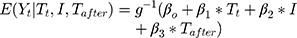
A standard DID model has the following general structure:

where  is the outcome at tth time point for the ith subject, which can be a continuous, binary or count variable;
  is a set of time-varying covariates;
  is a dummy variable indicating pre-post intervention; and
  is a treatment-control indicator variable.14 Parameter
  is the DID intervention effect estimand. Link function
  relates the expected value of the outcome to the predictors in a linear form. In a model with an identity link for a continuous outcome, δ represents the difference of the expected mean difference in the outcome between the two groups comparing pre-intervention to post-intervention, keeping covariates Xit fixed. In the setting of a binary outcome where the logit link is used, δ is interpreted as the difference in log odds of the outcome; when the outcome is a count variable and a Poisson model with log link is used, δ is interpreted as the change in log relative risk of having the outcome.15 In general, if δ is significantly different from zero, this indicates that the intervention has a significant effect on the outcome of interest.
If the assignment of treatment is randomly conditional on time and group fixed effects, ordinary least squares (OLS) regression is an appropriate method for estimation of DID parameters and it is often used in repeated cross-sectional data.16 Because measurements within subjects are repeated over time in panel data, methods to account for the correlated nature of the data are necessary for statistical testing.16 A mixed effects model with a random intercept term is a flexible model which can be used to account for within-subject correlation.17 Alternatively, a generalized estimating equation (GEE) approach can be adopted with a specified working correlation structure, such as autoregressive.18
Assumptions/Model Extensions
The validity of the DID model relies on a few key assumptions. The first is the parallel trend assumption, which asserts that the difference between the two groups is constant over time in the absence of treatment; this assumption is unverifiable using the observed data, and the plausibility of the assumption must be addressed in theoretical terms.14 In practice, researchers often attempt to rely on statistical tests such as including a group-specific linear trend and using a graphic examination to empirically evaluate the credibility of the parallel trend assumption.9,12 While the DID method inherently controls for time-invariant covariates, failure to measure and control for time-varying covariates can lead to erroneous conclusions.19,20 An additional assumption is that there are no spillover effects. Spillover effects occur when aspects of the intervention spill over and affect the control group.21,22 For example, a pay for performance program that incentivizes eligible physicians to increase cancer screening rates may influence non-eligible physicians, especially when eligible and non-eligible physicians practice at the same clinic and/or healthcare facilities. In addition, analysts are required to make standard regression model assumptions.
The DID model can be augmented to adapt to more complex settings. For instance, when serial correlation occurs in the residuals, parametric methods that specify an autocorrelation structure for the error term, or block bootstrap, can be considered.16 When the parallel-trend assumption does not hold, flexible specifications can be introduced to account for the differing trends, such as DID with a group-specific time trend, or a fully flexible DID which makes no parametric assumptions about the time trends for two groups in the absence of the intervention.23 Similarly, when there are case-mix differences across groups or across time, propensity score-based DID models can be considered;12,24,25 for example, inverse probability weighting based on the estimated propensity score can be used instead of directly conditioning on covariates Xit in the DID model.12,24,25
Sample Size Requirements
The DID method does not require a lengthy observation period. In general, sample size requirements depend on the sample ratio of treated to control participants, the magnitude of the intervention effect, the variability of the data, and the correlation between pre- and post-intervention measures.15
Strengths and Limitations
The DID model is easy to implement, since software such as SAS and R have packages and/or procedures that readily fit these models. Regression parameters are straightforward to interpret and the model allows for adjustment of factors that may influence the trend in the outcome over time, if these factors are observed and quantified. Furthermore, the DID model has minimal requirements in terms of the number of observations; in theory, it only requires data from two points in time per group. However, to check the pre-intervention parallel trend assumption, several pre-intervention time periods are useful. A potential limitation of the standard DID model is that it does not allow for a time-varying intervention. Additionally, the DID study design is quasi-experimental; therefore, estimates are subject to threats to internal validity, potentially including selection bias, history bias, and maturation bias.26,27 Selection bias refers to differences between the treated and control groups which, when not properly accounted for, can result in biased effect estimates. History bias refers to events other than the intervention occurring during the study window that may influence the study outcome. Maturation bias can occur when the population changes over time, and these changes are not accounted for in the analysis. As discussed above, another limitation is that the parallel trend assumption is not verifiable using collected data.
Segmented Regression of Interrupted Time Series (ITS)
Segmented regression of interrupted time series (ITS) analysis is another quasi-experimental approach for evaluating the impact of an intervention. In segmented regression analyses of ITS data, the magnitude and constancy of the change in an outcome following an intervention is estimated.
Data Structure
Typically, this method requires ITS data, which are separated by the intervention into segments. In an ITS with only two segments, the first segment contains a series of outcomes measured prior to the intervention, followed by the second segment which contains a series of post-intervention outcomes. Outcomes are aggregated and arranged over a period of time, for example, the proportion of subjects with a certain characteristic of interest, where the proportion is measured repeatedly over time. The unit of analysis in time series studies usually depends on the measurement frequency, which can be daily, weekly, monthly, quarterly or yearly.
Model Specification
A standard segmented regression of ITS model is specified as:
where  is the outcome at time t,
  is a time variable which takes value 1 at the beginning of the observation window and increases with time;
  is a dummy variable indicating whether the observation was measured after the intervention,
 is a time variable which counts the number of periods since the intervention and
  is a link function. Parameter
  is interpreted as the change in the level of the outcome immediately following the intervention, and
  is the change in the trend of the outcome.28
Assumptions/Model Extensions
The following assumptions are made in a segmented regression of ITS analysis: (i) the trend over time is linear; (ii) the cohort’s characteristics remain unchanged through the study period; and (iii) the residuals are independent.11 Assumption (ii) is important because it asserts that in the counterfactual scenario, which is the hypothetical setting where the intervention did not occur, the level and trend in the outcome remains unchanged. This counterfactual scenario serves as the comparison for the observed post-intervention level and trend. Standard segmented regression models can be extended to ensure the robustness of the analysis when deviation from the standard model (2) arises due to a lagged effect, multiple change points, autocorrelation, inclusion of a comparison group, and seasonality. We summarize the model extensions below:
- Lagged effect: The intervention may have a delayed effect, where a change in the trend of the outcome is observed in one or more time periods after the intervention. Failing to account for such a delay can lead to erroneous effect estimates. In practice, lag periods are often excluded from analyses or incorporated as another segment in the model.28,29
- Multiple change points: Interventions can be introduced slowly over multiple time points. Oftentimes a plan to introduce an intervention is announced at one time point, and formally implemented some time later. In these cases, it may be appropriate to specify more than one intervention indicator variable in the regression. For example, the study period can be separated into three intervals, and model (2) can be extended as

Here,  and
and  are interpreted as the changes in level and trend of the outcome after the second intervention, respectively.
- Autocorrelation: Standard segmented regression of ITS fits a least squares regression line in each segment and assumes that the error terms are uncorrelated. The Durbin-Watson test is often used to test for autocorrelation, along with a visual assessment of the autocorrelation function (ACF) and partial autocorrelation function (PACF) plots.29–31 To account for residual autocorrelation, an autoregressive term can be incorporated in the model. Alternatively, a Newey-West adjustment of the standard errors from OLS may be used.32 More complicated models, such as Prais regression or ARIMA, can also be considered; ARIMA models are discussed in detail in the following section.33,34
- Comparison group: The standard ITS design does not have a control group. Assuming that there are no factors other than the intervention affecting the outcome, the counterfactual value serves as the comparison/control. This assumption is less plausible in complex healthcare settings, where more than one intervention or exposure over a period of time is likely. Therefore, investigators may choose to include a comparable control group, assuming the other factors affect both treatment and control groups in a similar way. This is referred to as comparative segmented regression of ITS.25,35 With the introduction of a control group, the model (2) is extended as:
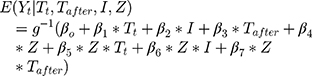
where  is a treatment group indicator variable. Here,
  denotes the difference in the pre-intervention responses between the two groups,
  denotes the difference in the pre-intervention response trend,
  denotes the change in the level differences between groups post-intervention, and
  denotes the change in the trend differences between groups post-intervention.25,29,35,36 Analysts may attempt to balance covariates between groups based on observed pre-intervention data using techniques such as the propensity score weighting described by Linden and Adams.35
- Seasonality: When the outcome under consideration exhibits nonstationary patterns, such as seasonality (annual periodicity within a time series) or cyclicity (long wave swings), characteristics of the patterns must be identified, removed, or modeled before the impact of the intervention can be analyzed. Failing to control for these patterns can obscure the signal and lead to biased estimates. For example, a sudden change in the level of outcomes may be due to a shift in deterministic seasonality or a local trend; alternatively, the lack of a significant change in the outcome after the intervention may be due to the same phenomena. Therefore, removing the effect of seasonality is necessary to separate the true intervention effect from seasonal fluctuations. There are a range of methods for controlling for these patterns: inclusion of an indicator variable for the time period (calendar month or quarter); seasonal differencing; the use of more complex functions such as Fourier terms (pairs of sine and cosine functions) or splines.29 Seasonal ARIMA (SARIMA) models with an interventional component can also be used, which will be discussed in detail in the following section.
Sample Size Requirements
In general, the recommended number of observations for segmented regression of ITS is 12 time points before and 12 time points after the intervention;28 sample size requirements depend on the effect size; the degree of autocorrelation; and whether a level change, trend change, or both are estimated.37
Strengths and Limitations
In general, segmented regression of ITS is straightforward to implement and the parameters are easily interpreted. The data structure is simply a series of aggregate-level outcome measures that are evenly spaced. These types of data are easier to access, since patient and/or physician identifiers are not needed. However, one major limitation is that this method cannot account for complex patterns of nonstationarity. The ARIMA (SARIMA) model is frequently recommended when these patterns exist. In addition, a linear trend might not be realistic, especially when seasonality or cyclic patterns exist. More complex approaches can be implemented to account for non-stationarity or seasonality, such as the use of a spline function; however, this can create challenges in fitting the data, validating model assumptions, and interpreting results.
Interventional Autoregressive Integrated Moving Average (ARIMA) or Seasonal ARIMA (SARIMA) Models
The interventional ARIMA model is another type of model for analysis of ITS data in evaluating the impact of an intervention. The ARIMA model was developed by Box and Jenkins to describe the changes in a series of measurements over time.38 The ARIMA model with intervention was developed to estimate the effect of an intervention while controlling for autocorrelation. It consists of an ARIMA model determined by pre-intervention observations and an intervention function.
Data Structure
The data analyzed in interventional ARIMA (SARIMA) models are ITS data. The unit of analysis is the same as in segmented regression of ITS, which can be daily, weekly, monthly, quarterly or yearly.
Model Specification
In contrast to DID and segmented regression of ITS, ARIMA models are less familiar to clinical researchers. ARIMA models are generally denoted as ARIMA(p,d,q), where parameter p is the order of the autoregressive process, d is the degree of differencing, and q is the order of the moving average process. These parameters are non-negative integers. For example, 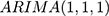 is expressed as:

SARIMA models are usually denoted as ARIMA(p,d,q)(P,D,Q)m, where m refers to the number of periods in each season, and the uppercase P,D,Q refer to the autoregressive, differencing, and moving average terms for the seasonal parts of the ARIMA model. For example, ARIMA(0, 1, 1)(0, 1, 1)12 is expressed as
The ARIMA (SARIMA) model can accommodate autocorrelation, seasonality, and other patterned fluctuations in outcomes. Instead of assuming the time series is linear, as in a simple segmented ITS regression, ARIMA (SARIMA) models attempt to capture temporal structures. Moreover, the intervention analysis in the ARIMA model is not restricted to modelling changes in level and slope only; instead, it can be used to assess more complex patterns that occur as a result of the intervention.
In general, the ARIMA model with an intervention component is formulated as:
Where  is the time series outcome measured at time t,
  is the pre-intervention ARIMA model and
  ) is the intervention function at time t.39,40 The intervention can be a short-term event, such as a short-term advertising campaign to increase product sales; it can also be long-term, such as a change to physician practice guidelines. The intervention function can be chosen to accommodate different scenarios: 1) abrupt onset, permanent duration; 2) abrupt onset, temporary duration; 3) gradual onset, permanent duration; or 4) gradual onset, and gradual decay. Generally, the intervention function can be classified as a step or an impulse function.40 For example, a step function can be formulated as
where 

 - … -
- … -  ; here,
  is the magnitude of the rise or drop of the series,
  is the lag operator,
  is the indictor of intervention,
  is the delay parameter,
  is the speed of the rise or drop.40,41 Details regarding modelling techniques can be found in several texts.41,42
Assumptions/Model Extensions
The main assumption in the ARIMA model with intervention is that the pre-intervention process is “stable” in the sense that the process would have continued in the same way in the counterfactual setting where the intervention did not occur. In other words, it assumes that any changes to the time series stem from the intervention itself. Similar to segmented regression of ITS, a standard interventional ARIMA model requires the assumption that the characteristics of the cohort studied remain unchanged throughout the study period. Analysts must properly specify the p, d, q parameters of the pre-intervention time series to ensure that the residuals are independent.41,42 When seasonality or cyclic patterns arise in the data, the ARIMA model is usually extended to a SARIMA model.
Sample Size Requirements
The ARIMA model generally requires more time points than a segmented regression of ITS, depending on the specific modelling approach and the intervention function.38 For standard interventional ARIMA, the rule of thumb is at least 50 pre-intervention observations, and preferably more than 100 pre-intervention observations.40 Proper modeling of seasonality trends may require even more observations.41 For example, if the time series has a yearly seasonality trend, observations should span enough years to model the seasonality accurately.
Strengths and Limitations
Compared to segmented regression of ITS, the interventional ARIMA (SARIMA) model has several advantages. Analysts can identify and control for seasonality or other nonstationary patterns, such as a sudden level shift caused by seasonal fluctuations, which are often ignored in simple segmented regressions. Residual autocorrelation can be handled or removed by properly specifying the degree of difference, and autoregressive and moving average parameters in an ARIMA model. Instead of assuming that the shape of the impact is linear, the intervention analysis can model different patterns of the impact by specifying different parameters in the intervention function, particularly when the impact is assumed to have a gradual decay form.
Compared to standard segmented regression of ITS, the ARIMA model does have several disadvantages. The modelling process of ARIMA (SARIMA) can be complicated, in particular when selecting p,d,q and P,D,Q. The ACF, the inverse autocorrelation function (IACF), and the PACF are typically used to confirm appropriateness of the model’s parameters and seasonality components.43 ARIMA models may be more likely to be afflicted with instrumentation bias.44,45 Instrumentation bias refers to bias in the intervention analysis estimates caused by changes over time in the way that the outcome is measured/quantified, which can occur over long periods of time. Also, another potential threat to the validity of ARIMA models is that the instrumentation is not calibrated to the appropriate unit of measurement. For example, if the time series has a monthly pattern, while the interval of measurement is quarterly, the pattern may not be detectable or properly accounted for. Unlike DID and comparative segmented regression of ITS, a comparison group cannot be included in an ARIMA model by adding group indicators, since different characteristics of each series determine the p,d,q ARIMA parameters. Instead, the model compares the post-intervention responses to the forecasted values from the pre-intervention ARIMA model.
Table 1 contains a summary of characteristics of the three methods that can be used to guide which model is most suitable for assessing the impact of an intervention.
 |
Table 1 Summary of Study Design, Data Requirements, Assumptions and Extensions of Three Statistical Approaches for Modelling the Impact of an Intervention |
Results
Example 1: The Impact of Medicaid Expansion on Health Insurance Coverage in a Low-Income Population
Expansion of Medicaid coverage for low-income Americans living below 138% of the federal poverty level is one of the key goals of the Affordable Care Act, which was signed into law in 2010.46 Implementation of the Medicaid expansion depended on state-level decisions.47 On January 1, 2014, 25 states expanded their Medicaid eligibility and two expanded later in 2014. An additional 5 states implemented expansions in 2015 and 2016. By September 2016, 32 states had expanded Medicaid coverage while the remaining 19 states opted not to. We evaluated the impact of Medicaid expansion on insurance coverage among low-income populations by comparing states with and without expanded coverage.
We derived the prevalence of health insurance coverage for each state from the 2012–2017 Behavioral Risk Factor Surveillance System (BRFSS), which collects data from US adults in each state regarding health-related risk behaviors, chronic health conditions, and access to healthcare, including health insurance. Survey respondents, while representative for each state, differ from year to year. Other studies have investigated the impact of Medicaid expansion at the individual level,48–50 whereas we utilize state-level data, where each state is the subject of analysis. The yearly prevalence of insurance coverage is calculated as the weighted proportion of those who answered “yes” to any type of insurance coverage among all respondents whose annual family income is below $35,000 in each state, since this subset was expected to show the most significant impact regarding access to healthcare in the expansion states.51–53 All state-level covariates are from the Centers for Disease Control and Prevention, including the proportion of black, Hispanic, female, and older (age ≥65 years) residents.54 The proportion of those who are poor and living in poverty was calculated from Census Bureau data.55 The schedule of expansion for each state was extracted from data compiled by the Kaiser Family Foundation.56
The available data are panel data, with each state as the cross-sectional unit, and only six yearly measurements are in the study window; state-specific covariates are available, and an appropriate comparison group is also available. Therefore, we used the DID model, specified as equation (1) with an identity link to compare the change in health insurance coverage before and after Medicaid expansion between the two groups of states, controlling for the state-level covariates noted above. We defined the treatment group as states with expanded Medicaid coverage by September 2016, while the control group included states without Medicaid expansion before September 2016. We defined the pre-intervention period as the years 2012–2013, and the post-intervention period as the years 2014–2017. To account for unobserved factors which may have influenced the decision for a state to join the expansion, we included state fixed effects in the DID regression. We also performed sensitivity analyses using 1) DID with a linear time trend, 2) DID with both a linear trend and state-fixed effect, and 3) propensity score-weighted DID with a state fixed-effect. We also present the results of a pre-trend test of interaction of time and treatment to examine the pre-intervention parallel trend assumption.
Estimates from these models are shown in Table 2. Medicaid expansion increased insurance coverage in the low-income population (Figure 1). The fixed-effect estimate shows an increase of 5.93 (95% CI, 3.99 to 7.89) percentage points in the difference of health insurance coverage between two groups in the post-expansion period compared to the pre-expansion period, slightly higher than the estimates from the state fixed-effect DID model with a linear trend (5.47, 95% CI,4.05 to 7.86) and close to the propensity score-weighted estimate (5.95, 95% CI, 4.05 to 7.86). The tests of the parallel trend assumption show that the null hypothesis of a common trend holds for all models.
 |
Table 2 Estimated Impact of Medicaid Expansion on Health Insurance Coverage Under Different DID Models |
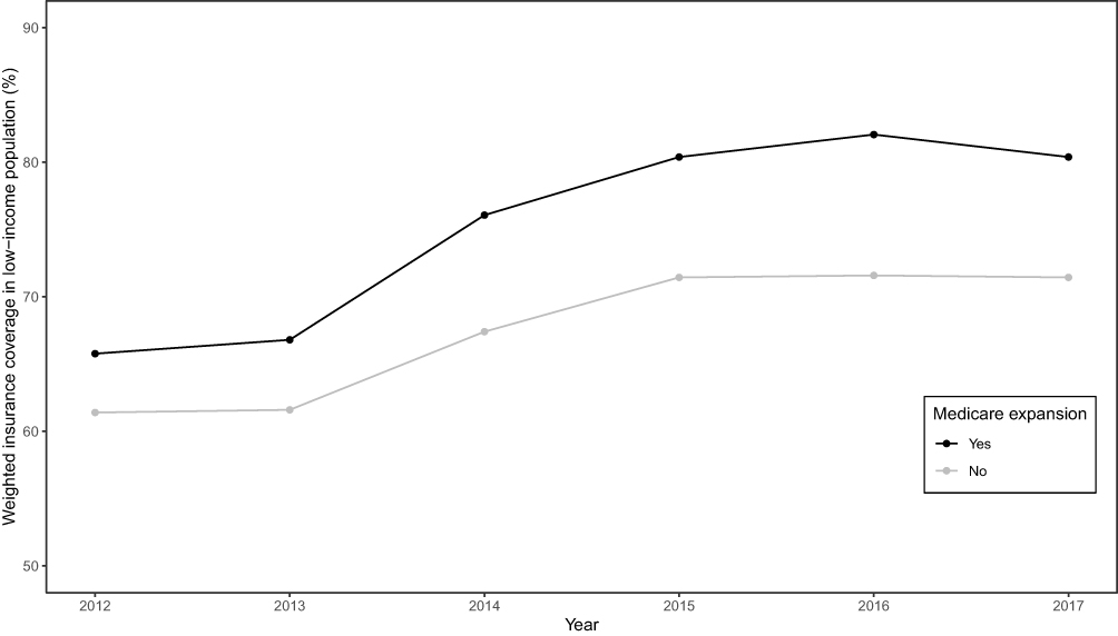 |
Figure 1 Trend in health insurance coverage in a low-income population in the United States from 2012 to 2017. |
Example 2: Assessment of Impact of a Clinical Decision Support Tool in Increasing Appropriateness Score of High-Cost Imaging Orders
Electronic medical record (EMR)-embedded clinical decision support tools are recommended by Center for Medicare and Medicaid (CMS) to improve the appropriateness of ordering high-cost imaging tests such as CT scans, PET scans, and MRI. Since April 2013, a digital version of the American College of Radiology (ACR) Appropriateness Criteria, ACR Select, was embedded in our tertiary care hospital’s EMR system, and all providers in inpatient and emergency department settings are required to use it when placing a diagnostic imaging order.57 The ACR Select calculates a score between 1 and 9 which describes the increasing appropriateness of the imaging order corresponding to higher scores. When a score of 5 or less is computed, a best practice alert pops up with ACR Select content, which advises that the provider choose a more appropriate scan and shows recommended alternatives. This ACR Select scoring tool was implemented with a best practice alert in silent mode in April 2013 and put in live mode from April 2015.
We analyzed the hospital data from April 2013 to June 2016, hypothesizing that the appropriateness scores would be improved in the emergency department setting but not in the inpatient setting. Our rationale for this hypothesis was that only emergency department physicians were given continuing education to inform them about the value of the ACR Select tool. The outcome of interest was the mean ACR Select tool appropriateness score, computed at monthly intervals and stratified by treatment setting (emergency department vs. inpatient). We considered April 2015 as the start date for the intervention.
The data used in this example are time series data in nature; therefore, we have chosen not to use DID which is typically used with panel data. In addition, seasonality is not observed, and an appropriate comparison group is available; therefore, we have chosen to use comparative segmented regression of ITS rather than ARIMA to test our hypothesis. We used equation (4) with an identity link to fit the data. The Durbin-Watson statistic was used to test for serial autocorrelation of the residuals. The ACF and PACF of the residuals were plotted to visually explore residual autocorrelation, and to identify the order of lag.
The level of difference in appropriateness scores between emergency department and inpatient settings before the alert began was −0.22 (95% CI, −0.31 to −0.12); the mean score was 6.58 in the inpatient setting and 6.36 in the emergency department (Table 3). The trend difference before the intervention was −0.01 (95% CI, −0.02 to −0.01), with a trend of 0.01 for the inpatient setting and −0.002 for the emergency department setting. After the intervention, the mean score in the emergency department exceeded that in the inpatient setting with a change in the level of 0.63 (95% CI, 0.53 to 0.73) and a change in trend of 0.02 (95% CI, 0.01 to 0.03) (Figure 2), suggesting that the ACR Select tool had a significant impact on providers in choosing appropriate imaging tests in the emergency department setting. However, the significant decrease in mean ACR appropriateness score in the inpatient setting may have been caused by another event, such as recruitment of few senior radiologists during this time interval, signaling potential history bias. In addition, the estimate of impact may also be subject to selection bias, for example, the differences in provider practices between settings (e.g., case-mix of their patients) may have “explained” some of the difference in the appropriateness scores.
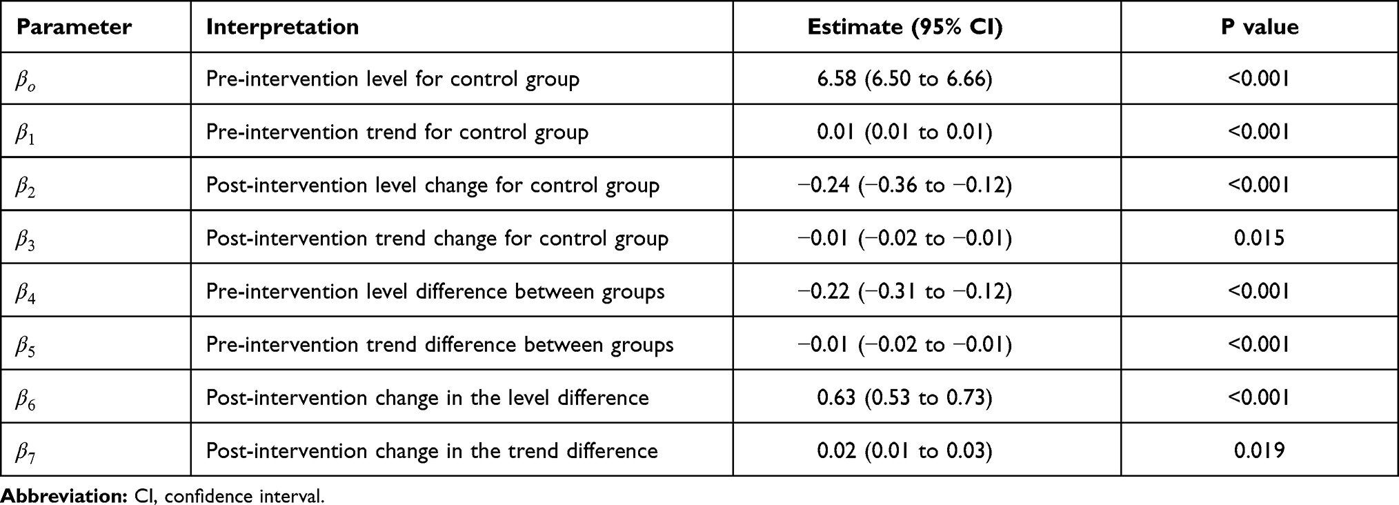 |
Table 3 Estimates from a Comparative Segmented Regression of ITS Analysis for Assessing the Impact of an ACR Select Tool in Increasing the Mean Appropriateness Score of High-Cost Imaging Orders |
 |
Figure 2 Mean scores and predicted regression line for appropriateness scores of imaging orders in an emergency department setting versus an inpatient setting over time. Abbreviation: ED, emergency department. |
The Durbin-Watson test statistic is 2.15, showing no significant positive autocorrelation (P=0.553) and no significant negative autocorrelation (p=0.446). The ACF and partial PACF plots confirm that there is no significant autocorrelation with any lagged term and no order of lag term is identified (Appendix Figure A1). Therefore, we did not consider the Newey-West approach to adjust the standard error or consider autoregressive models.32
Example 3: The Effects of eGFR Reporting with Prompts on Physician Requests for Creatinine Clearance Collection in Ontario, Canada
In January 2006, all outpatient laboratories in Ontario, Canada began reporting estimated glomerular filtration rate (eGFR), a measure of kidney function which determines the stage of kidney disease, whenever a serum creatinine test was ordered.58 The Canadian Society of Nephrology endorsed the routine usage of eGFR reporting in patients with chronic kidney disease in the same year.59 To better understand the influence of such initiatives on clinician practice, we sought to examine the effects of the population-wide introduction of eGFR reporting with prompts on physician ordering of 24-hour urine collection for creatinine clearance.5
We obtained aggregate-level data from the author’s previous publication. The outcome of interest was the age- and sex-standardized monthly number of 24-hour creatinine clearance tests per 100,000 Ontario outpatients aged 25 years or older, between July 1999 and July 2009. We defined January 2006 as the intervention date, July 1999 to December 2005 as the pre-intervention period, and January 2006 to July 2009 as the post-intervention period.
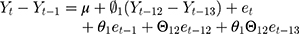
Because strong autocorrelation and a yearly cycle (indicating seasonality) were detected, we used an interventional SARIMA model to estimate the impact of the intervention on the outcome of interest, with an intervention function and a lag time of up to 3 months. This model allowed us to characterize the non-linear change in the numbers of creatinine clearance collections from the pre- to post-eGFR reporting time periods. The SARIMA model was ARIMA (1, 1, 1) (1, 0, 0)12 with intervention function  . Visual examination of the ACF, IACF, and PACF plots confirmed the model parameter appropriateness and seasonality. Model diagnostics were confirmed by examining the autocorrelations at various lags with the Ljung–Box χ2 statistic and residual diagnostic plots (Appendix Figure A2).
The number of creatinine clearance tests decreased significantly within months of the start of eGFR reporting (Figure 3). Although the creatinine clearance tests appeared to decrease slightly in the absence of the intervention (forecasted grey line), the actual number of tests after the intervention dropped even more markedly with a magnitude of drop equal to −0.93 (95% CI, −1.22 to −0.64) tests per 100,000 adults and a rate of drop of 0.97 (95% CI, 0.95 to 0.99) tests per 100,000 per adults per month (Table 4). We note that the estimate may be afflicted with issues that threaten the validity. For example, events other than the population-wide introduction of eGFR reporting may have occurred in the relatively long study window (history bias); also, the characteristics of the study population may have changed during the study window (maturation bias).
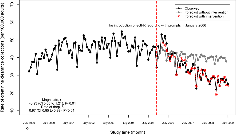 |
Figure 3 Monthly numbers of 24-hour creatinine clearance collections in Ontario, Canada (adjusted for age and sex) and post-intervention forecast value. |
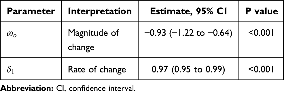 |
Table 4 Parameter Estimates from a SARIMA Model with Intervention in Examining the Effects of eGFR Reporting with Prompts on Physician Requests for Creatinine Clearance Collection in Ontario, Canada |
Discussion
Clear and comprehensive guidance about study design, model specifications, assumptions, sample size requirements, and strengths and limitations of each of the three interventional analysis approaches presented in this article is valuable to practitioners as these methodologies are being rapidly adopted in clinical research.
In this article, we describe three models commonly used for evaluating the impact of an intervention, each with its own strengths, limitations, and underlying assumptions. When choosing the appropriate method to model the intervention effect, considerations include the knowledge of the study design from which the data have emerged, structure of the data, availability of a comparison group, and other patterns in the data. During the design stage, if the study is constrained in time and an appropriate control group is avaiable, DID should be considered . During analysis, the nature of the data and the population observed over time are important considerations. If longitudinal aggregate-level data are available and the population studied is relatively stable, then an interrupted time series design is appropriate, provided there are no factors other than the intervention of interest and a linear time trend is observed; SARIMA should be considered when seasonality or a cyclic pattern is expected in the data.
In addition to appropriate study design and data analysis, appropriate reporting of results is also important. The reporting of effect estimates can differ across the three methods. In DID, the coefficient of the interaction term, also called the DID estimator, is the estimand of interest in most contexts; investigators may also report covariate effects if applicable. In segmented regression of ITS analysis, the changes in the level and trend post-intervention are reported if there is no control group, while the difference in the change in level/trend between groups should be the main focus in a comparative ITS study. In an interventional ARIMA analysis, the reported results typically include a rate parameter (rate of change), a slope parameter (magnitude of change), and a delay parameter, depending on the shape of the intervention function. Reporting guidance and checklists for the three methods reviewed in this article are available.12,31,60
Data Sharing Statement
The Behavioral Risk Factor Surveillance System (BRFSS) data are publicly available and can be found at the website of Centers for Disease Control and Prevention (CDC, https://www.cdc.gov/brfss/index.html). Any aggregate-level data presented in the manuscript can be requested from the corresponding author.
Ethics Approval and Consent to Participate
Ethical approval for the ACR appropriateness score data used in this study was obtained from Icahn School of Medicine at Mount Sinai Program for the Protection of Human Subjects, Institutional Review Boards (reference number HS14–00799). Because the data used in this study are at the aggregated level and therefore do not contain personal identifiers, the need for consent was waived by the IRB. The Behavioral Risk Factor Surveillance System (BRFSS) data and aggregate-level serum creatinine test data are publicly available; therefore, ethical approval is not required.
Author Contributions
Lihua Li and Meaghan S Cuerden are joint first co-authors. All authors made substantial contributions to conception and design, acquisition of data, or analysis and interpretation of data; took part in drafting the article or revising it critically for important intellectual content; agreed to submit to the current journal; gave final approval of the version to be published; and agree to be accountable for all aspects of the work.
Funding
Research reported in this publication was supported in part by the National Cancer Institute Cancer Center Support Grant P30CA196521-01 awarded to the Tisch Cancer Institute (TCI) of the Icahn School of Medicine at Mount Sinai (IS-MMS). LL, MM are member of the Biostatistics Shared Resource Facility for TCI-ISMMS and were provided support for this project in terms of protected time. Research reported in this publication was also supported in part by the National Institute of Aging grants P30AG028741 and AG028741 awarded to the Pepper Older Americans Independence Center of the Icahn School of Medicine at Mount Sinai (IS-MMS). The funder had no role in study design, data collection and analysis, decision to publish, or preparation of the manuscript.
Disclosure
The authors declare that they have no conflict of interests for this work.
References
1. Nayor M, Vasan RS. Recent update to the US cholesterol treatment guidelines. Circulation. 2016;133(18):1795–1806. doi:10.1161/CIRCULATIONAHA.116.021407
2. McFarland DC, Shen M, Harris K, et al. ReCAP: would women with breast cancer prefer to receive an antidepressant for anxiety or depression from their oncologist? J Oncol Pract. 2016;12(2):172–174. doi:10.1200/JOP.2015.006833
3. Garg P, Ko DT, Jenkyn KMB, Li L, Shariff SZ. Infective endocarditis hospitalizations and antibiotic prophylaxis rates before and after the 2007 American Heart Association guideline revision. Circulation. 2019;140(3):170–180. doi:10.1161/CIRCULATIONAHA.118.037657
4. Han B, Yu H. Causal difference-in-differences estimation for evaluating the impact of semi-continuous medical home scores on health care for children. Health Serv Outcomes Res Methodol. 2019;19(1):61–78. doi:10.1007/s10742-018-00195-9
5. Kagoma YK, Garg AX, Li L, Jain AK. Reporting of the estimated glomerular filtration rate decreased creatinine clearance testing. Kidney Int. 2012;81(12):1245–1247. doi:10.1038/ki.2011.483
6. Lam M, Li L, Anderson KK, Shariff SZ, Forchuk C. Evaluation of the transitional discharge model on use of psychiatric health services: an interrupted time series analysis. J Psychiatr Ment Health Nurs. 2020;27(2):172–184. doi:10.1111/jpm.12562
7. Kolstad JT, Kowalski AE. The impact of health care reform on hospital and preventive care: evidence from Massachusetts. J Public Econ. 2012;96(11):909–929. doi:10.1016/j.jpubeco.2012.07.003
8. Emmanuel O, Adebanji A, Glele Kakaï RL. ARIMA-noise model for a segmented intervention analysis of maternal health policy on assisted delivery. Int J Appl Math Stat. 2014;52:62–71.
9. Saeed S, Moodie EEM, Strumpf EC, Klein MB. Evaluating the impact of health policies: using a difference-in-differences approach. Int J Public Health. 2019;64(4):637–642. doi:10.1007/s00038-018-1195-2
10. Sanson-Fisher RW, D’Este CA, Carey ML, Noble N, Paul CL. Evaluation of systems-oriented public health interventions: alternative research designs. Annu Rev Public Health. 2014;35(1):9–27. doi:10.1146/annurev-publhealth-032013-182445
11. Kontopantelis E, Doran T, Springate DA, Buchan I, Reeves D. Regression based quasi-experimental approach when randomisation is not an option: interrupted time series analysis. BMJ. 2015;350(jun09 5):h2750. doi:10.1136/bmj.h2750
12. Wing C, Simon K, Bello-Gomez RA. Designing difference in difference studies: best practices for public health policy research. Annu Rev Public Health. 2018;39(1):453–469. doi:10.1146/annurev-publhealth-040617-013507
13. Zeger SL, Irizarry R, Peng RD. On time series analysis of public health and biomedical data. Annu Rev Public Health. 2006;27(1):57–79. doi:10.1146/annurev.publhealth.26.021304.144517
14. Kahn-Lang A, Lang K. The promise and pitfalls of differences-in-differences: reflections on 16 and pregnant and other applications. J Bus Econ Stat. 2020;38(3):613–620.
15. E Margaret Warton MMP. Oops, I D-I-D It Again! Advanced Difference-In-Differences Models in SAS. Western Users of SAS® Software; 2016.
16. Bertrand M, Duflo E, Mullainathan S. How much should we trust differences-in-differences estimates? Q J Econ. 2004;119(1):249–275. doi:10.1162/003355304772839588
17. Wolfinger R, Chang M Comparing the SAS® GLM and MIXED procedures for repeated measures.
18. Hansen CB. Generalized least squares inference in panel and multilevel models with serial correlation and fixed effects. J Econom. 2007;140(2):670–694. doi:10.1016/j.jeconom.2006.07.011
19. Zeldow B, Hatfield LA. Confounding and regression adjustment in difference-in-differences. arXiv. 2019;arXiv:
20. Keele LJ, Small DS, Hsu JY, Fogarty CB. Patterns of effects and sensitivity analysis for differences-in-differences. arXiv. 2019;arXiv:
21. Miguel E, Kremer M. Worms: identifying impacts on education and health in the presence of treatment externalities. Econometrica. 2004;72(1):159–217. doi:10.1111/j.1468-0262.2004.00481.x
22. Lechner M. The estimation of causal effects by difference-in-difference methods. Found Trends Microecon. 2011;4(3):165–224. doi:10.1561/0800000014
23. Mora R, Reggio I. Treatment Effect Identification Using Alternative Parallel Assumptions. Universidad Carlos III de Madrid. Departamento de Economía; December, 2012.
24. Stuart EA, Huskamp HA, Duckworth K, et al. Using propensity scores in difference-in-differences models to estimate the effects of a policy change. Health Serv Outcomes Res Methodol. 2014;14(4):166–182. doi:10.1007/s10742-014-0123-z
25. Linden A, Adams JL. Applying a propensity score-based weighting model to interrupted time series data: improving causal inference in programme evaluation. J Eval Clin Pract. 2011;17(6):1231–1238. doi:10.1111/j.1365-2753.2010.01504.x
26. Handley MA, Lyles CR, McCulloch C, Cattamanchi A. Selecting and improving quasi-experimental designs in effectiveness and implementation research. Annu Rev Public Health. 2018;39(1):5–25. doi:10.1146/annurev-publhealth-040617-014128
27. Cook TD, Campbell DT. Quasi-Experimentation: Design and Analysis Issues for Field Settings. Houghton Mifflin; 1979.
28. Wagner AK, Soumerai SB, Zhang F, Ross-Degnan D. Segmented regression analysis of interrupted time series studies in medication use research. J Clin Pharm Ther. 2002;27(4):299–309. doi:10.1046/j.1365-2710.2002.00430.x
29. Bernal JL, Cummins S, Gasparrini A. Interrupted time series regression for the evaluation of public health interventions: a tutorial. Int J Epidemiol. 2017;46(1):348–355. doi:10.1093/ije/dyw098
30. Lagarde M. How to do (or not to do) assessing the impact of a policy change with routine longitudinal data. Health Policy Plan. 2011;27(1):76–83. doi:10.1093/heapol/czr004
31. Hudson J, Fielding S, Ramsay CR. Methodology and reporting characteristics of studies using interrupted time series design in healthcare. BMC Med Res Methodol. 2019;19(1):137. doi:10.1186/s12874-019-0777-x
32. Newey WK, West KD. A simple, positive semi-definite, heteroskedasticity and autocorrelation consistent covariance matrix. Econometrica. 1987;55(3):703–708. 10.2307/1913610
33. S. J. Prais CBW. Trend estimators and serial correlation. Cowles Commission discussion paper Stat No 383. 1954.
34. Nelson BK. Time series analysis using Autoregressive Integrated Moving Average (ARIMA) models. Acad Emergency Med. 1998;5(7):739–744. doi:10.1111/j.1553-2712.1998.tb02493.x
35. Linden A. Conducting interrupted time-series analysis for single- and multiple-group comparisons. Stata J. 2015;15(2):480–500. doi:10.1177/1536867X1501500208
36. Simonton DK. Erratum to simonton. Psychol Bull. 1977;84(6):1097. doi:10.1037/h0078052
37. Zhang F, Wagner AK, Ross-Degnan D. Simulation-based power calculation for designing interrupted time series analyses of health policy interventions. J Clin Epidemiol. 2011;64(11):1252–1261. doi:10.1016/j.jclinepi.2011.02.007
38. Box GEP, Jenkins G. Time Series Analysis, Forecasting and Control. Holden-Day, Inc.; 1990.
39. Hibbs JDA. On analyzing the effects of policy interventions: Box-Jenkins and Box-Tiao vs. structural equation models. Sociol Methodol. 1977;8:137. doi:10.2307/270755
40. Box GEP, Tiao GC. Intervention analysis with applications to economic and environmental problems. J Am Stat Assoc. 1975;70(349):70–79. doi:10.1080/01621459.1975.10480264
41. Yaffee R, McGee M. An Introduction to Time Series Analysis and Forecasting with Applications of SAS® and SPSS®.
42. Hyndman RJ, Athanasopoulos G. Forecasting: Principles and Practice.
43. Crabtree BF, Ray SC, Schmidt PM, O’Connor PJ, Schmidt DD. The individual over time: time series applications in health care research. J Clin Epidemiol. 1990;43(3):241–260. doi:10.1016/0895-4356(90)90005-A
44. Linden A. Challenges to validity in single-group interrupted time series analysis. J Eval Clin Pract. 2017;23(2):413–418. doi:10.1111/jep.12638
45. Biglan A, Ary D, Wagenaar AC. The value of interrupted time-series experiments for community intervention research. Prev Sci. 2000;1(1):31–49. doi:10.1023/A:1010024016308
46. U.S. Department of Health and Human Services. Compilation of Patient Protection and Affordable Care Act. 2010. 2010.
47. Status of State Action on the Medicaid Expansion Decision. Kaiser Family Foundation. Available from: http://www.kff.org/health-reform/state-indicator/state-activity-around-expanding-medicaid-under-the-affordable-care-act/.
48. Benitez JA, Creel L, Jennings JA. Kentucky’s medicaid expansion showing early promise on coverage and access to care. Health Aff. 2016;35(3):528–534. doi:10.1377/hlthaff.2015.1294
49. Blavin F, Karpman M, Kenney GM, Sommers BD. Medicaid versus marketplace coverage for near-poor adults: effects on out-of-pocket spending and coverage. Health Aff. 2018;37(2):299–307. doi:10.1377/hlthaff.2017.1166
50. Cawley J, Soni A, Simon K. Third year of survey data shows continuing benefits of medicaid expansions for low-income childless adults in the U.S. J Gen Intern Med. 2018;33(9):1495–1497. doi:10.1007/s11606-018-4537-0
51. Martinez M, Ward B. Health care access and utilization among adults aged 18–64, by poverty level: United States, 2013–2015. NCHS Data Brief. 2016;262:1–8.
52. Sommers BD, Blendon RJ, Orav EJ, Epstein AM. Changes in utilization and health among low-income adults after medicaid expansion or expanded private insurance. JAMA Intern Med. 2016;176(10):1501–1509. doi:10.1001/jamainternmed.2016.4419
53. Sommers BD, Gunja MZ, Finegold K, Musco T. Changes in self-reported insurance coverage, access to care, and health under the affordable care act. JAMA. 2015;314(4):366–374. doi:10.1001/jama.2015.8421
54. Centers for Disease Control and Prevention. Bridged-race population estimates 1990–2017 request. Available from: https://wonder.cdc.gov/bridged-race-v2017.html.
55. Table 21. Number of poor and poverty rate, by state: 1980 to 2018. Available from: https://www2.census.gov/programs-surveys/cps/tables/time-series/historical-poverty-people/hstpov21.xls/.
56. Kaiser Family Foundation. Status of state medicaid expansion decisions: interactive map. Available from: https://www.kff.org/medicaid/issue-brief/status-of-state-medicaid-expansion-decisions-interactive-map/.
57. Poeran J, Mao LJ, Zubizarreta N, et al. Effect of clinical decision support on appropriateness of advanced imaging use among physicians-in-training. Am J Roentgenol. 2019;212(4):859–866. doi:10.2214/AJR.18.19931
58. Jain AK, McLeod I, Huo C, et al. When laboratories report estimated glomerular filtration rates in addition to serum creatinines, nephrology consults increase. Kidney Int. 2009;76(3):318–323. doi:10.1038/ki.2009.158
59. Levin A, Mendelssohn D. Care and referral of adult patients with reduced kidney function: position paper from the Canadian Society of Nephrology. Can Soc Nephrol. 2006.
60. Ryan AM, Burgess JF
 © 2021 The Author(s). This work is published and licensed by Dove Medical Press Limited. The
full terms of this license are available at https://www.dovepress.com/terms
and incorporate the Creative Commons Attribution
- Non Commercial (unported, 3.0) License.
By accessing the work you hereby accept the Terms. Non-commercial uses of the work are permitted
without any further permission from Dove Medical Press Limited, provided the work is properly
attributed. For permission for commercial use of this work, please see paragraphs 4.2 and 5 of our Terms.
© 2021 The Author(s). This work is published and licensed by Dove Medical Press Limited. The
full terms of this license are available at https://www.dovepress.com/terms
and incorporate the Creative Commons Attribution
- Non Commercial (unported, 3.0) License.
By accessing the work you hereby accept the Terms. Non-commercial uses of the work are permitted
without any further permission from Dove Medical Press Limited, provided the work is properly
attributed. For permission for commercial use of this work, please see paragraphs 4.2 and 5 of our Terms.