Rain dance: the role of randomization in clinical trials

Introduction

Research controlled experiments often rely on the comparison of end-point responses of two treatments to investigate the efficacy of an intervention. For the experiment to be fruitful, the samples ought to be comparable. The researcher should aim for samples that differ – up to his knowledge – solely on the respective allocated treatments. Differences on the responses therefore shall be (tentatively) attributed exclusively to the effect of treatments. For decades, the preferential method for selecting samples that should be balanced for clinical trials has been based on different methods of randomization.

The introduction of randomization as a method of allocation was a benchmark in the evolution of modern clinical trials and became a gold standard for testing the efficacy of treatment interventions.¹ However, despite its undisputed importance, randomization is not flawless.² Given that any sample can result from randomization, it may generate samples that are not balanced regarding baseline characteristics and putative prognostic factors. Therefore, randomization does not necessarily generate samples that are suitable for determining the comparative efficacy of interventions.

Postponing or even totally avoiding randomization is not a new idea in Statistical Design of Experiments. It started as early as 1971 and was contemplated by different authors. For more information, see Basu,^3–5 Brewer,⁶ Berry and Kadane,⁷ DasGupta,⁸ Kadane and Seidenfeld,⁹ and Ware.¹⁰

The attempts to control for the imbalances that may be produced by randomization are also known as minimization methods. For a complete review on these methodologies, please see Scott et al.¹¹ The alternative methods of allocation including minimization procedures that can avoid randomization shortcomings^12–14 are, however, rarely used. The infrequent application of such methods in current clinical trials may be related to the misconceptions regarding the risks of abandoning randomization.

In this article, we use a fictitious case example to illustrate the randomization paradox. We revise and discuss the putative reasons for favoring randomization and evaluate an alternative method of allocation that does not require prior knowledge of the total or any partial sample composition and, therefore, is named sequential allocation.

Figure 1 depicts ancient devices of random allocation.

Figure 1 Primitive randomization devices. Notes: (A) Ovine astragalus bone used for gambling (circa 300 BC). (B) Astragalus monument in Kyrgyzstan. (B) Reproduced from wikimedia.org (http://creativecommons.org/licenses/by-sa/3.0/).40

A fictitious case example to illustrate an everyday paradox in medical research

A clinician named Ed wants to test the benefits of a new dietary supplement advertised as an antiobesity medication in his patients who are overweight. He has 12 patients scheduled for next week in his clinic. He decides to offer the new supplement to six of the patients who happen to also be his friends and leave the other patients with treatment-as-usual. But before running his experiment, Ed consults Joe, his supervisor, who is highly specialized in the field of clinical trials. Joe tells Ed that the idea of dividing his sample in groups of friends and of ordinary patients is unwise and will preclude comparisons between supplements. Joe suggests to Ed that he uses a simple randomization procedure to allocate his patients. Ed agrees and immediately prints the list of all his 12 patients in alphabetical order. Then he gets 12 marbles (numbered from 1 to 12) from the Bingo toy he bought for his son. He and Joe agree that the first six drawn numbers will correspond to the patients receiving the new treatment. It so happens that all his six friend patients are selected (by the Bingo globe) for the new supplement, while the remaining patients will obtain treatment-as-usual, as before. This fictitious case illustrates a paradox: a sample otherwise considered inadequate for an experiment can be the result of a procedure of simple randomization. If Joe deems friendship with Ed a relevant prognostic factor (as, say, friends tend to better comply with treatments prescribed by a buddy-doctor), it is illogical of him not to demand that – prior to any randomization – friends of Ed are equally distributed between interventional groups.

Most researchers will come up with a number of relevant prognostic variables (stratification variables) that will end up dismissing any randomization whatsoever, especially with small total sample numbers (eg, suppose that both friends and nonfriends groups have four male and two female patients who need to be equally distributed between interventional groups to control for the effect of sex, and so on). If, when bias is perceived, randomization is not guaranteed to avoid it, why is one so prone to embrace it?

We consider several objections raised by tradition against the clear and straightforward idea of using intentional allocation in the conduction of real-life clinical trials to achieve more balanced, and therefore comparable, groups.

Overviewing the reasons for randomization held by tradition

Reason A: every sample unit must have the same chance of being selected

According to reason A, bad (unbalanced) and good (balanced) samples should have the same chances of being selected. This very democratic fact about randomization creates the problems that justify restricted randomization. It is exactly because any sample allocation is possible with randomization that poorly balanced and biased samples can often result from endless randomizations. In biased samples, the characteristics that are unbalanced between interventional groups can act as confounding factors, once they may interfere with the result of the study regardless of the intervention being tested.

Some researchers argue that, in the face of a bad sample generated by randomization, it is possible to correct the effect of confounding factors (characteristics that are unbalanced between groups and that could interfere with the results) in posterior analysis. However, to control for confounders, information on the effect of the confounder has to be available. If, as in Ed and Joe’s case, there is no information on the effect of being a friend of the doctor promoting the experiment (because all friends participated only in one arm of the study), reason A becomes untenable. Moreover, if we can diminish the chance of a bad sample, why would we rely on posterior analysis to correct for a problem that could have been easily prevented?

To increase the problem further, the fact that every sample has the same chance of being selected makes it impossible to trace if an unbalanced sample was generated randomly (by accident) or not (eg, in the case of intentional bias). Of note, even when using a method of intentional allocation that is not totally deterministic, it is possible to confirm if one specific allocation result is among the possible results produced by that allocation procedure.

Moreover, when randomizing, scientists create an additional paradox: the paradox of posterior hypothesis testing. Hypothesis testing tells you the probability of a result having occurred by chance. Hence, if it is already known that a difference is the consequence of randomization (pure chance), why should we test whether it has occurred by chance? As a matter of fact, the urge to compare interventional groups to test for “good” balance of prognostic factors points to the fact that ideal allocations should not be strictly random, as many randomized options need to be avoided even if produced by some unbiased randomization device.

Furthermore, somewhat ironically, very well-balanced allocations intentionally chosen could have been produced by simple randomization. Therefore, even if a statistical test is based on the assumption that the sample is a randomly selected subgroup of a population, it is still adequate to analyze intentionally produced samples; given that intentionally produced samples are part of the universe of possibilities of randomly chosen samples.

In conclusion, reason A does not hold in face of the advantages of intentional allocation. Intentional allocation decreases the chance of producing bad random samples, and makes it possible to trace if a specific method was employed for that specific result of allocation. Since intentional allocation does not rely on the availability of information on the effect of unbalanced factors as posterior analyses do, careful balancing promoted by methods of intentional allocation seems much more appropriate than randomization to prevent the effect of confounding factors. In addition, as a bonus, it makes the controversial posterior testing of homogeneity of baseline characteristics of interventional groups unnecessary, undoing the posterior hypothesis testing paradox.

Reason B: randomization avoids human interference in the allocation of patients (while any other form of allocation does not)

Personal interference from scientists is a matter of concern in the design of experiments. In fact, avoidance of “nonrandom” interference in the design is the most voiced and traditional reason for randomizing: even unintentionally, a scientist might “give an artificial (dis)advantage” to some experimental procedure. For example, a physician may submit his new procedure mostly to healthier patients while leaving treatment-as-usual to unhealthier ones, increasing the chances of the new procedure being proved more effective than the traditional one.

The application of not completely random (more deterministic) methods of allocation raises the concern that researchers may gain control over the allocation in order for a specific subject to receive a more desired intervention. That concern is built on the assumption that knowledge of the prognostic factors included in the process enables a researcher to accurately guess the allocation of each subject. Indeed, in some specific minimization methods, it is possible to guess correctly where a subject will be allocated having prior knowledge of the characteristics of the previously allocated subjects.¹¹ In the time-sequential purposive allocation protocol to be described in the section on Evaluating sequential methods as alternatives to randomization, however, it is not the case. In addition, even for the minimization procedures where accurate guesses are indeed possible, there are ways to prevent the certainty about allocation without significant prejudice of the efficiency of the method.¹⁵

In the allocation method described in Section 3, for the first arriving patients, the decision is random and therefore unpredictable. Once there are sufficient (two, usually) sample units to start balancing the baseline characteristics of patients among groups, the next step allocation is decided upon a complex calculation that uses several putative prognostic factors and all the information on previously included patients. Moreover, if allocation in any of the groups produces the same difference between groups, the decision will, once again, be random. The randomness kept in the process and the complexity of the calculations make it practically impossible to guess to which group a patient will be allocated. Therefore, well-built methods of allocation such as the one from Section 3 can make it almost impossible for the researcher to manipulate its results.

Reason C: nonrandom allocation procedures implicate great technical difficulties while providing negligible gains regarding balance between interventional groups

The technical difficulties implied by the application of intentional allocation procedures vary according to the method of allocation. In the method described in Section 3, once the prognostic factors are chosen, the weight for each factor is determined and the calculation of the compositional distance between groups is set, allocating each subject is as simple as it would be in the case of using any process of randomization and much simpler than applying stratification or block procedures. Therefore, with the recent computational developments and the use of a sequential method that does not require prior knowledge about the total or partial sample composition, the argument that intentional allocation implicates great technical difficulties does not hold.

The gains obtained with the use intentional allocation depend on several factors. The most straightforward factor is the sample size. Smaller sample sizes will be the ones to achieve greater benefit given the higher chance of random imbalance. In addition, the existence of well-known prognostic factors with great effect over outcome also will result in greater benefits since the controlled variable during the process of allocation will be a variable of great relevance. Therefore, the gains of intentional allocation have to be determined on an individual basis.

Reason D: if samples are not completely random, classical statistical analysis cannot be performed

Randomization, in combination with blinding of interventions being administered, has been a time-honored antidote against unfair trials. However, as Ed and Joe have shown us, it is an antidote which does not avoid unbalance. In other words, it is not a completely effective antidote.

Even in a trial in which the scientists control all prognostic factors that they believe are relevant, it can happen that they ignore the possible influence of other factors. This could be a reason for – at last – randomizing. If, however, there are other factors which the scientists judge irrelevant, but nevertheless call their attention, it is safer to equally distribute them than to randomize. Randomization, therefore, does not guarantee balanced samples; it only guarantees that if one factor which the scientists never took into consideration turns out to be unequally distributed among arms and influences the trial results, it is not the responsibility of the scientists, even if the unbalance had been perfectly possible to happen due to the very randomization.

A scientist who, despite the arguments above, decides to randomize must be warned that the sampling distribution derived from a randomized design can never be used at the inference stage once the observations are recorded. The rationale of this (adherence to the likelihood principle¹⁶) is the absolute divorce between the object of the study and selection probabilities.

Intentional allocation by an expert not only attains better balance of prognostic factors between groups, but indeed keeps the uncertainty about treatment effects as the exclusive source of randomness in the experiment. Randomization entails another source of randomness that is divorced from the objectives of the research. Such addition of auxiliary randomness, if preserved until the statistical inference stage of the experiment, comes down to a violation of the paramount likelihood principle.¹⁶ Intentional designs prophylactically aborts probability due to simple randomization from the beginning. Probability then describes the updating of uncertainty exclusively about the effects of treatments. Given the complexity of the discussion over statistical analyses of studies using restricted methods of randomization, we believe a thorough discussion over the matter should be explicated in other manuscript with that specific aim and scope.

Evaluating sequential methods as alternatives to randomization

In 2009, Fossaluza et al¹² described a method of intentional allocation based on compositional data balance.¹⁷ This procedure allocates every new patient to the arm that minimizes his (suitably weighted) distance between treatment arms. At least two clinical trials that employed this method have been completed and published. In both, there was good balance between groups despite a small number of participants.^18,19

To evaluate the performance of this intentional allocation procedure in comparison with simple randomization controlled exclusively for group sizes, we will use the information from 50 patients who participated in a different trial (unpublished) that required allocation into two alternative arms, that is our real case example. According to the method developed by Fossaluza et al,¹² given only two possibilities of intervention, when a new patient arrives, the mathematical suitable distance between the two arms is calculated in both alternative provisional situations: new patient in Arm₁ and, alternatively, new patient in Arm₂. The situation in which the distance is smallest is entailed, that is, the new patient is actually allocated to the arm that produces the smallest distance between arms.

In other words, by assuming the patient who could be allocated to each of the two treatment groups, every arriving patient had two overall distances between arms calculated. For each prognostic factor, the two compositional Aitchison distances between arms were obtained (see Supplementary material and also Aitchison²⁰ for a thorough discussion of compositional data analysis). The overall distance is the weighted mean of the four distances (relative sample sizes was also considered as a factor). The patient is then allocated to the arm that produced the smallest distance. The procedure is repeated for the next incoming patient and so forth until the sample is exhausted.

In this real case example, the researchers provided three baseline characteristics from patients that they believed could interfere with the results of the intervention: age, sex, and baseline disease severity measured by a well-known instrument, the Yale-Brown Obsessive Compulsive Scale. Age and initial severity were further categorized in three groups (young, adult, and old for age; and low, medium, and high for severity). Baseline data for allocation are presented in Tables 1 and 2 (as a technical matter, a fourth nonclinical factor was used in allocation: relative arms sample sizes, aiming to not have final sample sizes too different). The weights of each measure for the process of allocation were defined according to the clinician judgment about the relevance of each measure as a prognostic factor.

We believe that the selection of prognostic factors and weights for each factor has to be based on the better information available under the perspective of the researcher in charge. Therefore, we advise researchers to select variables according to the published literature and also from their experience in the field. The question they have to answer is: which subjects’ characteristics would cripple your study results if they were unbalanced between intervention groups? It is common that prognostic factors are highly correlated between each other. Therefore, if the number of factors becomes exceedingly high, we can use prior knowledge on correlation and choose one factor that may represent a greater number of variables. For example, in our specific real case example, severity of symptoms was chosen as a prognostic factor and it is known to be highly correlated with other prognostic factors such as number and type of comorbid diagnoses and degree of functional impairment. Therefore, even with no prior knowledge about the comorbidity pattern or functional level of our sample, we will indirectly control for such characteristics through its relationship with symptoms’ severity.

A similar logic is applied for weights. We believe that the researcher is the one who is most capable of determining the importance of each factor. In our case, the researcher deemed adequate to attribute higher weight to what she believed was the most relevant factor regarding prognoses and smaller weight to what she believed were secondary factors that were desirably balanced but had no strong correlation with treatment outcome (sex and age). The weight attributed to groups’ sizes is a more controversial issue. In each experiment, we have to evaluate if forcing groups of equal sizes is more relevant than treating imbalance. Giving too much weight to group sizes might have the undesirable effect of inducing higher imbalance regarding other characteristics. On the other hand, allowing group sizes being too different might bring consequences to analysis. In small samples, we have to guarantee a minimum number of observations for each intervention, otherwise it will be very hard to reach any conclusions about one specific intervention.

In conclusion, the matter of choosing prognostic factors and weights requires that we understand the best information available on prognoses, that we control for technical issues such as how feasible it is to have that information about a specific patient before inclusion in the trial, and that we consider how specific imbalances might reverberate in statistical analyses. Different weight attributions would certainly impact the results of allocation. To the best of our knowledge, the best way to deal with this issue is making informed decisions along with the researcher in charge.

Usually, treatment groups of approximately same size are preferred. Operational and financial reasons can, however, point to an experiment with (very) unequal sample sizes. In general, the method by Fossaluza et al¹² may conduct the final group sizes to given values chosen by researchers, by treating relative sample sizes as a (pseudo) covariate having weight 2 (which forces the assignment of weights for true covariates to be even more careful as relative sample sizes and clinical prognostic factors are then elicited in a same scale. This procedure is entailed by measuring the Aitchison distance among the vector (½;½) and the common (to groups) vector 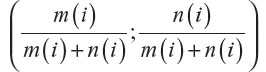after each (ith) arrival, with m(i) equal to the number of patients allocated to the first group after the ith arrival and n(i) equal to the number of patients allocated to the second group after the ith arrival; i=1, 2, 3, …, (m + n), where m and n are the two arms’ final sizes.

The two last columns of Table 1 shows the allocation results based on two different situations: intentional sequential allocation (ISA) developed by Fossaluza et al,¹² in which every new patient is allocated as it arrives and there is no information about the next patients in line; or optimal global allocation (OGA), which means the whole sample is known a priori and the optimal allocation for the final sample can be calculated by purposely dividing patients in the same stratum. In our case, the OGA method is the equivalent of minimization procedures. To obtain OGA results, we chose to divide each cell of the Table 2 and allocate half of the patients to each arm. If the number in the cell is odd, one of the patients will be allocated at the end together with the remaining of the other cells. The allocation of the remaining individuals of odd cells can be performed using (or not) randomization. In addition, once the two groups are divided and carefully balanced, the whole group can be randomly assigned to one of two treatments.

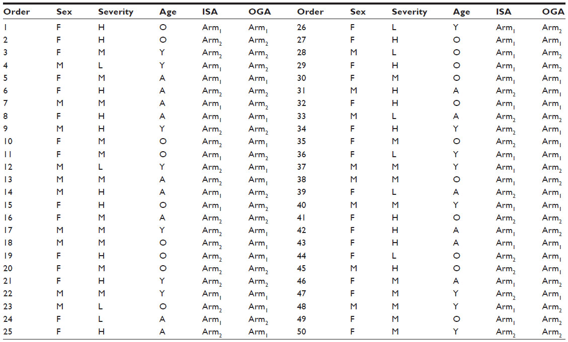Table 1 Results of two different allocation procedures for 50 patients with known parameters for sex, age, and initial severity Abbreviations: A, adult; F, female; H, high (severity); ISA, intentional sequential allocation; L, low; M, male (sex); M, medium; O, old; OGA, optimal global allocation; Y, young.

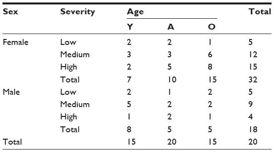Table 2 Contingency table with the observed frequencies of prognostic factors for 50 patients Abbreviations: A, adult; O, old; Y, young.

With the observed arrival sequential order in this experiment, we obtained the smallest possible distance between arms (0.0759) with both ISA and OGA procedures. Of note, although with equal distances, the results of allocation were not identical for ISA and OGA as shown in Table 3. Different orders of arrival, however, can produce suboptimal results for ISA in comparison with OGA. OGA represents the best allocation possible once the whole sample characteristics are known. ISA also aims optimality and it does not require that the whole sample is known beforehand. Therefore, ISA is a way to reach the best allocations possible in clinical trials that recruit and allocate patients sequentially with no prior knowledge of the next patients to be included.

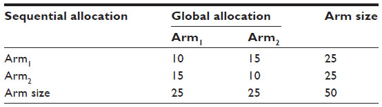Table 3 Contingency table that shows the difference between allocation results obtained with intentional sequential allocation and optimal global allocation

At this point, we will introduce a digression and quote the Indian statistician Debabrata Basu⁴:

The choice of a purposive plan will make a scientist vulnerable to all kinds of open and veiled criticisms. A way out of the dilemma is to make the plan very purposive, but to leave a tiny bit of randomization in the plan.⁴

As suggested by Basu, in the method described in Section 3, a tiny bit of randomization may be kept in the process of intentional allocation when no information is available or useful. There is as well another reason for just a bit randomization. In the situation in which (after several rounds of stratification) there is absolute equipoise in two groups, the allocation of remaining patients might be again randomized within their final joint stratum: such remaining patients (if any) are absolutely comparable with respect to every prognostic variable that the physician thought of. In other words, there is no information on prognostic factors that might be helpful to improve the balance of allocation. Furthermore, the effect of relevant differences that were not envisaged by the physician will be not his responsibility, and will be subjected to randomization (as they would anyway in a simple randomization procedure).

In the field of clinical trials, the hypothetical situation of total absence of useful information agreeable to all parts is unrealistic. Even in the total absence of prognostic information, at least baseline characteristics such as sex and age can be used for determining allocation as they might be associated with other variables of unknown and undisputed prognostic value. Even so, random decisions are kept in the process of intentional allocation after equipoise is attained.

To test Basu’s recommendation of pouring a little randomization, we calculated the effects of mixing up intentional allocation with simple randomization. We considered a mixture of the distance obtained with intentional allocation and the distance obtained if the allocation were defined by randomization: for a chosen small real number, ε, in the closed unit interval, the weighted average of the two distances, with weights (1–ε and ε), respectively. When ε equals 0, the allocation is completely intentional; when ε equals 0.1, the allocation is 90% intentional and 10% random; and so forth up to ε=1, which represents total randomization.

To compare procedures, we generated by simple simulation up to 50,000 ordered sequences of arrivals of the 50 patients in the current trial. There are N factorial (N! =N×(N−1)×… ×3×2=3.04×10⁶⁴) possible arrival orders with N patients enrolled in the trial, this being the reason we considered a simulation of 50,000 of them for the construction of Figures 2 and 3. To each of these sequences, we performed allocations using the following eleven values of ε, 0.00; 0.10; …; 0.90; 1.00.

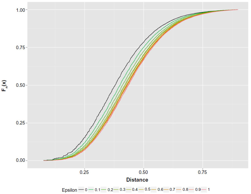Figure 2 Empirical distribution functions of the distances yield by the 50,000 simulated order arrivals for each of eleven epsilons.

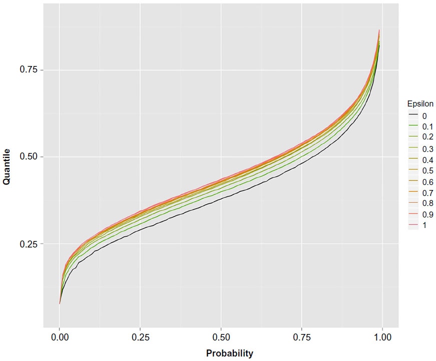Figure 3 Epsilon curves of the distance quantiles for their P-levels. Note: The x coordinate, abscissa, is the level of the quantile and the y coordinate, ordinate, is the value of the quantile.

Calculation particulars are fully explained by Fossaluza et al.^12,21 Simulations were fixed in up to 50,000 samples; however, to be fair in our comparison, we did not consider the simulated observations with less than 20 patients in one arm. Figures 2 and 3 illustrate up to 50,000 final distances distributions and quantiles that resulted from each value of ε.

For fixed values of ε, Figure 2 shows the empirical distribution functions of distances relative to up to 50,000 simulated orders of patient-arrival, illustrating the spread due to uncertainty that occurs. The highest curve is for ISA and the lowest is for full randomized allocation. Hence, ISA curve favors the smallest distance values when compared with all other curves. On the other hand, full randomization is the one that most favors higher distance values.

Figure 3 shows quantile curves of which ISA is the lowest and full randomization (ε=1) is highest. In other words, for all distance quantiles considered, ISA favors smaller values and again full randomization favors higher distance values. In other words, high differences between groups regarding predetermined factors are less likely with ISA than with random allocation.

The results illustrated in Figures 2 and 3 indicate that regarding uncertainty and balanced index (values of the distances), the optimal value of ε is zero and, therefore, no bit of randomization improves ISA. We also estimated the proportion of times ISA has performed better than any other mixing of randomization and ISA; ε=0.1;…;0.9;1. These results are described in Table 4. ISA performs better than any degree of randomization. As expected, ISA superiority is more evident when compared with the highest degrees of randomization (ε=1). The estimate 0.61 means that for 61% of the orders of arrival, ISA produced distances smaller than full random allocation.

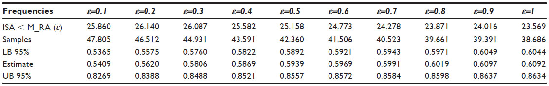Table 4 Proportions of cases in which intentional allocation performed better than randomized mixed with ISA Notes: LB 95% and UB 95% are the lower bound and upper bound of intervals with 95% of credibility. Abbreviations: ISA, intentional sequential allocation; M_RA, mixed intentional and random allocation.

Conclusion

In this article, we reviewed the reasons why researchers may withhold the implementation of methods of intentional allocation in clinical trials and evaluated the performance of a protocol for intentional allocation. We concluded that arguments in favor of randomization cannot be sustained in the face of the advantages of intentional allocation. In addition, the tested protocol of allocation achieved perfect or almost perfect joint balance of prognostic factors among treatment groups and their consequent comparability. It performed better than randomization in guaranteeing that unbalanced samples are not chosen. Using intentional allocation, it becomes less likely that the results of a study will be considered inconclusive due to the effect of a confounding factor, which is unbalanced between interventional groups. Therefore, the use of carefully designed methods of intentional allocation should be encouraged in future clinical trials.

Recommended reading

The effect of randomization in Medical Ethics has been described by Wajsbrot,²² Ware and Epstein,²³ Worral,²⁴ and Berry.²⁵ The conflict of ideas between advocates for randomization against intentional allocations is very old in the culture of statistics. It is hard to know where and when this methodological conflict started. We recommend the reading of some fundamental works of great scholars, such as Fisher,²⁶ Kempthorne²⁷ from the side of randomization, and Basu⁴ and Lindley²⁸ from the opposite viewpoint. The complete works of Fisher and Basu can be found in Fisher,²⁹ DasGupta,⁸ and Basu.³⁰

An important paper by Bruhn and McKenzie³¹ compares the power of balanced and random designs using methods pioneered by Student^32,33 and Pearson.³⁴ Curiously, Bruhn and McKenzie cite Fisher but not Student or Pearson.

Recent works attempting a compromise between randomization and purposive sampling are Pfeffermann³⁵ and Pfeffermann and Sverchkov.³⁶ In these two papers, purposive sampling is used just to incorporate available information (which is formally unadvised in frequentist statistical inference). Fossaluza et al²¹ make operational the introduction of Basu’s “bit of randomization”. There are certainly other fields in which purposive sampling is helpful: in robustness for instance, see Pereira and Rodrigues³⁷ under a frequentist perspective and the Bayesian counterpart is introduced by Bolfarine et al.³⁸ Finally, we recommend some sound foundational and formal work by Berry and Kadane⁷ and DeGroot.³⁹

Acknowledgments

The authors would like to thank Professor J Stern, an unabashed randomizer, for most insightful discussions. The Brazilian scientific agencies, CNPq, CAPES, and FAPESP, have been supporting the authors along the years (Grant numbers: CNPq, 304025/2013-5 and 458048/2013-5; CAPES, PNPD-2233/2009; FAPESP, 2013/26398-0, 2011/21357-9).

Disclosure

The authors declare no conflicts of interest in this work.

---

References

1.	Suresh K. An overview of randomization techniques: an unbiased assessment of outcome in clinical research. J Hum Reprod Sci. 2011;4(1):8–11.
2.	Struchiner CJ, Halloran ME. Randomization and baseline transmission in vaccine field trials. Epidemiol Infect. 2007;135(2):181–194.
3.	Basu D. An essay on the logical foundations of survey sampling survey, with discussions. In: Godambe VaS, DA, editor. Foundations of Statistical Inference. Toronto: Holt, Rinehart and Winston of Canada; 1971:203–242.
4.	Basu D. On the relevance of randomization in data analysis, with discussion. In: Namboodiri N, editor. Survey Sampling and Measurements. New York: Academic Press; 1978:267–339.
5.	Basu D. Randomization analysis of experimental data: the Fisher randomization test. J Am Stat Assoc. 1980;75:575–595.
6.	Brewer K. Combined Survey Sampling Inference: Weighing Basu’s Elephants. London: Hodder Arnold; 2002.
7.	Berry S, Kadane J. Optimal Bayesian randomization. J R Stat Soc Series B Stat Methodol. 1997;59:813–819.
8.	DasGupta A, editor. Selected Works of Debabrata Basu. New York, NY. Springer-Verlag New York; 2011.
9.	Kadane J, Seidenfeld T. Randomization in a Bayesian perspective. J Stat Plan Inference. 1990;25:329–345.
10.	Ware J. Investigating therapies of potentially great benefit: ECMO (with discussion). Statist Sci. 1989;4:298–306.
11.	Scott NW, McPherson GC, Ramsay CR, Campbell MK. The method of minimization for allocation to clinical trials: a review. Control Clin Trials. 2002;23:662–674.
12.	Fossaluza V, Diniz J, Pereira BB, Miguel E, Pereira C. Sequential allocation to balance prognostic factors in a psychiatric clinical trial. Clinics (Sao Paulo). 2009;64(6):511–518.
13.	Berry DA, Eick SG. Adaptive assignment versus balanced randomization in clinical trials: a decision analysis. Stat Med. 1995;14(3):231–246.
14.	Morgan K, Rubin D. Rerandomization to balance tiers of covariates. J Am Stat Assoc. 2015;110:1412–1421.
15.	McPherson GC, Campbell MK, Elbourne DR. Investigating the relationship between predictability and imbalance in minimisation: a simulation study. Trials. 2013;14:86.
16.	Berry D. Interim analysis in clinical trials: the role of the likelihood principle. Am Stat. 1987;41(2):117–122.
17.	Aitchison J. Principal component analysis of compositional data. Biometrika. 1983;70(1):57–65.
18.	Belotto-Silva C, Diniz JB, Malavazzi DM, et al. Group cognitive-behavioral therapy versus selective serotonin reuptake inhibitors for obsessive-compulsive disorder: a practical clinical trial. J Anxiety Disord. 2011;26(1):25–31.
19.	Diniz JB, Shavitt RG, Fossaluza V, Koran L, de Braganca Pereira CA, Miguel EC. A double-blind, randomized, controlled trial of fluoxetine plus quetiapine or clomipramine versus fluoxetine plus placebo for obsessive-compulsive disorder. J Clin Psychopharmacol. 2011;31(6):763–768.
20.	Aitchison J. The Statistical Analysis of Compositional Data. Caldwell: The Blackburn Press; 2003.
21.	Fossaluza V, Lauretto M, Pereira C, Stern J. Combining optimization and randomization approaches for the design of clinical trials. In: Polpo de Campos A, Neto FL, Ramos Rifo L, Stern JM, editors. Interdisciplinary Bayesian Statistics. Vol 118. New York: Springer; 2015:173–184.
22.	Wajsbrot D. Randomization and Medical Ethics (In Portuguese). São Paulo, SP: Mathematics and Statistics, University of São Paulo; 1997.
23.	Ware JH, Epstein MF. Extracorporeal circulation in neonatal respiratory failure: a prospective randomized study. Pediatrics. 1985;76(5):849–851.
24.	Worral J. Why there’s no cause to randomize. Br J Philos Sci. 2007;58:451–488.
25.	Berry D. Investigating therapies of potentially great benefit: ECMO: comment: ethics and ECMO. Statist Sci. 1989;4(4):306–310.
26.	Fisher R. The Design of Experiments. 2nd ed. Edinburgh: Oliver and Boyd; 1960.
27.	Kempthorne O. Why randomize? J Stat Plan Inference. 1977;1:1–25.
28.	Lindley D. The role of randomization in inference. The Philosophy of Science Association. Chicago: The University of Chicago Press; 1982.
29.	Fisher R. The Collected Papers of R. A. Fisher. Vol 1–5. Adelaide: University of Adelaide; 1971–1974.
30.	Basu D. Statistical Information and Likelihood. Ghosh JK, editor. New York, NY. Springer-Verlag New York; 1980.
31.	Bruhn M, McKenzie D. In pursuit of balance: randomization in practice in development economics. Am Econ J: Appl Econ. 2009;1:200–232.
32.	Student. On testing varieties of cereals. Biometrika. 1923;15:271–293.
33.	Student. Comparison between balanced and random arrangements of field plots. Biometrika. 1938;29:363–378.
34.	Pearson E. Some aspects of the problem of randomization: II. An illustration of Student’s inquiry into the effect of ‘balancing’ in agricultural experiment. Biometrika. 1938;30:159–179.
35.	Pfeffermann D. Modeling of complex survey data: why is it a problem? How should we approach it? Surv Methodol. 2011;37(2):115–136.
36.	Pfeffermann D, Sverchkov M. Fitting generalized linear models under informative sampling. In: Skinner C, Chambers R, editors. Analysis of Survey Data. New York: Wiley; 2003:175–195.
37.	Pereira C, Rodrigues J. Robust linear prediction in finite populations. Int Stat Rev. 1983;51(3):293–300.
38.	Bolfarine H, Pereira C, Rodrigues J. Robust linear prediction in finite populations: a Bayesian perspective. Indian J Statist. 1987;49(1):23–35.
39.	DeGroot M. Optimal Statistical Decisions. New York: McGraw-Hill; 1970.
40.	wikimedia.org [webpage on the Internet]. Astragalus monument. Arthoum; 2014. Available from: https://commons.wikimedia.org/w/index.php?curid=33740485. Accessed March 29, 2016.

---

Supplementary materials

Mathematics of randomization irrelevance

Ed and Joe had 924 different possible allocations of six patients to each group to choose from. In general, 2n patients can be allocated in (2n)!÷(n!)² different ways to two groups of n patients each for which n! being the well-known factorial of n. And there are (N!)÷[(n!)(N−n)!] different samples of size n, which can be extracted from a population of N patients. Each allocation (or each sample) has a numerical “value”, which can be thought of as the amount of information it will bring about the population (or about the effects of interventions). Such values depend also on the population (and the effects of interventions on its elements), which is of course unknown. These values can be ordered according to their averages taken over all population possibilities weighted by respective probabilities. This expected utility of each sample is therefore a real number that depends on the probability distribution (opinion) over the population and relative values (preference).

Mathematically, the choice of the sample that maximizes expected utility is implied by fundamental “rationality” axioms of opinion and preference. This is the so-called Maximization of Expected Utility Paradigm.

A randomized sample is always a convex combination of two or more nonrandom (or rigid or extreme) samples, in the sense that it ends up being one of the rigid samples with respective (randomization) probabilities. The following theorem formalizes the irrelevance of randomized samples (and allocations or choices in general) also in Mathematical Decision Theory (see DeGroot¹). Here, we write E[.] for expectation of the random element between brackets.

Theorem: Let Δ be a nonempty set (of choices), Θ a set of all possible population profiles, and U a utility function which assigns a nonnegative number to each pair (δ,θ). Consider a randomization which selects δ with probability π or δ₂ with probability (1−π) and let the resulting choice be represented by δ*. Then E[U(δ*)] is not larger than both expected utilities E[U(δ₁)] and E[U(δ₂)], for any 0 ≤ π ≤ 1, any δ₁, δ₂ in Δ, and any probability distribution over Θ.

Proof: The theorem of Total Probability implies:

and as π belongs to (0,1), we obtain, without loss of generality (due to assuming the inequality E[U(δ₁)] ≤ E[U(δ₂)]), the following result:

Aitchison distance for compositional data

Aitchison² presents the statistical analysis for compositional data. Here, we only describe the comparison of two samples respecting their vectors of frequency for a specific categorical variable and extend it to our particular case of four prognostic factors: severity, sex, age, and sample size.

Let the two arms k-vectors of compositional frequencies (with the addition of ½) of a prognostic factor for the two arms of a clinical trial. Each position of the vectors corresponds to a possible factor classification of the patients. Define the following functions:

For j=1, 2,…,k, k>0 being the number of possible classifications of the prognostic factor being evaluated, consider

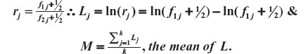
The Aitchison compositional distance between A₁ and A₂ is the standard deviation of L, that is,

As in our example we have four prognostic factors, we have four distances to be composed: severity, sex, age, and sample size. Let us represent the four distances as D_sev, D_sex, D_age, and D_sam. As the weights representing the importance of each factor, our overall distance is given by:

Recall that D_sam upon any new arrival t is given by:

Finally, we call attention to the fact that we had added ½ to all elements of the vectors involved to avoid the problem of zero frequencies.

References

---

1.	DeGroot M. Optimal Statistical Decisions. New York: McGraw-Hill; 1970.
2.	Aitchison J. Principal component analysis of compositional data. Biometrika. 1983;70(1):57–65.