Optic cup segmentation: type-II fuzzy thresholding approach and blood vessel extraction

Introduction

The optic nerve head (ONH) is where the retinal nerve fibers (axons of retinal ganglia) leave the globe of the eye. The ONH serves as an entry and exit region into the eye for the central retinal artery and the central retinal vein that provide nourishment for the retina. The ONH has a center portion called a cup. The cup size is important in the diagnosis of glaucoma. The death of nerve fibers caused by an increase in the fluid pressure inside the eye intensifies excavation (cupping) of the optic cup (OC), damaging the optic nerve. Untreated glaucoma leads to permanent damage of the optic nerve and irreversible loss of vision. Glaucoma is the second cause of blindness around the world after cataract. Since OC size (cupping) is the main diagnostic factor for glaucoma, the cup to disk ratio (CDR) can be used as an early indicator of abnormality in ONH. A good critical review of the literature on glaucoma image processing is given by Almazroa et al.¹ Ingle and Mishra² introduced cup segmentation based on intensity gradient. A segmentation based on vessel kinks was developed by Damon et al³ to detect the cup using the patches within the ONH. Issac et al⁴ proposed an automatic threshold segmentation-based method for detecting OC using local features of the fundus image. Liu et al⁵ presented a cup segmentation technique where the threshold-initialization–based level set was processed. Then, the level set formulation was applied to the initial contour to segment the OC boundaries. Joshi et al⁶ proposed an algorithm to segment the cup using vessel bends and pallor information. Nayak et al⁷ presented cup segmentation based on morphologic operations and thresholding. Kavitha et al⁸ developed a cup segmentation method using component analysis and active contour.

In this study, we describe a fully automatic algorithm for cup boundaries segmentation of fundus images. The proposed algorithm is based on a cup thresholding using type-II Fuzzy method that uses multilevel thresholds from a fundus image for segmentation. This method is adaptive and invariant to the quality of the image, that is, the method impacted by the quality of the images, whereas good image intensity provides good segmentation results and vice versa. The variable threshold increases the accuracy of the segmentation.

We considered image intensity and vessel kinking when developing the new OC automatic segmentation algorithm and evaluated the algorithm using retinal fundus images for glaucoma analysis (RIGA) dataset.⁹ This along with the optic disk (OD) image segmentation proposed by Almazroa et al¹⁰ leads to a comprehensive methodology for diagnosis of glaucoma from retinal fundus images.

The study is organized as follows: the “Methodology” section describes the proposed methodology including localization of the region of interest (ROI) algorithm. Results are presented and discussed in the next section, which is followed by the “Conclusion” section.

Methodology

Localizing the ROI

In order to separate the ROI from the entire image, a localizing technique was applied. The technique was introduced by Burman et al¹¹ and used an interval type-II fuzzy entropy-based thresholding scheme along with differential evolution. This is a powerful metaheuristic technique for faster convergence and lower computational time complexity in order to determine OD location. The multilevel image segmentation technique segmented an image into various objects in order to find the brightest object, which was located in the OC, and hence a part of the OD. Instead of a single membership value as in type-I fuzzy technique, here a range of membership values were introduced. A measurement called ultra fuzziness was used to obtain image thresholds.¹¹ Two thresholds were applied after transferring the image to gray level in order to divide the image into three objects or backgrounds.

OC segmentation

Figure 1 shows the flowchart of the cup segmentation algorithm. The localized image was the starting point, that is, finding the ONH to process the algorithm instead of processing the entire image. The goal was to segment the cup boundaries, and four loops were used to achieve the best cup segmentation. The algorithm was built based on 200 training images from the RIGA dataset. Trial and error technique was used to reach the best results. After localizing the ONH, the image was enhanced by stretching the image contrast and equalizing the histogram to increase the variation among the image parts including the retina, rim, blood vessels and cup. This can be seen in the first column of Figure 2 for the original image and for only the first two loops. The blood vessels were extracted using a top-hat transform on the G-channel of the fundus image. The blood vessels have more contrast in the G-channel, making the top-hat transform suitable for extraction of the small vessels. Detecting the small vessel kinks led to detecting the cup boundaries, as can be seen in the second column of Figure 2. The blood vessels were thresholded using Otsu’s algorithm.¹² Top-hat transform basically is the difference between the original image and its opening operation. Otsu’s algorithm, however, is a clustering-based image thresholding algorithm which computes the best threshold value based on the assumption that the image has two classes of pixels (foreground and background). The blood vessel extracting operation was used to detect the curvature of blood vessels (kinks) which indicate the cup boundary. The blood vessels were removed, since they restricted the cup threshold intensity (Figure 2, third column). The thresholds were more accurate in the localized image than in the entire image; hence, the localized image was applied to find the OD in the preprocessing. The localized image is a small portion of the original image with very limited variation in contrast. There were clear variations among the retina, blood vessels, rim area and cup of the original image (Figure 2, first column). The four loops of the proposed algorithm are for four different threshold values based on some conditions. Three thresholds were applied as the first loop to create four parts or backgrounds. Increasing the threshold values worked very well with good-quality images; however, it did not provide better results for poor-quality images. In some cases, increasing the threshold value significantly increased the computation time and the results were still not satisfactory. Therefore, after trying threshold values of up to 30, we applied only three thresholds due to their effectiveness in terms of area and centroid, as compared with the manual marking in the training set. After applying the threshold, the cup was estimated as the brightest spot in the localized images. However, sometimes there were additional small bright spots. Therefore, the white spots smaller than 50 pixels were eliminated to reduce the error in approximating the cup. The blood vessels were brought back to fill the gaps in the white spots (Figure 2, fourth column). A morphologic closing operation was applied to close the small gaps that remained in the white spots even after adding the blood vessels. This approach prevents potential errors when applying Hough transform for cup detection.¹³ Applying two thresholds are considered as a second loop, as shown in the flowchart in Figure 1. Two conditions were considered in order to go to the second loop (Figure 1). These were: 1) if the cup size is <3,000 pixels and 2) if the cup size is >16,000 pixels. The disc size was estimated in order to increase the accuracy of the cup results and reduce the error. Therefore, the aforementioned 16,000 pixels were estimated as a disc size and particularly for the images with size of ≤2,400×1,600 pixels. While for images size ≥2,400×1,600 pixels, the two conditions were: 1) if the cup size is <3,000 pixels and 2) if the cup size is >25,000 pixels. The same conditions were considered for the third loop, while in this case, four thresholds were applied. However, unlike the first two loops, there was no image enhancement in the third loop. If the segmentation for the third loop matched the aforementioned two conditions, then the fourth loop was applied for three thresholds without image enhancement. For any loop, when the two conditions were not met, the cup area and centroid were calculated.

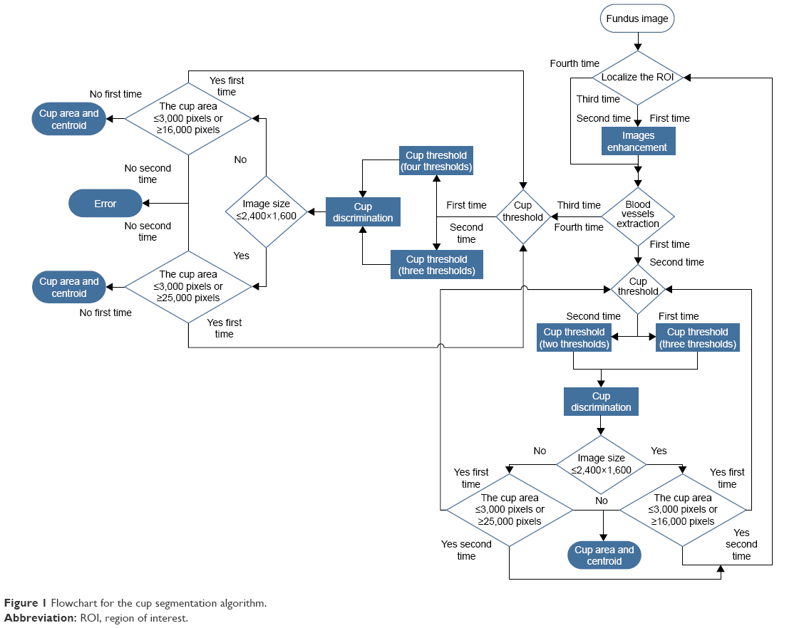Figure 1 Flowchart for the cup segmentation algorithm. Abbreviation: ROI, region of interest.

Figure 2 The cup segmentation procedures. Note: The first column from the left is the localized image from the original, the second column is the thresholded blood vessels, the third column is the thresholded cup, the fourth column is the second and third columns together and the fifth column is the algorithm results for the cup segmentation (blue circle).

Figure 2 shows the results of the algorithm for four different images with different cup situations. The image in the first row represents unclear cup intensity with clear blood vessel kinks; the image in the second row represents clear cup intensity with some blood vessel kinks; the image in the third row represents unclear cup intensity without any blood vessel kinks; and finally the image in the fourth row represents clear cup intensity with clear blood vessel kinks. The area calculations showed good results when compared with manual markings. The calculations of centroids did not give good results practically on the X axis due to the blood vessels specifically on the nasal side. The algorithm up to this point was tested on 100 images from MESSIDOR dataset and the results are shown in Almazroa et al.¹³ Therefore, a function was developed to include the blood vessels in the nasal side of the cup. The disk segmentation centroid was also involved to improve the cup centroid estimation.

The area inside the disk was considered a more localized image for solving the centroid problem only along the X axis. Three small squares of 25×25 pixels were created on the same centroid X axis of the segmented cup in order to measure the highest intensity of blood vessels among the three squares (Figure 3); the cup segmented border was then dragged inside the selected square. If the segmented image was on the right side, then the three squares would have been on the right half of the segmented disk and vice versa. Three options based on positions were considered inside the selected square: 1) the square near edge to the centroid of the segmented cup, 2) the middle of the square and 3) the square far away edge which was always close to the disk boundaries as shown in the second row of Figure 3A–D. The final decision for the cup position among the three positions was based on the disk centroid, that is, the cup went through all three positions and the one with the cup centroid closest to the disk centroid was chosen as the best X segmented cup centroid. This approach made the blood vessels on the nasal side 100% inside the boundary of the segmented cup, where the blood vessels always cover the cup boundaries in this area (nasal side). On the other hand, after choosing the best X axis, the Y axis was fixed so that the maximum distance between the disk and the cup Y axes was ≤10 pixels. This selection of 10 pixels was arbitrary. For example, if the difference between the disk (green dot) and the cup (blue dot) in Y axis was 12 pixels, the cup was automatically moved down 2 pixels (Figure 3A). In the first row of Figure 3A, the first panel represents the localized image, the second panel represents the thresholded cup with the extracted blood vessels, while the third panel is the segmented cup, which was the final step for the 100 images tested previously. In this image, the centroid results were not in agreement with the results of manual markings by the six ophthalmologists. The last panel in this row shows the results of the proposed algorithm. Here, the middle square has the most blood vessel pixels intensity; therefore, the nasal cup boundaries must be dragged inside it. As long as the boundaries are inside the square (as shown in the first image in the second row), the difference between the disk centroid and the cup centroid in the Y axis remains >10 pixels. Therefore, the cup was moved down until the difference between the two centroids was exactly 10 pixels. The second image shows the near edge adjustment with the new Y axis. The third image shows the middle edge adjustment which was the same as the original, while the last image is the far away adjustment. Based on the criteria, the best decision matching the six ophthalmologists’ manual marking centroid results was the middle edge adjustment, which was the same as the original and the shortest distance between the disk centroid and the cup centroid. The same procedures were applied to the second image in Figure 3B. The middle square had the most blood vessel pixels intensity as shown in the last panel of the first row. For the Y axis, the distance between the disk centroid and the cup centroid was <10 pixels; therefore, there was no need to move the cup Y centroid. While for the X axis, the segmentation was tested for all the three adjustments in addition to the original position, as shown in the second row. The best decision made based on the shortest distance between the two centroids was far away adjustment as can be seen in the first image in the second row, and gave good results when compared with the six manual markings. The same was true for case (C) in which the best decision was the edge middle adjustment, and there was no need to change the Y axis. In the last case, that is, case D, there was no need for any change because the Y axis gave good results and in the X axis, the original segmentation gave the shortest distance between the two centroids. Finally, the segmented disk boundaries were considered now for the loops conditions rather than the number of pixels, which were 16,000 pixels for image sizes of ≤2,400×1,600 p and 25,000 pixels for larger images.

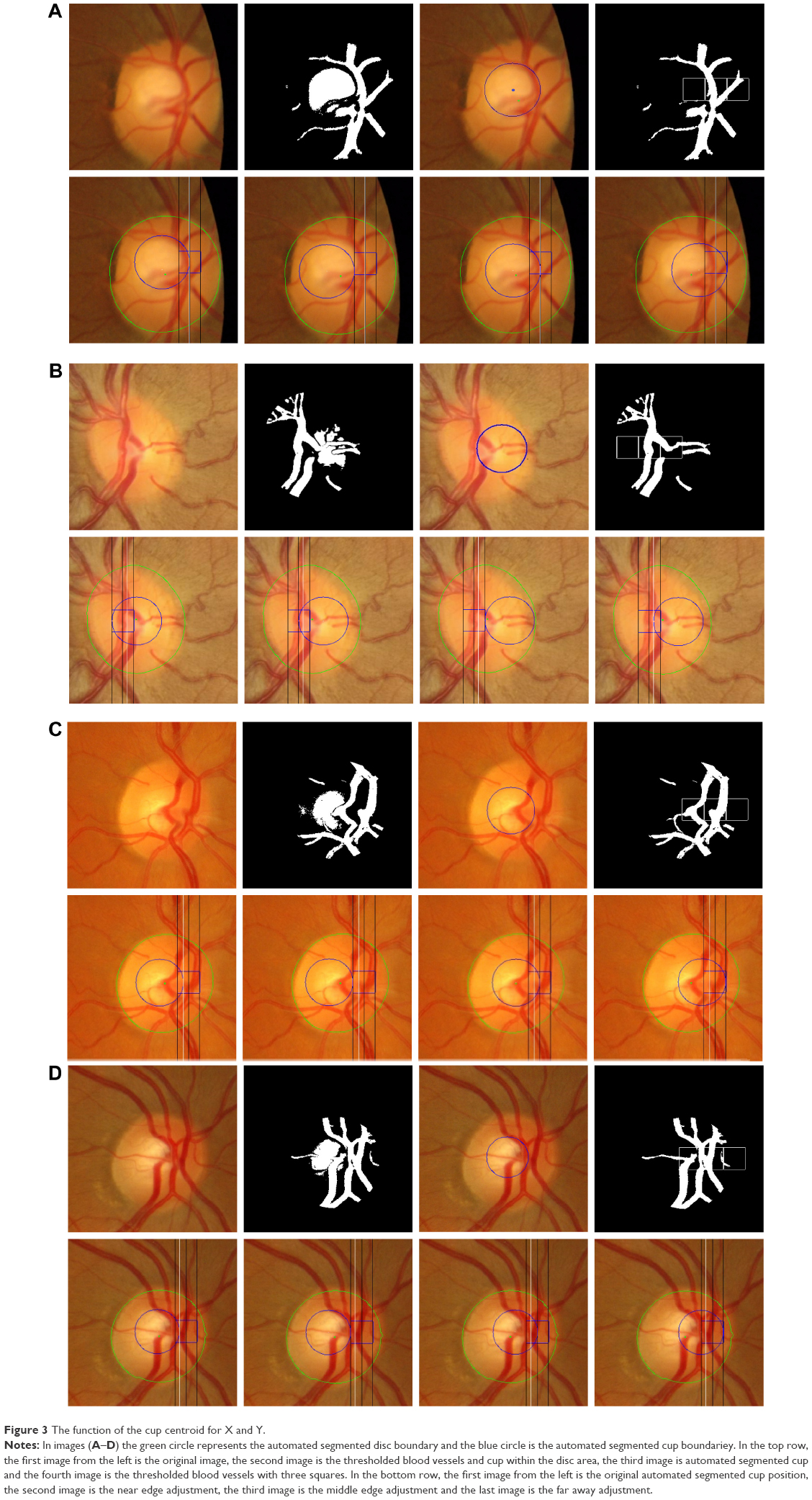Figure 3 The function of the cup centroid for X and Y. Notes: In images (A–D) the green circle represents the automated segmented disc boundary and the blue circle is the automated segmented cup boundariey. In the top row, the first image from the left is the original image, the second image is the thresholded blood vessels and cup within the disc area, the third image is automated segmented cup and the fourth image is the thresholded blood vessels with three squares. In the bottom row, the first image from the left is the original automated segmented cup position, the second image is the near edge adjustment, the third image is the middle edge adjustment and the last image is the far away adjustment.

Results

Cup results

The simulation was performed in Matlab 2014b environment in a workstation with Intel Core i-7 2.50 GHz processor. Figure 4 shows the flowchart for analysis of cup segmentation.

Figure 4 Flowchart for analysis of cup segmentation. Abbreviation: SD, standard deviation.

Figure 5 compares the results of automatic segmentation and the manual markings by six ophthalmologists. The first column shows the manual marking by ophthalmologist number one, the second column shows the manual marking by ophthalmologist number two, and so on. The seventh column represents the result of automatic segmentation. The four rows represent four different images with different situations. In the first row, the markings by all six ophthalmologists were close to each other in terms of area and centroid and the algorithm gave the same results. In the second row, the manual marking of area size by ophthalmologist number five was an outlier and was eliminated from the analysis. In this row, the results of the algorithm were in good agreement with the markings by the other five ophthalmologists. For the first three images, the algorithm gave perfect results in terms of area and centroid. In the last image, the manual marking of centroid by ophthalmologists two and six were outliers, that is, if an image has a standard deviation (SD) greater than the mean SD for area or centroid, this implies the ophthalmologist has created an outlier by annotating either a very small or a very large area as the OC area or either far left, right, up or down in terms of centroid. Therefore, the two images were eliminated. In the same image, the manual markings of area by ophthalmologists three and five were outliers, thus they were eliminated too. As a result, four images were removed. Here, there was no agreement among the markings done by the ophthalmologists, and therefore, this image was not considered in evaluation of the algorithm. The automatic algorithm produced results similar to the markings by two ophthalmologists.

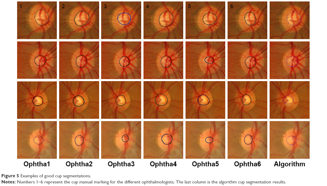Figure 5 Examples of good cup segmentations. Notes: Numbers 1–6 represent the cup manual marking for the different ophthalmologists. The last column is the algorithm cup segmentation results.

Figure 6 shows examples of poor cup segmentations. The six ophthalmologists’ manual markings of cup are shown in the first six columns from left, starting from ophtha1 to 6. The far right column shows the result of automatic cup segmentation. In terms of area and centroid, there was agreement in markings of the first image among all six ophthalmologists, while the algorithm gave a much bigger cup area that was accounted as an outlier. For the second image, cup area markings by ophthalmologists two and four were outliers and, therefore, were eliminated from the analysis. The algorithm also marked a small area as the cup area; this was also an outlier. As can be seen in the localized image, the right half of the retina has a bright intensity and this affected the cup thresholding. For the last case, only the manual marking by the fourth ophthalmologist was eliminated. The algorithm gave a small area and bad OC position (centroid). Also, in this case, the intensity of the retinal part was variable as well as the rim area (particularly the right side), which negatively affected the cup thresholding.

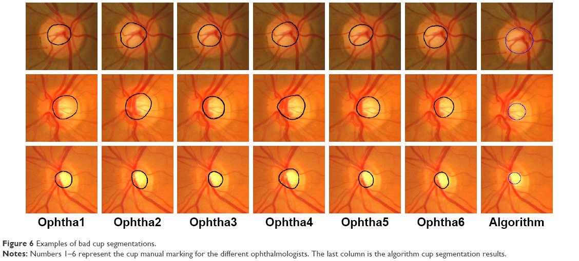Figure 6 Examples of bad cup segmentations. Notes: Numbers 1–6 represent the cup manual marking for the different ophthalmologists. The last column is the algorithm cup segmentation results.

Results of Bin Rushed dataset

Table 1 shows the cup segmentation with details for Bin Rushed dataset, the first image resource of RIGA dataset, which includes 195 images. The ONH was not localized in ten images; therefore, they were eliminated. For the cup area, only one image with the mean SD between the six ophthalmologists >2,150 pixels was eliminated.¹⁴ In total, 184 images were tested. The cup area was successfully segmented in 152 images (82.6%).

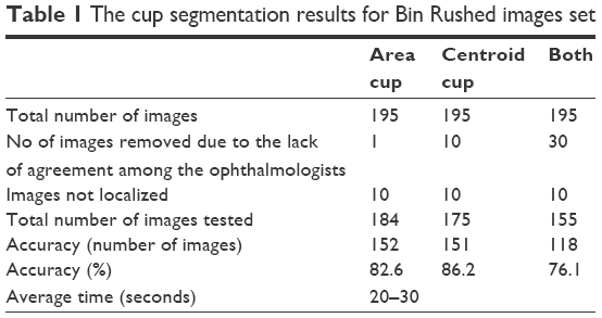Table 1 The cup segmentation results for Bin Rushed images set

For the cup centroid, there were ten images for which the markings by more than three ophthalmologists were considered outliers; therefore, these images were eliminated from further analyses. In total, 175 images were tested for cup centroid, and the cup was successfully segmented in 151 images (86.2%). For both area and centroid, 30 images with either poor area marking or poor centroid marking were eliminated. Therefore, in total, 155 images were tested and 118 images were successfully segmented in terms of area and centroid (76.1%). The average time to run the algorithm was between 20 and 30 seconds.

To further evaluate the result of automatic segmentation, its accuracy was compared with the accuracy of the markings by the six ophthalmologists (Table 2). Similar to the analysis of OD, the performance of each ophthalmologist was evaluated based on its agreement with the performance of the other five ophthalmologists. An image was eliminated if at least three ophthalmologists did not agree with each other in markings of area or centroid. If for an image the markings by two ophthalmologists were outliers for area, and the marking by a third ophthalmologist was an outlier for centroid, then the image was removed.¹⁴ Twenty-four images marked by ophthalmologist number one were removed from the evaluation due to lack of agreement with markings by other ophthalmologists. In total, 161 images were tested and the accuracy was 143 images (88.8%). For ophthalmologist number two, markings of 16 images did not agree with markings by others; therefore, these images were removed from further analysis. In total, 169 images were tested and the accuracy was 139 images (82.2%). For ophthalmologist number three, 21 images were removed; therefore, in total, 164 images were tested and the accuracy was 134 images (81.7%). In total, 173 images were tested for ophthalmologist number four and the accuracy was only 85 images (49.1%), mostly this ophthalmologist annotating the cup largely comparing with the other five. The total number of images tested for ophthalmologist number five was 165 images and the accuracy was 136 images (82.4%). Finally, the total number of tested images for ophthalmologist number six was 165 images and the accuracy was 133 images (80.6%). Twelve to 24 images were eliminated from each analysis.

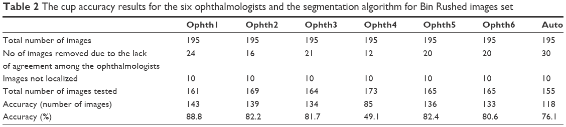Table 2 The cup accuracy results for the six ophthalmologists and the segmentation algorithm for Bin Rushed images set

While the performance of each ophthalmologist was compared with that of the other five ophthalmologists, the algorithm’s results were compared with the markings by all six ophthalmologists.¹⁴ Nevertheless, the algorithm’s cup segmentation accuracy was within the same range and was close to accuracy of the markings by ophthalmologists two, three, five and six.

Results of Magrabi dataset

Table 3 shows the results for the second image resource, that is, Magrabi dataset. As presented in Almazroa et al,^9,14 Magrabi dataset includes large images. The mean SD for the cup area as marked by the ophthalmologists was 8,800 pixels, whereas the mean SD for the cup centroid was 11 pixels. The mean SD for area and centroid among the six ophthalmologists was more accurate in this image set than the other two sets due to image sizes as well as the fact that the images had been captured by mydriatic fundus camera and, therefore, were clearer and easier to manually mark. Ten images were excluded: four due to lack of agreement among the ophthalmologists and six images because they could not be localized. Therefore, in total, 85 images were tested. The algorithm’s segmentation accuracy was 70 images or 82.3%. Eleven images were eliminated due to disagreement among the ophthalmologists for the cup centroid. Therefore, in total, 78 images were tested and the algorithm’s segmentation accuracy was 63% or 80.7%. Twenty images were removed when testing for both area and centroid; therefore, in total, 50 images (72.4%) were tested, which was less than the percentage of images tested from Bin Rushed dataset. The average time to run the algorithm was between 70 and 120 seconds due to the size of images, which increased the time required to achieve the level set approach used to improve the cup centroid.

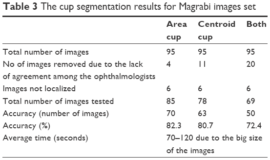Table 3 The cup segmentation results for Magrabi images set

The cup segmentation accuracy (Table 4) was close to the accuracy of markings by ophthalmologists three and four. Twenty images were removed due to disagreement among the six ophthalmologists. Therefore, the accuracy of algorithm might have suffered due to the fact that fewer images were used to test the algorithm.

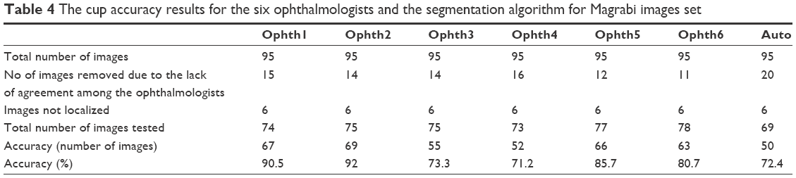Table 4 The cup accuracy results for the six ophthalmologists and the segmentation algorithm for Magrabi images set

Results of MESSIDOR dataset

The results of MESSIDOR dataset are shown in Table 5. The high number of images in this dataset and their good quality resulted in more accurate results; indeed, the accuracy of markings using this dataset was higher than the accuracy of markings using the other two datasets. Similar to Bin Rushed dataset, ten images from MESSIDOR dataset were not localized. Five images were eliminated from calculation of the area. In total, 245 images were tested and the accuracy was 206 images (84%). A higher percentage of accuracy was obtained for calculation of centroid. Twelve images were eliminated from calculation of centroid. Therefore, in total, 238 images were tested for centroid and the accuracy was 216 images (90.7%). Thirty-three images were removed from evaluation of both area and centroid. In total, 217 images were tested and the accuracy was 177 images (81.5%). The average running time for the algorithm was between 20 and 30 seconds, which was similar to the time required for running the algorithm for Bin Rushed dataset, and this was due to their similarity in size.

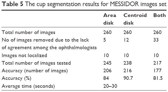Table 5 The cup segmentation results for MESSIDOR images set

The percentage accuracy of markings by the six ophthalmologists was 86%–89%, while the algorithm’s accuracy was 81.5%. The algorithm was tested on a total of 177 images, while 195–203 images were used to test the accuracy of manual markings by all ophthalmologists except for ophthalmologist number four (Table 6). As mentioned previously, increasing the number of test images boosts the accuracy. The algorithm shows good accuracy, especially when compared with the accuracy of markings by ophthalmologists one, two and six.

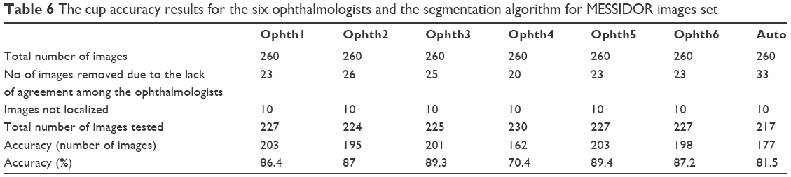Table 6 The cup accuracy results for the six ophthalmologists and the segmentation algorithm for MESSIDOR images set

Consolidated results

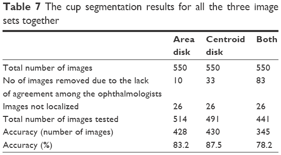
In this section, all images are gathered in order to have a comprehensive analysis between the markings by the ophthalmologists and algorithm. Exactly 550 images from all three datasets were tested to evaluate the algorithm and the six manual markings. If an image had three outliers or more in the area or centroid or both, it was considered a bad image and was removed from the corresponding analysis. From the three datasets, ten images were eliminated from cup area analysis due to disagreement among ophthalmologists. Also, 26 images were eliminated due to bad localization. Therefore, in total, 514 images were tested and the accuracy was 428 images or 83.2% (Table 7). On the other hand, 33 images were removed from the analysis of cup centroid due to disagreement and 26 images due to localization. Therefore, in total, 491 images were tested and the accuracy was 430 images or 87.5%. This result was better than the result of area analysis; however, the number of images accurately marked was very similar for the cup area and centroid, that is, 428 versus 430 images for area and centroid, respectively. Therefore, the number of images with disagreement in centroid was advantageous and increased the accuracy. Eighty-three images were eliminated from analysis of both area and centroid, in addition to 26 images that were not localized. Therefore, in total, 441 images were tested and the accuracy was 345 images or 78.2%. This was obviously due to the fact that there were many images with good accuracy in terms of area that were outliers in terms of centroid and vice versa.

Table 7 The cup segmentation results for all the three image sets together

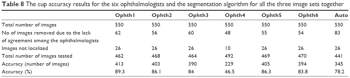
Ophthalmologist number one had the best accuracy in comparison with the other five ophthalmologists (Table 8), even though his manual marking had been tested using only 462 images, the lowest number of images among all ophthalmologists. The algorithm had been tested using 441 images and the accuracy was 345 images (78.2%). The performance of the algorithm in terms of percentage accuracy in cup segmentation was close to that of ophthalmologist number six, then ophthalmologist three, then ophthalmologist two, and finally ophthalmologist five.

Table 8 The cup accuracy results for the six ophthalmologists and the segmentation algorithm for all the three image sets together

Figure 7 shows the results of markings by all six ophthalmologists as well as the automatic algorithm for all three datasets. The blue line represents Bin Rushed dataset, the dark orange line represents Magrabi and the gray line represents MESSIDOR images, while the bright orange line represents all images together. As can be seen in the figure, ophthalmologists one, five and six and the algorithm showed similar performance in terms of accuracy of cup segmentation for all three datasets. Magrabi images were most accurately marked by ophthalmologists one, two and four. MESSIDOR images were most accurately marked by ophthalmologists three, five and six. Magrabi images gave low accuracy for ophthalmologists three and four as well as the algorithm. Overall, ophthalmologist number six had the closest results to the algorithm.

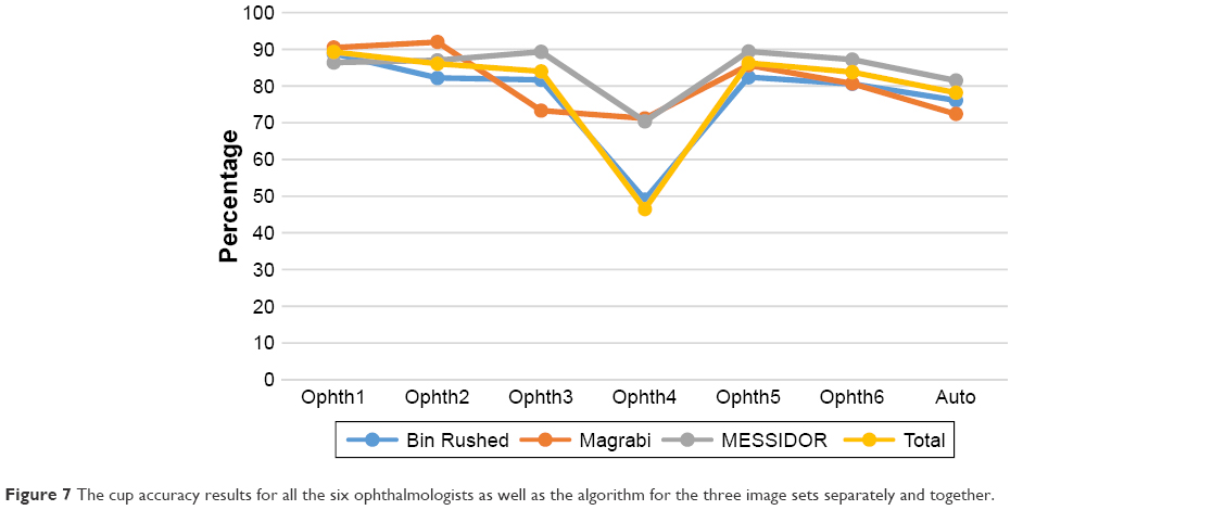Figure 7 The cup accuracy results for all the six ophthalmologists as well as the algorithm for the three image sets separately and together.

Agreement for the cup

In terms of cup area and centroid image agreement and similarity, the markings by all ophthalmologists had the best agreement with the markings by ophthalmologist number one (Table 9). The best agreement for the algorithm was with ophthalmologist number one in 359 images (65.2%), whereas the lowest agreement was with ophthalmologist number six in 329 images (59.8%). On the other hand, the best overall agreement was between ophthalmologist number one and ophthalmologists two and five in 398 images (72.3%) and the lowest agreement was between ophthalmologist number four and the algorithm. Variations of the overall agreement in markings of the disk were between 56.7% and 74.5%, which is also slightly better than the cup. Variations of the overall agreement in manual annotations of the disk were between 56.7% and 74.5%, which is also slightly better than the cup.¹⁰ The ranking order scale for agreements was almost similar to the ranking order scale for accuracy.

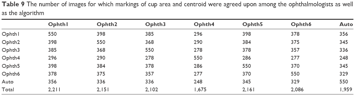Table 9 The number of images for which markings of cup area and centroid were agreed upon among the ophthalmologists as well as the algorithm

Figure 8 shows the agreement for every ophthalmologist in addition to the algorithm. The algorithm clearly had the best agreement with ophthalmologist number one, then ophthalmologist number five, then ophthalmologist two and three, then ophthalmologist number six and finally with ophthalmologist number four. The agreement was evaluated based on an accurate parameter. The number of pixels was considered to calculate the SD which is a small number; therefore, 1 pixel of thousands of pixels might be making the agreement. As a result, the number of agreement seems to be low.

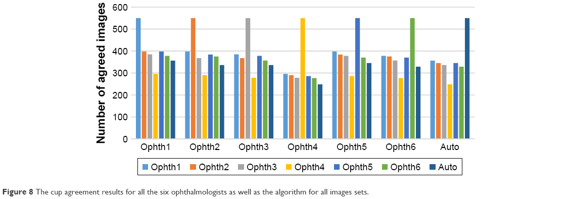Figure 8 The cup agreement results for all the six ophthalmologists as well as the algorithm for all images sets.

Figure 9 shows the total number of agreements for all ophthalmologists as well as the algorithm. Ophthalmologist number one is the best, then ophthalmologist number five, number two, number three, number six, the algorithm and finally ophthalmologist number four. Except for ophthalmologist number four and the algorithm which had close to 2,000 images, all other ophthalmologists had >2,000 images in total.

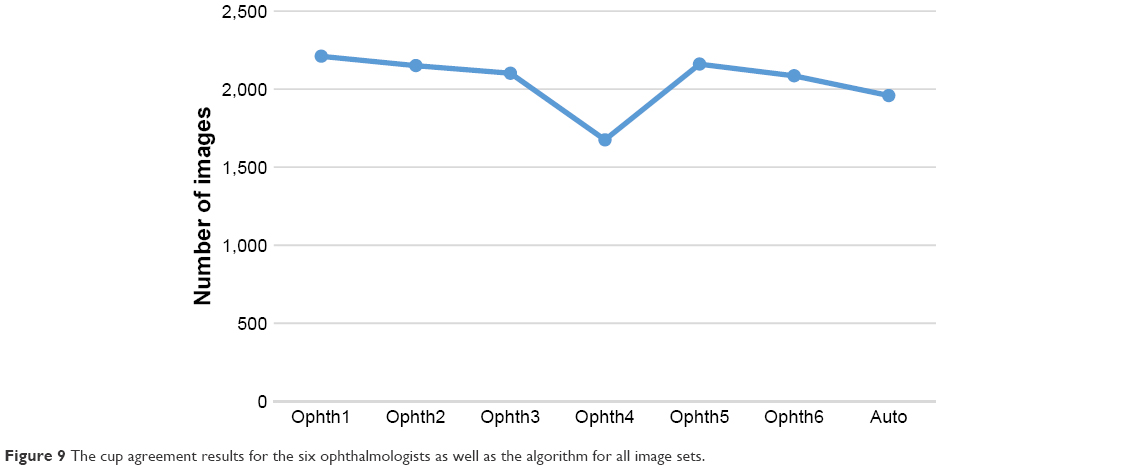Figure 9 The cup agreement results for the six ophthalmologists as well as the algorithm for all image sets.

Discussion

This study aimed to improve a previously presented¹³ OC segmentation algorithm. The OD segmentation algorithm we had introduced previously¹⁰ was used in the cup segmentation. The algorithm was used to include the blood vessels in the nasal side into the segmented cup and then solve the centroid problem. The centroid of the segmented disk was the reference for the centroid of the segmented cup. Three squares were created based on the cup centroid in the nasal side. From the three squares, the one with the highest intensity of segmented blood vessels was selected. The position of the segmented cup on the nasal side was tested on the selected square. The segmented cup was dragged into three positions relative to the square. These positions were in addition to the original position of the segmented cup without considering the square. The final cup centroid was based on the cup centroid position closest (among the four positions) to the disk centroid on the X axis. For the Y axis, the improvement was considered only the distance between the Y cup centroid axis in the final X position and the disk Y axis. The distance had to be no more than 10 pixels. The disk contour was also considered to have four loops for cup segmentation. These loops are: 1) three thresholds with image enhancement, 2) two thresholds with image enhancement, 3) four thresholds without image enhancement and 4) three thresholds without image enhancement. Any touch for the segmented cup contour to the disk contour was accounted as an error. The opinions of six ophthalmologists were considered to train and evaluate the algorithm. To increase the reliability of algorithm evaluation, RIGA dataset was filtered and images that were not agreed upon by at least four ophthalmologists were removed from the analysis. The algorithm results are close to the six ophthalmologists, except ophthalmologist four. The accuracy for any ophthalmologist was considering only the other five. Therefore, the tested images were more and this was impacting the accuracy results. In contrast, the accuracy of algorithm was based on the all six ophthalmologists. This led to a reduction of the number of images tested by the algorithm. Therefore, the accuracy was lower when compared to the six ophthalmologist’s results.

The algorithm requires further improvement. More functions need to be developed to take into account the tortuous the blood vessel kinks, especially the smaller ones. The disk contour could be used to improve cup segmentation accuracy with the blood vessels specifically on the nasal side. The blood vessels (kinks) extraction might be used with other cup segmentation techniques, and these issues need to be investigated. However, we have presented herein a robust algorithm for cup estimation. The algorithm results have been compared with manual markings by ophthalmologists on the same images. This together with the previous study on disk estimation will allow a quick estimate of the CDR, a major diagnosis metric.

In conclusion, the average of accuracy between the ophthalmologists except four and the algorithm is close. In this study, the variations between the ophthalmologists’ markings are pointed out, which was never done before as most of the previous investigations were based on one opinion, making the algorithm’s accuracy less. This algorithm is a part of a screening system for glaucoma by combining the disk algorithm with the cup algorithm in order to calculate the horizontal and vertical CDR.

Disclosure

The authors report no conflicts of interest in this work.

---

References

1.		Almazroa A, Burman R, Raahemifar K, Lakshminarayanan V. Optic disc and optic cup segmentation methodologies for glaucoma image detection: a survey. J Ophthalmol. 2015;2015:180972.
2.		Ingle R, Mishra P. Cup segmentation by gradient method for the assessment of glaucoma from retinal image. Int J Eng Trends Technol. 2013;4:(6)2540–2543.
3.		Damon WWK, Liu J, Meng TN, Fengshou Y, Yin WT. Automatic detection of the optic cup using vessel kinking in digital retinal fundus images. Proceedings of the 9th IEEE International Symposium on Biomedical Imaging (ISBI), Barcelona, Spain; 2012. 2012:1647–1650.
4.		Issac A, Sarathi M, Dutta M. An adaptive threshold based image processing technique for improved glaucoma detection and classification. Comput Methods Programs Biomed. 2015;122(2):229–244.
5.		Liu J, Wong DWK, Lim JH, Li H, Tan NM, Wong TY. ARGALI: an automatic cup-to-disc ratio measurement system for glaucoma analysis using level-set image processing. Proceedings of the 13th International Conference on Biomedical Engineering. Singapore; 2009. 2009;559–562.
6.		Joshi GD, Sivaswamy J, Krishnadas S. Optic disk and cup segmentation from monocular color retinal images for glaucoma assessment. IEEE Trans Med Imaging. 2011;30(6):1192–1205.
7.		Nayak J, Acharya UR, Bhat PS, Shetty N, Lim TC. Automated diagnosis of glaucoma using digital fundus images. J Med Syst. 2009;33(5):337–346.
8.		Kavitha S, Karthikeyan S, Duraiswamy K. Early detection of glaucoma in retinal images using cup to disc ratio. In Proc of the International Conference on Computing Communication and Networking Technologies (ICCCNT). 2010;1–5.
9.		Almazroa A, et al. RIGA: as database of retinal fundus images for glaucoma analysis. IEEE Trans Med Imaging. In press 2016.
10.		Almazroa A, Sun W, Alodhayb S, Raahemifar K, Lakshminarayanan V. Optic disc segmentation: level set methods and blood vessel in painting. Submitted for publication. IEEE Trans Med Imaging. 2016.
11.		Burman R, Almazroa A, Raahemifar K, Lakshminarayanan V. Automated detection of optic disc in fundus images. Adv Opt Sci Eng. 2015;327–334.
12.		Otsu N. A threshold selection method from gray-level histograms. Automatica. 1975;11:23–27.
13.		Almazroa A, Alodhayb S, Burman R, Sun W, Raahemifar K, Lakshminarayanan V. Optic cup segmentation based on extracting blood vessel kinks and cup thresholding using Type-II fuzzy approach. In Proc of the 2nd International Conference on Opto-Electronics and Applied Optics (IEM OPTRONIX). 2015;1–3.
14.		Almazroa A, Alodhayb S, Osman E, et al. Agreement among ophthalmologists in marking the optic disc and optic cup in fundus images. Int Ophthalmol. 2016:1–17.