New method for identifying abnormal milling states of an otological drill

Introduction

With improving living standards, the demand for better health care is growing. As a kind of necessary tool for doctors, medical apparatus and instruments are playing more and more important roles in therapeutic process. The development of modern medicine has required increasingly intelligent and automatic medical equipment, one type of which is surgical instruments. Over the past several decades, with developments in mechanics and electronics, surgical instruments have been continually improved, making many surgical procedures safer.

The otological drill is one of the fundamental tools used in ear surgery. It is usually used to mill holes in the skull to remove diseased tissue or provide access for further intervention, including cochlear implantation.¹ It is controlled directly by the operating surgeon, and requires a high degree of hand-foot coordination, with one hand controlling its path and one foot controlling its switch state. As an intracranial surgery of high risk, the surgical cavity for otological surgery is narrow (Figure 1). The drill bit, which operates at high speed, can easily damage important intracranial structures.²

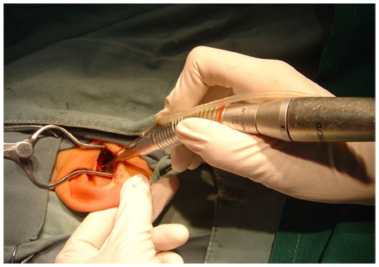Figure 1 Milling process in otological surgery.

Milling beyond the bone tissue wall is a common fault during the milling process.² In intracranial surgery, a hole in the bone has to be milled. When the bone is milled very thin, even the slightest touch may cause the high-speed rotating drill bit to break through the bone wall, causing unexpected damage to the patient’s tissues. Preventing the drill from penetrating the bone wall is a difficult task for surgeons.³ During a surgical procedure, surgeons have to estimate the thickness of the remaining bone covering the patient’s tissue.

Cotton swabs are used to stop bleeding at the surgical site. These swabs can easily become entangled with the rotating drill bit, and cause damage at the surgical site. It is also hard for surgeons to stop the entangled drill bit in a timely manner and avoid damage to the patient.⁴

If the otological drill is able to intelligently identify milling faults and make appropriate treatment adjustments automatically, the risk of additional injury arising from the surgery could be reduced. Much effort has been made by scientists and engineers to develop a smart otological drill system.

At the end of the last century, Ong and Bouazza-Marouf investigated a robust detection method for drill bit breakthrough when drilling into long bones using an automated drilling system associated with mechatronic-assisted surgery. They described a reliable and repeatable method of breakthrough detection based on a modified Kalman filter. By applying the modified Kalman filter to the force difference between successive samples, imminent drill bit breakthrough could be detected in the presence of system compliance and inherent drilling force fluctuation.^5,6

In 2006, Lee and Shih described a robotic bone drilling system for application in orthopedic surgery. Their goal was to devise a three-axis robotic drilling system that could automatically stop drilling at the moment the drill breaks through bone. The robotic bone drilling system they proposed consists of an inner loop fuzzy controller for robot position control, and an outer loop PD controller for feed unit force control.⁷

Hong et al devised an image-guided system for otological surgery in 2008. With reliable hybrid registration, real-time patient movement compensation and virtual intraoperative computed tomography imaging was originally proposed, and could be used in various surgical procedures for accurate targeting and protection of critical organs.⁸

In 2014, Dillon et al developed a compact, bone-attached milling robot to mill away part of the temporal bone in mastoidectomy procedures. A positioning frame, containing fiducial markers and attachment points for the robot, is rigidly attached to the skull of the patient, and a computed tomography scan is acquired. The target bone volume is manually segmented during computed tomography by the surgeon and automatically converted to a milling path and robot trajectory. The robot is then attached to the positioning frame and used to drill the desired volume.⁹ Some of the presented methods are based on automatic robots, by which surgeons cannot play their subjective initiative into the surgery, and other methods may have higher costs.

In an effort to improve safety during surgery, this paper presents a new method for identifying milling faults, including milling through the bone tissue wall and entanglement with cotton swabs. This method is inexpensive, and offers surgeons the chance to play their subjective initiatives. Our paper is structured as follows. First, the function of the sensors and the experimental design are explained. Second, essential differences between normal milling and abnormal milling are analyzed. The recognition method is then described, and finally, the test results are presented and discussed.

Our tests show that the milling states of an otological drill can be identified precisely in real time. The average recognition rate for milling through the bone wall was 93%, with only 2% of normal millings identified as abnormal milling states. The average recognition rate for entanglement with a cotton swab was 92%, with only 2% of normal millings identified as abnormal milling states.

Materials and methods

Many parameters are able to reflect milling states, including motor current, milling force, torque, and drill rotational speed.¹⁰ According to our solutions, two kinds of sensors, specifically a current sensor (CHB-25NP; Beijing Sensor Electronics Company, Beijing, People’s Republic of China) and a two-dimensional force sensor (RN20 strain gauge; Jinan Jinzhong Electronic Scale Corporation, Jinan, People’s Republic of China), were installed on a modified otological drill (ZCW-1; 21st Institute, China’s Ministry of Machinery and Electronics, Shanghai, People’s Republic of China).

The current sensor was used to measure the electromagnetic torque of a DC motor. The relationship between current i and electromagnetic torque T_e is as follows:

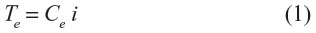
where C_e is a constant. According to the data sheet for the drill, the measurement range of the current sensor is 0–2.5 A.

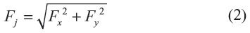
The force sensor was used to measure the normal cutting force at the milling surface. A sleeve was added in front of the drill handle. Through a sliding bearing installed in the front of the sleeve, the normal cutting force F of the drill bit can be transferred to the sleeve (Figure 2). Four strain gauges were bonded onto the sleeve; these could measure the radial force F_j, which is close to the normal cutting force F, by measuring the elastic deformation that occurred on the sleeve. The force sensor could measure two orthogonal component forces of the radial force F_j, F_x and F_y, wherein F_x represents the relatively horizontal component force and F_y represents the relatively vertical component force. The radial force F_j is calculated as follows:

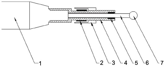Figure 2 Force sensors on the sleeve. Notes: 1, hand shank; 2, strain gauge; 3, protective shield; 4, sleeve; 5, sliding bearing; 6, drill pipe; 7, drill bit.

The measurement range of the force sensor is from −5 N to 5 N, with a resolution of 0.005 N and an accuracy of 0.05 N.

As the rotating drill bit may stir up blood or other corrosive liquids, the strain gauges and signal conditioning circuit are covered in protective casing (Figure 3). The sample rate of each sensor signal channel is 1,024 Hz. To suppress sensor noise, an oversampling method is used.¹¹

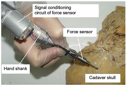Figure 3 Modified drill system.

The grinding object used in the experiment was calvarial bone that had been fixed in formalin. Ethical permission for use of the bone sample was given by Peking Union Medical College Hospital. All the experimental data were accessed and processed by a computer.

Data preprocessing

The original signal from the sensors contains a lot of noise and interference. And we use DB2 wavelet transform and reconstruction as a denoising method.

Since the original data, as well as the wavelet processed sample data, were oversampled, a mean filter is used:

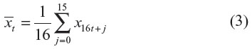
where represents the input data of the recognition method at time t, updated every 0.0156 seconds, and x_16t+j denotes the sample data processed by DB2 wavelet. After the average-filtering, the frequency of the input data was decreased from 1,024 Hz to 64 Hz. However, the data preprocessing has not ended.

One thing we know is that the values of the force sensors do not correspond to zero when the drill is idling, since readings from the force sensors can be influenced by the weight of the drill bit. During surgery the drilling angle is changing all the time, so the readings of the force sensors during idling periods are not constant.

However, if we want to calculate the normal cutting force F more accurately, we need to remove the influence of the weight of the drill bit. Therefore, the readings of each force sensor, F_x or F_y, should be preprocessed. We can calculate the average values of each force sensor before a drilling maneuver, and set it as a base value for the following force signals. The reversed force signal is the difference between the original signal and the base value. The readings of force sensors before every drilling operation change but the readings of the current sensor do not, so we can judge whether the drill is idling by the readings of the current sensor. The collation map of the initial and reversed force signal of F_x or F_y are shown in Figure 4.

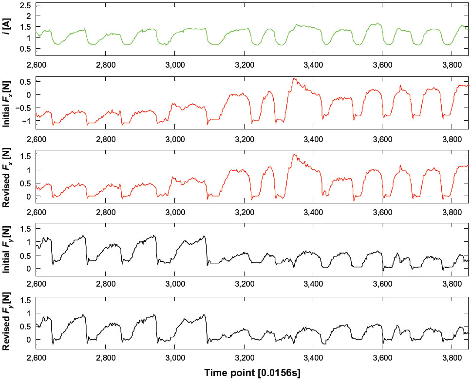Figure 4 Collation map of the initial and reversed force signal of Fx and Fy. Note: The data in this figure were collected in the process of normal milling.

Mathematical model of the DC motor

The essential to find the relationships between the force signal and the current signal lies in the mathematical model of the DC motor. According to the properties of the DC motor, the change rules of the armature current and the motor speed can be described by the following equations:¹²

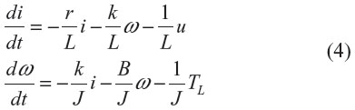
where i is the armature current, u is the armature voltage, r and L are the equivalent resistance and equivalent inductance of the armature winding, k is the torque constant determined by the permanent magnet and armature magnetic properties of the motor, B is the coefficient of frictional resistance of the motor rotor, T_L is the torque of the rotating load, ω is the rotor angular velocity, and J is the total moment of inertia of the motor rotor and the drill bit.

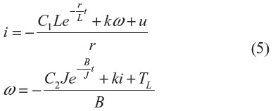
The solutions of the differential Equations 4 are shown in Equations 5, where C₁ and C₂ are constants.

After eliminating the ω, we obtain the expression of i :

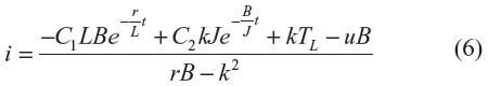
To obtain the relationship between the armature current i and the torque of the rotating load T_L, we write Equation 6 as below:

where C₁ to C₆ are constants, and differ from those in Equation 6. The first two terms on the right side of the equation are exponential terms, which decrease with time. Their existence can be revealed by the armature current (Figure 5). The current signal right after turning on is a little higher than that during idling.

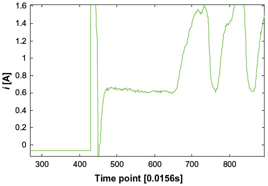Figure 5 Current signal after starting the drill, when we find a slow decline in the current. Note: The data in this figure were collected in the process of normal milling.

If we use i to express T_L, and ignore the exponential terms, Equation 7 can be written as follows:

where C_{k 1} and C_k2 are constants.

Since the drill bit is slipping on the bone surface during milling, the milling force can be recognized as sliding friction. Its value f depends on the surface materials and the normal pressure F_N. The expression of f is shown below:

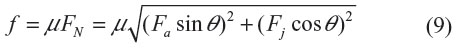
where μ is the coefficient of sliding friction, θ is the angle between the axis and the grinding surface, F_a is the axial force, and F_j is the radial force.

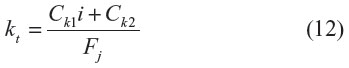
During a normal milling operation, the axial force is usually much smaller than the radial force, so we assume that T_L during normal milling is in proportion to the radial force F_j, and this relationship can be described as follows:^13,14

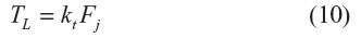
where k_t is a coefficient that depends on the physical properties of the grinding object. The higher k_t is, the harder the object could be. The value of k_t can be changing, while the value of F_j can be measured by the current and value of k_t. From Equations 8 and 10, we derive the following equation:

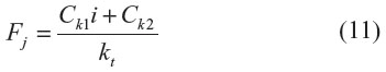
Since every term in the right side of Equation 11 has its coefficient, we set the value of k_t to be 1 during normal milling, so that it will be easier to compare values between normal milling and abnormal milling.

Next we use Matlab to fit these two coefficients, C_k1 and C_k2, through the current and force data during normal milling. The scatter diagram of the fitting outcome is shown in Figure 6.

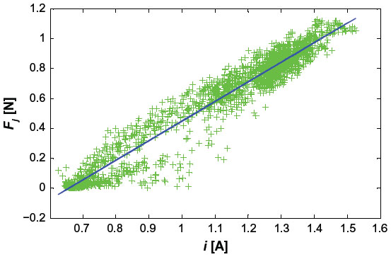Figure 6 Scatter diagram of Fj and i during normal drilling and their fitting curve.

Phase difference and its influence

Now we can use the coefficients fitted by the data collected from normal milling, C_k1 and C_k2, to calculate the curve of k_t. The value of k_t is expected to be around 1, and its expression is shown in the following formula:

To avoid sharp fluctuations of k_t when the value of F_j is near zero, we add a small constant to the denominator of the expression above, and to keep the average value of k_t, the same constant is also added to its numerator. Now the expression of k_t is:

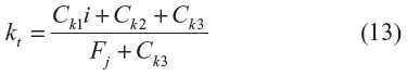
Here the constant C_k3 =0.05

The curve of k_t during normal milling is shown in Figure 7. We can see easily that when F_j increases rapidly, k_t will suddenly decrease, and when F_j decreases rapidly, k_t will suddenly increase. As the increasing speed of F_j at the beginning of each milling is higher than its decreasing speed at the end, the amplification of k_t at the beginning is larger than its damp at the end of each milling.

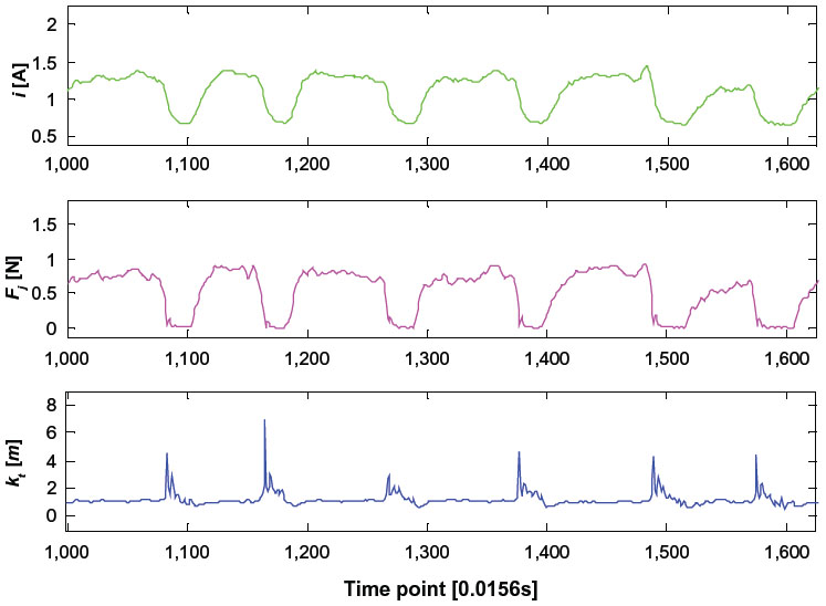Figure 7 Comparison of i, Fj and kt during normal milling. Notes: The data in this figure were collected in the process of normal milling. The dimension of kt is determined according to equation (10).

Cao at the University of Science and Technology Beijing identified a phase difference between the force signal and the current signal. During normal milling, the force signal changes a little earlier than the current signal. However, when the bone wall is being milled through, or the drill is entangled with a cotton swab, the current signal seems to change earlier than the force signal.¹⁵

This phenomenon can be explained by Equation 5 and the curve of k_t during normal milling (Figure 7). There is an exponential term about time in the rotate speed expression of Equation 5, and the variation amplitude with time of this exponential term depends on J and B, the moment of inertia, and the coefficient of frictional resistance of the motor rotor.

From Figure 7 we find that when the status of the drill changes from idling to milling, the value of k_t will suddenly decrease. This is because when the resistance to the drill bit increases rapidly, and the rotation speed decreases rapidly, some of the rotational kinetic energy of the drill will help the electrical energy to overcome the resistance, so the current increases relatively slowly. As a result, the value of k_t declines rapidly.

Likewise, the value of k_t will suddenly increase while the status of the drill changes from milling to idling. This is because when the resistance decreases rapidly, the current signal decreases more slowly than the force signal.

However, we should take note of the fact that the discussion above is reasonable only in the following precondition, ie, when all the load resistance comes from frictional resistance, ie, the status of the drill must be normal milling, because only in this circumstance can the resistance to the drill bit be in proportion to the value of force sensor signal.

When the drill bit is entangled with a cotton swab or is milling through the bone wall, there will be further resistance besides milling force. At this time, the delay in the current signal when compared with the force signal seems to decrease, and even reverse. This phenomenon is consistent with the research reported by Cao.¹⁵

However, Cao did not offer an explanation for this phenomenon, and used a moving average filter to eliminate the influence of the phase difference, regarding it as a measurement error. In fact, the phase difference should be constant as long as the DC motor has not been changed. We can treat this as a systematic error, so that we can take more advantage of the information from sensors.

Eliminating the influence of the phase difference

From the discussion above, we know that k_t is a key parameter in distinguishing whether the state is abnormal, and k_t can be influenced by the phase difference between the current signal and the force signal. To eliminate the influence of phase difference, we attempted the following steps.

First, differentiations are done to both sides of Equation 7, and we obtain:

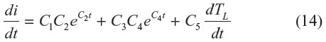
According to Equation 14, the rate of change in current i and that of T_L only differs by two exponential terms, and Equation 6 shows that both these exponential terms decrease with time, ie, if we shift the time axis of current i to an earlier time, the rate of change in current i will be approximately in proportion to that of T_L.

Now the question becomes how long time we shift earlier the time axis of current will make the change rates of i and T_L close to a proportional relationship? We think that this happens when the variance of the k_t array reaches the minimum value, ie, when the following function f(m) with the independent variable m also has the minimum value:

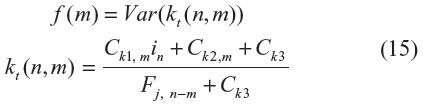
Here k_t(n,m) is a two-dimensional matrix, where n is the point in the time array; its value is a positive integer, and m is the number of time points by which we shift earlier the time axis of current i, or we shift later the time axis of F_j. i_n is the value of the current sensor at time point n, and F_j,n-m is the composition of F_x and F_y in time point n-m. C_k1,m and C_k2,m are the coefficients fitted by the shifted data, i_n, i_n+2, i_n+2… and F_j,n-m, F_{j, n-m+1}, F_{j, n-m+2}… which are collected from normal milling. As the frequency of the data is 64 Hz, the time between the two nearest time points is 1/64 of a second.

When m values from 0 to 80, integer only, the functional relationship between f(m) and m is shown in Figure 8. It is obvious that when m =2, approximately 0.03 seconds that we shifted earlier the time axis of current i, f(m) will have a minimum value.

Figure 8 Functional relationship between f(m) and m, where the horizontal ordinate represents m and the vertical ordinate represents f(m).

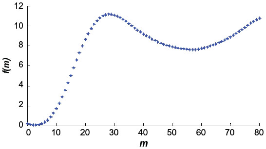
We compared the curve of k_t when m values were 0 and 2, and the result is shown in Figure 9. We can see easily that when the m value is 2, the influence of the lag of the current signal brought to k_t has almost been eliminated. And now the value of the coefficient C_k1 is 1.3263 and that of C_k2 is −0.8789.

Figure 9 Comparison of the curve of kt when the m values are 0 and 2, where the horizontal ordinates represent time points and the vertical ordinates represent kt.

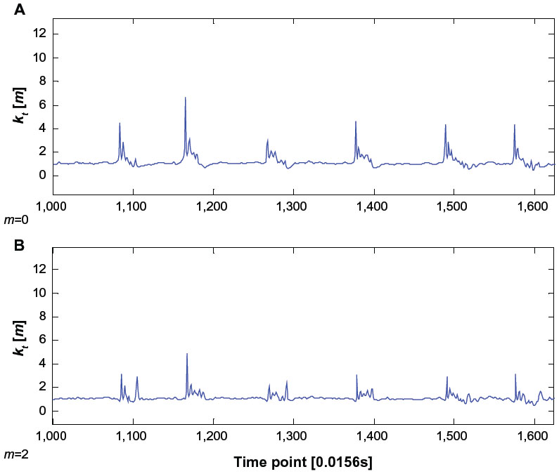
Although when m values 2, f(m) has a minimum value if m must be an integer, what if m equals a decimal number? To obtain a more accurate m, we can linearly interpolate the force data that will be used to fit coefficients. From the results above, we know the value of m we want is between 2 and 3. So the force data that are shifted earlier by time point number m can be calculated by the following expression:

We set the interval of interpolation to 0.02, and then calculate the 51 values of f(m), the result of which is shown in Figure 10. When the m value is 2.42, f(m) reaches a minimum value.

Figure 10 Curve graph between f(m) and m for m values of 2 to 3, where the horizontal ordinate represents m and the vertical ordinate represents f(m). Note: f(m) is a function defined by equation (15), and m is the number of time points by which we shift earlier the time axis of current i, as is mentioned in this article.

Through Figure 11, we can find that the fluctuation of k_t when the m value is 2.42 is smaller than that when the m value is 2. Now the coefficient C_k1 value is 1.3240 and the C_k2 value is –0.8763. Since the coefficients are both determined by the properties of the DC motor, but not the grinding object, use them as a couple of standard coefficients in the next.

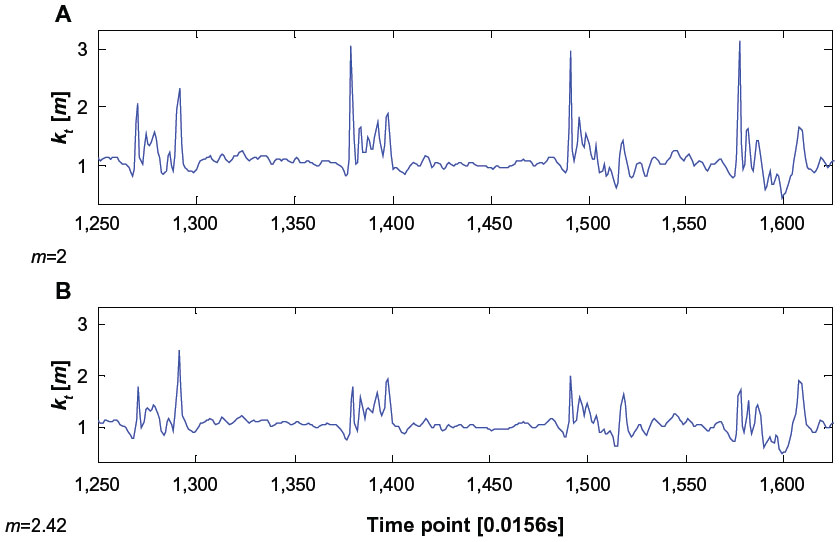Figure 11 Comparison of the curve of kt for m values of 2 and 2.42.

Since the value of k_t is unstable when the current decreases rapidly, we need to eliminate this interference. Here we do a revision to the calculation of k_t to make it more smooth and steady when the current decreases rapidly. At the same time, we add a larger number to the denominator of the expression of k_t to make it steadier during idling. So k_c, the correction value of k_t, can be calculated by the following equation:

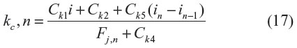
where C_k4=0.2, C_k5=1, and k_c,n, i_n, and F_j,n are the values of k_c, I, and F_j in moment n.

Recognition algorithms

According to the surgeons’ operating habits and the experimental data, the rate of change in the current during normal milling is usually small, not exceeding 5 A per second. However, when milling through the bone wall, the rate of change can reach 2 A per second. The reason for this is shown in Figure 12. When the bone wall is being milled through, the rotating concave bit will meet the edge of the bone cavity, which can prevent the bit from rotating rapidly, and has a larger resisting moment to the bit. The duration is short but the feature is remarkable.

Figure 12 Sketch of the drill bit when it is milling through the bone wall.

We should set thresholds for the current rate of change to judge whether the bone wall is being milled through. Here the thresholds, including the upper threshold and the lower threshold, are determined by , the average increment rate of the current signal during normal milling. When the increment rate of the current signal is positive, we can use it to calculate the average value.

Likewise, the thresholds for the increment rate of k_c, including the upper threshold and the lower threshold, are determined by , ie, the average increment rate of k_c during normal milling. Further, when the increment rate of k_c is positive, we can use it to calculate the average value.

Both and should be continuously revised during the milling operation.

The final recognizing algorithm for milling through the bone wall can be realized by a piecewise function. We use the function P_th,n to represent the chance of milling through by time point n.

The value of P_th,n is the summation of two parts, one determined by the increment rate of i and the other by the increment rate of k_c; both parts have equal weighting. For either of the two increment rates, if it is smaller than its lower threshold, then it will contribute zero to the value of P_th,n; if it is between the lower and upper thresholds, its contribution to P_th,n will change from 0 to 0.5 linearly; if it is larger than the upper threshold, it will increase the value of P_th,n by 0.5. That is to say, if the increment rates of both i and k_c reach their upper thresholds, the value of P_th,n will be 1.

The expression of P_th,n can be described by Equation 18.

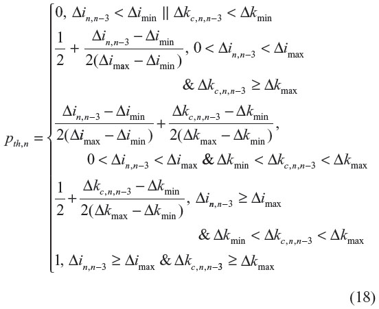
where Δi_min, Δi_max, Δk_min, and Δk_max are all thresholds determined by and . Δi_n,n–3 = i_n – i_n–3, Δk_c,n,n–3 = k_c,n – k_c,n–3, where i_n and k_c,n represent the value of i and k_c at time point n. If P_th,n is >0.5, milling through bone wall will be predicted to happen by the system.

When the drill bit is entangled by a cotton swab, it is not a remarkable feature that the current signal increases rapidly, but k_c increases quickly. Of course, the current signal will certainly increase in this period because of the extra resisting moment brought about by the cotton swab.

The final recognizing algorithm for entanglement with the cotton swab can also be described by a piecewise function. We use P_wr,n to represent the chance of entanglement in time point n.

This time, we set a smaller lower threshold for the increment rate of i, and a lower and upper threshold for that of k_c.

If the increment rate of i is smaller than its lower threshold, then P_wr,n will get the value of zero, and the system will not predict that the entanglement is happening; as long as the increment rate of i is larger than its lower threshold, P_wr,n will depend on the increment rate of k_c, and values of 0 to 1 linearly with the increment rate of k_c values from its lower threshold to its upper threshold. If the increment rate of i is larger than its lower threshold and the increment rate of k_c reaches its upper threshold, the value of P_wr,n will be 1.

The expression of P_wr,n can be described by Equation 19.

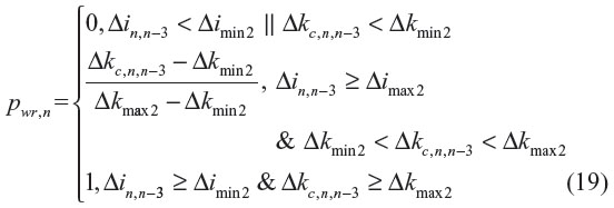
where Δi_{min 2}, Δi_{max 2}, Δk_{min 2} and Δk_{max 2} are all thresholds determined by and . Δi_n,n–3 = i_n – i_n–3 and Δk_c,n,n–3 = k_c,n – k_c,n–3, where i_n and k_c,n represent the value of i and k_c in time point n. If P_wr,n is >0.5, entanglement with cotton swab will be predicted to happen by the system.

Results

We have done tests to prove the effectiveness of the recognition algorithms presented above using the experimental data collected from five surgeons.

During 500 experiments of milling through bone tissue wall by five doctors, 465 of them in total were recognized successfully. The recognition rate was 93%. When we used the judgment function for milling through bone wall in 250 times’ normal millings, only five times in total were recognized as milling through bone tissue wall. The error rate was 2%.

As a result, we can say that the recognition algorithm for milling through the bone wall is effective. The recognition of milling through the bone tissue wall is shown in Figure 13.

Figure 13 Recognition of milling through bone tissue wall. Note: The data in this figure were collected in the process of milling through.

During 250 times’ experiments of milling entangled by cotton swabs by five doctors, a total of 230 of them were recognized. The recognition rate was 92%. And when we used the judgment function for entanglement in 250 times’ normal millings, only 2% of them were unexpectedly recognized as entanglement. The error rate was 2%.

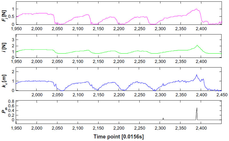
As the result, we can say that the recognition algorithm for entanglement with cotton swabs is effective. The recognition of entanglement is clearly shown in Figure 14.

Figure 14 Recognition of entanglement with cotton swabs (the data in this figure was collected in the process of entanglement).

The final results of the recognition method for milling through the bone wall and entanglement with cotton swabs are shown in Table 1.

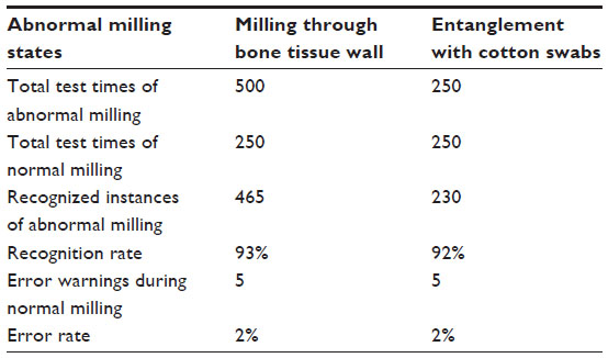Table 1 Final results of the recognition method for abnormal milling states

Discussion

This paper presents a new method for identifying the milling state of an otological drill. This multi-sensor based otological drill system could be adapted for individual surgeons and identify the early stage of milling through a bone tissue wall or entanglement with a cotton swab in a timely and accurate manner, with few false alarms during the normal milling process. This identification method could assist surgeons when performing otological procedures with fewer unexpected injuries to patients.

Our final discriminant for milling through contains two indices, ie, the rate of change of k_c and that of the current signal. During normal milling, if the current signal increases rapidly only because the surgeon presses hard suddenly, the value of k_c will not undergo a sudden change. However, when the drill bit is milling through the bone wall, there will be not only a sudden increment of current signal, but also an obvious increment of k_c because of the increased resistance. Surgeons usually operate carefully, so it seldom happens that the current signal increases suddenly during normal milling. However, to ensure accuracy, k_c is calculated and plays a complementary role.

Since the signals in the period of milling through and entangling have something in common, so we use the change rate of k_c as a recognition judgment for both of them. As a result, some of the signals may fit both of the recognition algorithms. This will not hinder the decision whether to stop running, since the system just needs to distinguish whether the milling state is normal or abnormal. When milling is normal, the drill keeps running until the surgeon turns it off, and when milling is abnormal, the drill will turn itself off automatically.

If you want to differentiate between milling through and entangling, you can delay the time of judging, so that their differences will come out. However, when using this intelligent system, it is essential to recognize the abnormal state as soon as possible, so we prefer to identify whether the state is abnormal immediately then tell which kind of abnormal state it is.

The final recognition rates for the abnormal milling states, which were expected to be 100%, are just larger than 90%, so the recognition methods need further improvement.

The reason for the errors in recognition of milling through perhaps lies in the thresholds, because sometimes the demarcation line of the selected indices between milling through and normal milling are not clear. For example, if the extra resisting moment acted on the concave bit by the bone cavity is not large enough during milling through, the recognition function may give a wrong result. Similar reason can be used to explain the recognition errors of entanglement.

The indices in our final discriminants did not include change in force direction, which may also aid recognition of milling states. The only use of the two-dimensional force sensor was to calculate the resultant force, but the force direction was ignored, which may be useful to reduce the error rate.

Acknowledgment

This work was funded by the National Key Technology R&D Program (2012BAI12B01) for China’s 12th Five-year Plan Period.

Disclosure

The authors report no conflicts of interest in this work.

---

References

1.	Green JD, Shelyon C, Brachmann DE. Iatrogenic facial nerve injury during otologic surgery. Laryngoscope. 1994;104:922–926.
2.	Shen P, Feng G, Cao T, Gao Z, Li X. Automatic identification of otologic drilling faults: a preliminary report. Int J Med Robot. 2009;5:284–290.
3.	Cao T, Li X, Gao Z, Feng G, Shen P. A method for identifying otological drill milling through bone tissue wall. Int J Med Robot. 2011;7:148–155.
4.	Cao T, Li X, Gao Z, Feng G, Shen P. An intelligent monitor system of otologic drill to prevent drill bit entangling with the cotton. Proceedings of the 2010 IEEE International Conference on Information and Automation, June 20–23, 2010, Harbin, People’s Republic of China.
5.	Ong FR, Bouazza-Marouf K. Drilling of bone: a robust automatic method for the detection of drill bit break-through. Proceedings of the Institution of Mechanical Engineers, Part H. Journal of Engineering in Medicine. 1998; 212:209–221.
6.	Ong FR, Bouazza-Marouf K. The detection of drill bit break-through for the enhancement of safety in mechatronic assisted orthopaedic drilling. Mechatronics. 1999;9:565–588.
7.	Lee W-Y, Shih C-L. Control and breakthrough detection of a three-axis robotic bone drilling system. Mechatronics. 2006;16:73–84.
8.	Hong J, Matsumoto N, Ouchida R, Komune S, Hashizume M. Medical navigation system for otologic surgery based on hybrid registration and virtual intraoperative computed tomography. IEEE Trans Biomed Eng. 2009;56:426–432.
9.	Dillon NP, Balachandran R, Motte dit Falisse A, et al. Preliminary testing of a compact bone-attached robot for otologic surgery. Proc Soc Photo Opt Instrum Eng. 2014;2014:903614.
10.	Li X, Xie Y, Gao Z, Feng G. A smart recognition method for otological drill milling through a bone tissue wall. Available from: http://www.scientific.net/AMM.571-572.331. Accessed March 25, 2015.
11.	Sandler EA, Gusev DA, Milman GY, Podolsky ML. Estimating from outputs of oversampled delta-sigma modulation. Signal Processing. 1997;59:305–311.
12.	Nasar SA, Unnewehr LE. Schaum’s Outline of Theory and Problems of Electric Machines and Electromechanics. 2nd ed. New York, NY, USA: McGraw-Hill; 1997.
13.	Zaman MT, Senthil Kumar A, Rahman M, Sreeram S. A three-dimensional analytical cutting force model for micro end milling operation. International Journal of Machine Tools and Manufacture. 2006;46:353–366.
14.	Kang IS, Kimb JS, Kim JH, Kang MC, Seo YW. A mechanistic model of cutting force in the micro end milling process. Journal of Materials Processing Technology. 2007;187–188;250–255.
15.	Cao T. Study on multi-sensor information fusion monitor system of otological drill (Dissertation). Beijing, People’s Republic of China: University of Science and Technology Beijing; 2012.