Modeling Trade Openness and Life Expectancy in China

Introduction

Trade Openness has multidimensional implications on the economy, environment, and human health. Trade openness expands industrial production, which increases the income and welfare of the people in the economy.¹ The rise of income due to the trade expansion improves the standard of living and people may adopt a healthy lifestyle and better maintain health quality thus leads to improve life expectancy.^2–4 Besides the positive effect of trade, there is also a negative effect of trade openness mainly due to CO₂ emissions in society. Trade activities increase CO₂ emission in three different ways; scale effect, composition effect, and technique effect.^5,6 The scale effect represents the increase in CO₂ emissions as a result of trade liberalization and the rise of industrial production, especially in the export sector industries.^7,8 The composition effect arises due to change in the production pattern and comparative advantage which implies that industries specialize in those products in which the country has a comparative advantage. The technique effect is the final channel through which trade increases CO₂ emissions and it indicates that post-trade openness countries change production patterns towards more technological modes, consequently leading to higher CO₂ emissions in the economy.⁷ The trade liberalization could potentially increase CO₂ emissions unless its embodied regulations control greenhouse-gas in production.

Carbon dioxide emissions reduce environmental quality and negatively affect human health and labor productivity.⁹ CO₂ emissions are the major cause of influencing environmental quality that adversely affects life expectancy. The medical research found different types of mortalities resulted from environmental pollution, for example, small particulate matter causes work loss and bed disability in adults.¹⁰ Different pollutants like sulfur dioxide and total suspended particulate (TSP) increases mortality rates.¹¹ Trade openness increases the CO₂ emissions leading to reduces air quality which resulted in a low level of life expectancy.^7,12,13 There is a causal link between life expectancy and environmental quality; several studies in medicine and epidemiology, like Elo and Preston;¹⁴ Pope¹⁵; Evans and Smith¹⁶ show that poor environmental quality leads to reduces life expectancy.

Trade openness is an important driver of progress, skill transfer and productivity among the regions of the world. Hence, enriched literature is available on various aspects of the impact of trade openness on economic growth, income distribution, government spending and environment. However, there is little known about the effect of trade openness on physical heath. To the best of our knowledge none of the published studies so far have examined the relationship among trade openness and life expectancy by using long time series data for the period 1960–2018. Therefore, this study will fill the narrow gap by investigating trade openness on life expectancy using China as case study for the period 1960–2018.

China has a significant contribution both in world trade and CO₂ emissions; trade activities could potentially influence the CO₂ emissions in China therefore this study aims to explore the relationship between trade and life expectancy in China for the period 1960–2018. Furthermore, there is no clear theoretical model that links trade openness with life expectancy, hence we firstly construct a theoretical model that linking trade implication of trade openness for life expectancy. Secondly, we will test our theoretical model by using the regime-switching regression method and further verify our baseline results by applying the Granger causality test and OLS for the robustness of our results. Our theoretical model covers both aspects of trade implication for life expectancy and it could provide detailed policy insight to policymakers and stakeholders to improve trade policy and reduces the negative implication of trade openness in China.

The rest of the paper structure is as follow: Trade, CO2 and Life Expectancy in China presents the theoretical framework of the study: In Methodology and Model we briefly describe Trade, CO₂ and Life Expectancy in China: Results and Discussion presents the methodological approach used in the study. Conclusion conclude the study.

Theoretical Framework

Following the Bernard et al¹⁷ model for CO₂ emissions and trade, the initial equation shows consumer preferences for a good produced in-country d and consumed in-country j. the consumer presences can be presented as follow.

Consumption

(1)

(2)

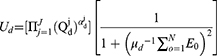
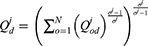
The model further assumed a world of N countries, a representative agent, and a fixed labor supply. Equation 27 shows the utility function for the consumption of the traded commodity transported from country O to country D. The second equation indicates the disutility due to the CO₂ emissions due to the trade activities.¹⁸ The term shows CES aggregate of varieties which indicates trade from origin country o to destination country d of sector j goods. The is elasticity of substitution between sector j varieties, which is greater than 1.⁷ The constant elasticity substitution preferences across the sectors show that the country d spends a share on j sectors. The Eo is social cost represented by CO₂ emissions from country o. It is assumed that production requires labor as a single factor, CO₂ emissions are assumed as a pure negative externality, which decreases the utility but it does not affect the trade. Equation 27 show that the increase in the total quantity of products transported from country O to country D will increase the utility while the increase of the quantity of CO₂ emission will decrease the utility. The price index under for sector j in country d under these assumptions could be represented as follow

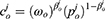
This equation is similar to the utility equation and its total price of sector j from country O to country D. Where is the total price of sector j, shows the price of sector j from o country to d country. The local price is assumed 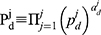, this price index does not contain CO₂ (social cost) and it follows the assumption that CO₂ emission is pure externality.^19,20 The indirect utility function is presented as follow

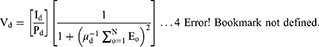
This indirect utility equation shows that social welfare²¹ is determined by real income ( and environmental damage (to the country.²² Besides, each country has a different willingness-to-pay for restriction of CO₂ emissions, this implies that income is devoted to get in a country.

Production

The production function follows iceberg form as follow

(3)

(4)

By using Cobb–Douglas Function with the share of labor and intermediate goods, the production cost can be subdivided into wage and the prices of intermediate goods. The product price at destination country d can be divided into the product price and the trade cost. Since the trade cost relates to the product cost follows as a continuous variable, so we use the direct product rather than the Cobb–Douglas Function. Where are wages of the labor, is the price of intermediate, is the production cost : the labor price ( is the share of labor) : the price of intermediate goods, is the share of intermediate goods : the product price at destination country d : trade cost. Besides, we can add the share of each factor (containing the environment) by following the Cobb–Douglas.

(5)

Total Trade Cost

(6)

(7)

The equations represent that trade cost can be influenced by factors like carbon tax, fuel cost and all types of trade frictions.²³ The trade costs contain the distance between countries , the share of trade in dollars , the weight-to-value ratio for goods , the fuel efficiency, the carbon tax rate for imports and exports, where γ is the constant term. 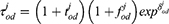The total fuel cost can be composed by the distance between countries , the share of trade in dollars , the weight-to-value ratio for goods , the fuel efficiency , the global oil price , while γ is the constant term. The total cost can be represented by the form (1+t) and all bilateral trade frictions are combined by using the exponential form given in equation 7.

Environment

The transitional effect of trade on the environment is illustrated as following

(8)

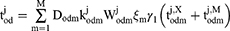
The Ed is social cost represented by CO₂ emissions from country d. It can be divided into fuel, CO₂ emissions from the transportation sector, and CO₂ emissions from the production sector (). Where shows the fuel cost per dollar of expenditure, is tons of CO2 emitted per dollar of fuel. presents the units of goods produced in the country o and consumed in-country d. : the CO₂ emissions per unit of output for sector j in country o.

Health

Human health is the main factor that affects life expectancy and quality of health ensures the longevity of human life. The health quality of life is determined by various factors including healthcare facilities, income, CO₂ emissions. The availability of proper healthcare facilities, the income level of the individual could have a positive influence on health quality, while CO₂ emissions have a negative relationship between health quality.

(9)

(10)

(11)

(12)

Besides the healthcare facility, the equity issue is also one of the main concerns to government stakeholders. To allow the health-income inequality in the model, we follow Van Doorslaer et al²⁴ concentration index and Lorenz curve. Equation 11 shows the curve in the health quality; it is based on two upper and lower ranges such as 1, −1, with 0 which represents the perfect equality in health quality. The second equation shows a concentration index based on the health score and health rank , there is a however negative relationship between health score and health rank. Besides, the effect of health scores is assumed to influence at a slower rate. Equation 3 captures the health score is determined by health factors with coefficients. The equation 4 concentration index represents the health factors and generalized concentration index .²⁵

Health Quality and Healthcare Facility

(13)

Preposition 1

A part of the income is devoted to healthcare facilitates.

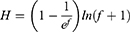
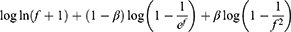
This equation demonstrates the relationship between health quality and healthcare facilities, where f shows the quantity of the social facility and H: The health quality.²⁵ Since trade liberalization increases the overall economic income and it is assumed that a part of income is allocated to the healthcare facility. The equation shows that’s trade activities initially improve the health quality due to an increase in the income and later it decreases the health quality due to the high environmental cost in terms of pollution particularly the CO₂ emissions from the production and export sector. However, in the long run, the health quality will remain constant.

Health Quality and Income

(14)

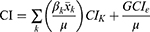
According to the CI in equation 12

Health quality significantly determined by income; people may spend a sufficient amount on health thus maintain health quality. However, equity in the healthcare sector is the main factor influencing health quality along with income factors. The model uses Van Doorslaer et al²⁴ concentration index to evaluate the health quality and income holding the inequality factor. The health concretion index contains a healthy score of people (), the healthy rank of individual R_i and income, average of health and income . The equation 16 depicts that health quality positive effect on the health quality keeping constant the inequality healthcare services.

Health Quality and CO₂

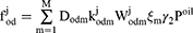
CO₂ emission linked with four aspects: population, per capita income, energy intensity, and carbon intensity effect.¹³ The trade activities increase the CO₂ emission in the economy that consequently leads to an adverse implication on the health quality of society.²⁶ The Ed is a social cost containing CO₂ emissions from country d. using equation 10 the social cost E_d and CO₂ emissions relationship as follow

(15)

This equation represents the CO₂ emissions have an adverse effect on human health and this exponential form is used as CO₂ emissions have a stronger effect on human health. The relationship between CO₂ emissions and humans has been testing by various studies including Mohmmed et al;¹³ Chaabouni and Saidi;²⁷ Chaabouni et al;²⁸ de Koeijer et al²⁹ they found the CO₂ emissions harm human health.

Life Expectancy

Life expectancy is determined by several factors including “healthy lifestyle, education, body mass index (BMI) and healthcare facilities, and routine diet„.³⁰

Life Expectancy and Healthy Lifestyle

(16)

The equation represents a healthy lifestyle and life expectancy. The factor that determines the healthy lifestyle includes the smoking (X1), drinking (X2), physical activities (X3) (excise), good sleep (X4) and proper food (X5).³¹ The equation follows the normal distribution and we assumed a mean value 1 unit for all the factors. Physical activities, good sleep and daily food are positively affecting factors denoted by respectably. While smoking and drinking negatively influencing factor denoted by . X is taken as average of these factors; the standard normal distribution is used to describe the average of X and any deviation in these factors is easy to observe by comparing with the mean value of X.

Life Expectancy and Education

(17)

Life expectancy depends on the education (X) of the individual as education could provide awareness and importance of quality of health.³² Although education is an important factor however it may not be the primary factor influencing life expectancy therefore, we use log function, while t is constant shows any change in the function. This equation depicts that education could improve life expectancy by adopting a healthy lifestyle.

Life Expectancy and BMI

(18)

The body mass index (BMI) is used to measure the height and weight of the individuals. t shows the total number of the people, it calculated by taking the ratio of weight in Kilogram) to the height (in meters) of individuals. For adults, an ideal BMI is in the 18.5 to 24.9 range. This depicts that if the induvial BMI ratio exists at the rate of 18.5 to 24.9 then it following the health status and improved life expectancy. Since it is symmetric in the interval between [18.5, 24.9] therefore for equation 20 we use the normal distribution to measure the BMI, and confidence interval provides information of variations in BMI.

Life Expectancy and Facilities

(19)

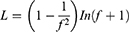
Where f shows the healthcare facilities including availability of doctors, hospitals and medical units, etc. and L shows the life expectancy. The health care facility is the primary determent of life expectancy. The increase in healthcare facilities increases the life expectancy of the individual.³³ This equation depicts the with no healthcare facility a low level of life expectancy is observed. Health quality increases with the increase of social facilities. It is assumed that a healthcare facility holds a diminishing marginal rate property, which implies that it increases the life expectancy to a certain level and it does not improve the life expectancy beyond a specific level.

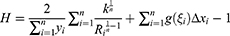
Life Expectancy and Income

(20)

Where shows the mean healthy score, health rate index of individual K parameters, Income index, and D are the domain of income function. Income is the most influencing factor that affects health as well as health quality. The equation presents a significantly larger impact on health quality compare with life expectancy. The equation depicts individual life expectancy as an additive function to human health with then rises positively affecting life expectancy.²⁵

Life Expectancy and Diet

(21)

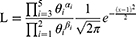
The diet is one important factor affecting life expectancy, the calories level (C) and nutrition (N) has a positive effect on life expectancy while smoking () has a negative effect on life expectancy.³⁴ The function follows the Cobb–Douglas function and β_j is the share of calories. Besides, the exponential form of denominator factors indicates that smoking could have a wider effect as compare to nominator factors.

Now Combining the health and environment factors in life expectancy equation as

L = f (Environment factors, Health factors)

(22)

The equation 24 presents the life expectancy is determined by environmental and health factors. CO₂ emissions are the main responsible factor for degrading health quality which resulted in lower life expectancy. However, trade activities raise the income of the people which allocated to maintain health leading to improves the health quality and thereby increase the life expectancy. However, the net effect of trade on life expectancy primarily depends on the rise in income and environmental cost (CO₂ emissions). The trade and life expectancy equation could be further extended to the developing and developed country cases.

Developed Countries

(23)

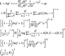
The developed countries may have diverse effects as compared to the developing countries due to differences in economic, political, and institutional structure. Since developed economies gain from the trade by better utilization of their resources that sufficiently compete for the country’s imports. For developed countries, we consider education, healthy lifestyle, income, social facilities, pharmaceutical, health quality and CO₂ emission, health expenditures, and institution quality factors that determine life expectancy. Know that health quality contains healthcare facilities, income, and CO₂ Emissions, we added some additional factors that differentiating the developed countries from developing countries. Since developed countries assumed to allocated sufficient funds for the health expenditures healthcare expenditures denoted by C1 and developing countries have the quality of institution denoted by C2 for the implementation of health policy. Lastly, we combine these factors in the life expectancy equation by following Cobb-Douglas function and the share of each factor represents by 1-α, α, 1-β, β, 1-γ, γ, 1-ᵟ and ᵟ. The logarithm form of the life expectancy equation could be expressed as

(24)

Since the Cobb–Douglas function is widely used in economies and convenient to differentiate the effect of each factor by using the partial derivative function. The partial derivative could be used to differentiate each influence on life expectancy. For example, the and provide any change in health expenditure (c1) and change in institution quality (c2). The “facility related to life expectancy” and facility-related to health quality can be represented by logarithm form as

(25)

Preposition 2: Developing countries allocate sufficient funds to the health sector (C1) and have a good quality of institutions.

Developing Countries

The developed countries may have diverse economic, political and institutional structures as compared to developing countries.³⁵ It is assumed that developing countries do not sufficiently contribute to the world market, nevertheless, the success of trade gains depends on the volume of exports against the volume of imports. In our model, we assumed developing and developed countries gains from the trade equally.

(26)

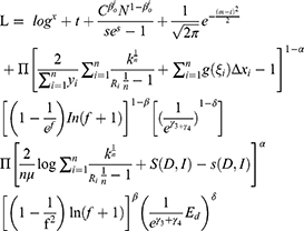
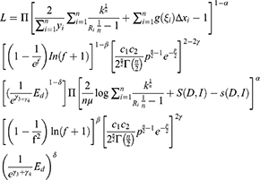
For developing countries, we omit C1 and C2 factors; as developing, economies spent a small amount on health expenditures (c1) and having poor institutions quality (2). We consider education, BMI index, diet, income, social facilities, health quality and CO₂ emission factors in the developing country case. The Cobb–Douglas function is used to combine these factors and share of each factor form as 1-α, α, 1-β, β, 1-ᵟ, and ᵟ. The data of the relevant variables are obtained from the World Bank online.

Trade, CO₂ and Life Expectancy in China

China has adopted Trade Openness in 2002 and made various trade reforms in history such as the open-door policy was initiated in 1978 to move the economy towards marketization and integration with the world market. In the early 1980s, China allowed a few foreign firms to operate in specific zones, and gradually reduces tariff from 1992 to 1996, most of the trade policies were import-competing. China’s export sectors were far ahead of its reform for its import-competing industries during the early 1990s and various export subsidies have suspended.³⁶ Besides other trade barriers, for example, import quotas and permits, authorization has been removed. China finally signs WTO in 2002 and a significant increase in the share of trade in the world. According to the Center for Strategic and World Bank (2015) the share of China in exports is13.45% in 2015 and attained double digits economic growth for the decade. Trade brings a substantial improvement in the income of the people and Figure 1 presents the trade openness and per capita income from 1960 to 2018. The per capita income was observed with a constant increase while trade shows a dynamic trend. The dynamic trend may result due to different factors including exchange rate, international recession. For example, during 2007–2008 there is a downward in trade which mainly resulted due to 2007 financial crises.

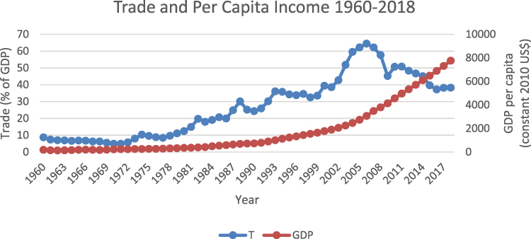Figure 1 Trade and per capita income 1960–2018. Note: World Bank Development.

Figures 2 and 3 represent the trade trend with CO₂ emissions and life expectancy, respectively. Trade activities are main especially industrial production as it accounts for 40.5% contribution in domestic production during 2017. This implies that industrial production major contributor to CO₂ emissions in China. Figure 2 shows the trend between trade and CO₂ emissions and there is a direct and increasing trend between Co2 emissions and trade. The overall increase in CO₂ emission with trade expansion indicates that trade activities main responsible factor for the CO₂ emissions in China. In 2008 a downward trend both in trade and CO₂ emissions occurred due to the international financial crisis the rest of the period shows a continuously increasing trend. Air pollution could have significant implications for human health and mortality. According to Ji et al³⁷ there were 7426 deaths reported due to air pollution between 2008 and 2014. Thus, on one hand, this graph depicts that trade contributed to human mortality by increasing pollution, while on the other hand, an increase in income from the trade could lead to attaining a high level of life expectancy. Figure 3 depicts trade and life expectancy trends, it shows the continuous constant increasing trend, while trade follows a dynamic trend. Trade has a dynamic effect on life expectancy which depends primarily on relative income effect and environmental effect, the net effect could provide a clearer scenario. According to Wu et al³⁸ PM2.5 potentially reduces the life expectancy in the urban population in China during 2013–2017.

Figure 2 Trade and CO2 emission 1960 to 2018.

Figure 3 Trade and life expectancy in China (1960–2018).

Methodology and Model

Model

We use the following model empirical analysis

Where ….

T is denoting trade

Lif is the life expectancy

GDP shows GDP per capita

CO₂ is the CO₂ emissions … GDP ….CO₂ …

Methodology

This section provides the method, which we are applying for the analysis, we adopted the regime-switching regression method for the analysis. Conventionally, liner regressions consider a primary tool for data analysis, however, there is considerable evidence of nonlinear modeling, especially when dealing with the macroeconomic analysis that is subject to regime change. Whereas nonlinearities arise from a discrete change in regime shift. In economic history, switching regimes models have been discussed by various researchers including Goldfeld and Quandt,³⁹ Maddala,⁴⁰ Hamilton and Susmel⁴¹ Frühwirth-Schnatter.⁴² Suppose that the time-varying variable follows a process that depends on the value of an unobserved discrete state variable and there are M possible regimes in the system, where state in line with regime m in t period when , where 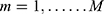. It is assumed that there are different regressions related to each regime. Suppose and are the regressors and conditional mean assumed to follow a linear specification;

(27)

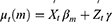
Where and are the coefficients for the and vectors, the coefficient is associated with regime change while is associated with and regime invariant. Furthermore, it is assumed that errors terms of the regressions are normally distributed

(28)

The error term is assumed normally distributed and the standard deviation of each error term depends on specific regime .

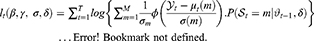
The likelihood can be formed by weighting the density function in each regime calculated by one step ahead probability in the specific regime.

, and determines the regimes probabilities, represents information set in period , while shows the standard normal density function. The full Maximum normal mixture can be presented in equation 3 that maximizes as follow

The regime probabilities are could be possible constant and varying values, for the constant values we could simply add additional parameters in the likelihood 4. For varying probabilities, we assume function of vectors of exogenous observables and the coefficient parameters by using multinomial logit specification.

(29)

The standard deviation , with the identifying normalization, . The special case of constant probabilities is handling by choosing ( to be identically equal to 1. In addition, we are taking two regimes, one pre-trade openness regime and the second is a post-trade openness regime and it exhibits implication of trade openness before and after trade openness in China for the life expectancy. Besides we will use some robustness checks such as standard Ganger causality and net effect model to further verify the bassline regime-switching estimations. The data for the relevant variables are obtained from the World Bank database for the period 1960–2018, which is freely available.

Results and Discussion

Baseline Estimations

This section provides the contains results and detailed discussion estimated by regime-switching regression. We constructed two regimes, first regimes contain estimations before the trade openness regime while second regimes show after the trade openness regimes. Table 1 presents descriptive statistics results; life expectancy and CO₂ emissions have a negative association, life expectancy with GDP reported a positive relationship with coefficient sign 0.64 and trade and life expectancy also found with a positive association.

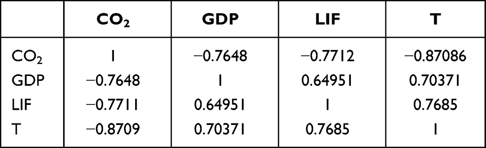Table 1 Descriptive Statistics

Table 2 presents the switching regime regression results; there are two regimes and each regime contains its coefficients with relevant significance. In the first regime, which is the pre-trade era the per capita GDP positively affects life expectancy at 1% level of significance. This indicates that with the rise in income level the life expectancy tends to increase and people adopt a healthy lifestyle and hold more income spend to maintain healthy life that resultantly leads to an increase the life expectancy. This confirms the Weixiang and Yu⁴³ findings as to the rise of income help people to attain health gains in China and thereby improving life expectancy. CO₂ emissions are reported insignificant influence on life expectancy, this indicates that CO₂ emissions have not main influence on the determination of life expectancy in the pre-trade liberalization in China. Moreover, this also indicates that fewer emissions are observed before the trade openness regime due to the lower level of industrial expansion in the country that does not influence life expectancy. Trade openness is insignificant at 5% level which implies that trade do not affect life expectancy in the pre-trade openness regime. It also indicates that there was a low level of trade activities including industrial production that leads to a low level of CO₂ emissions. Also, the low level of trade activities also does not contribute to the people’s income which confirms the insignificant association between trade and life expectancy. The second regime which is post-trade liberalization reveals interesting findings and implications of trade openness for life expectancy. In second regime GDP still hold significant implication for the life expectancy and GDP coefficient is significant at 5% level. This indicates that a rise in the income people leads to attaining good health which improves life expectancy, however unlike the first regime the GDP significant level move from 1% to 5%, which indicates the influence of other explanatory variables on life expectancy. CO₂ has a negative and significant effect on life expectancy at 1% level, which implies that CO₂ emissions have adverse implications for human health that lead to lower life expectancy. This study supports previous findings such as Ullah et al⁷, Ullah et al⁸, Hansen and Selte⁴⁴, Apergis et al⁴⁵, Ullah et al⁷ and Ullah et al.^8,46 Trade-in second regime positively affects life expectancy at 1% level of significance, which implies that trade activities could improve the income of the people that further use to maintain a good living standard and adopt a healthy lifestyle which increases life expectancy. Besides the positive effect of trade on life expectancy trade could also contribute to CO₂ emissions may adversely affect human health and life expectancy. Therefore, we need a further robustness test to know the extend of trade effect on the life expectancy. We are using standard Granger causality test and net effect model for the further verification of our bassline outcomes. In addition, Table 3 contains diagnostic test of the regime switching regression. Wald Test is used as diagnostic test, which shows that trade openness could cause life expectancy.

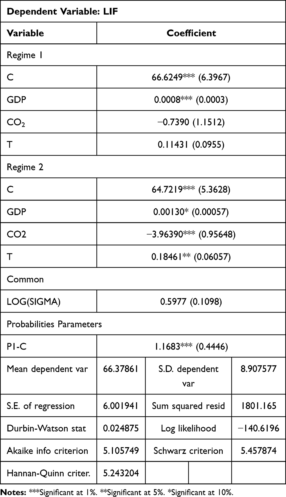Table 2 Regime Switching Regression Results

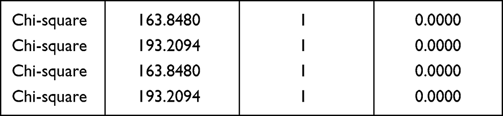Table 3 Wald Test

Diagnostic Tests

Table 3 Diagnostic Test.

Robustness Test

Table 4 reports a standard causality outcome for our baseline model. The regression model shows a one-way effect among the variables. However, there is a possibility that variables may have a bidirectional effect besides, the causality test further validates our bassline estimations. The causality test found no causality between GDP and CO₂, which implies GDP per capita does not increase CO₂ emissions. There is bidirectional causality between CO₂ causes life expectancy which supports the baseline results implying the CO₂ emissions have adverse implications on human health. There is unidirectional causality from trade openness to CO₂ emissions, which confirms our switching regression results. Besides, this implies that trade openness leads to the industrial expansion that emits a high volume of CO₂, the CO₂ and trade results are supported by past studies including Ullah et al⁷ and Ullah et al⁸ and argued that trade activities lead to CO₂ emissions due to industrial and export sector expansion. A unidirectional causality is found from GDP to life expectancy that indicates this supports our bassline findings and that per capita income causes the life expectancy. We also found a unidirectional causality from trade to GDP which implies that trade increases the per capita income in China. These findings support of theoretical model where trade openness is assumed to increase the per capita income. Finally, there we found a unidirectional causality from trade to life expectancy, which verifies our baseline regime-switching regression results and indicates that trade expansion leads to attaining a high level of life expectancy and GDP per capita is the main channel that could lead to improve the life expectancy.

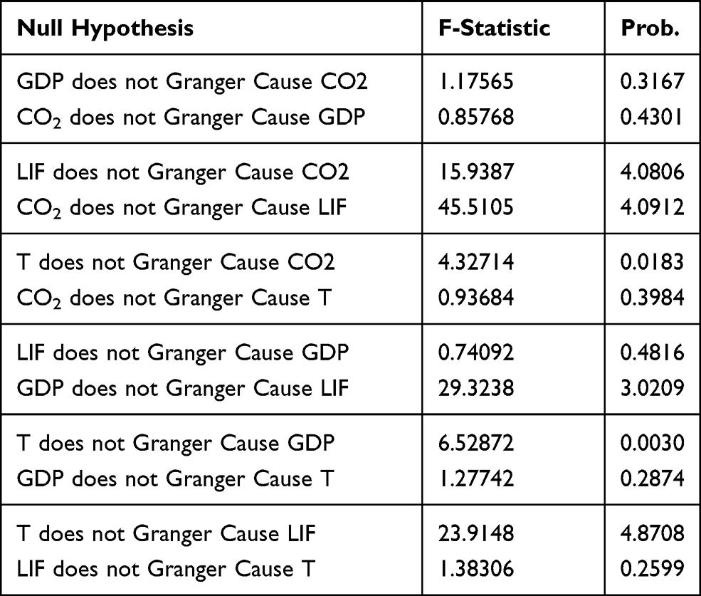Table 4 Pairwise Granger Causality Tests

Table 5 shows the trade effect on life expectancy, two separate models since our theoretical model shows that trade could affect life expectancy from two ways one is income effect and the other is the environment or CO₂ effect. This test verifies our theoretical model and further validates our baseline regime-switching regression results. Table 5 results contain two estimations; one is the net effect (income increase mins CO₂ emissions) with trade, we choose net effect as the dependent variable while trade openness as independent variables, our results show that trade has positive and significant effects on the net effect variable, this implies that trade income effect is comparatively larger than CO₂ emissions or in other words trade increases income more than CO₂ emissions. This verifies the income Granger causality test where trade causes per capita GDP and CO₂ emissions. First we found a positive net effect of trade now we test the net effect in the life expectancy model. The second estimations in Table 5 contain the results of effect variable (income effect minus CO₂ emissions) and trade on the life expectancy, we found that both trade and net effect variables have positive and significant implications for the life expectancy at 1% and 10% level of significance. This shows that life expectancy increases due to trade, and despite the increase of CO₂ emissions trade have a relatively greater income on income due to the trade expansion which resulted in a positive implication of trade for life expectancy. These results are in line with baseline regime-switching regression and granger causality outcomes. Overall our findings suggest a positive implication for the trade openness for the life expectancy from both baseline model estimation robustness tests which also in line with the theoretical model of this study.

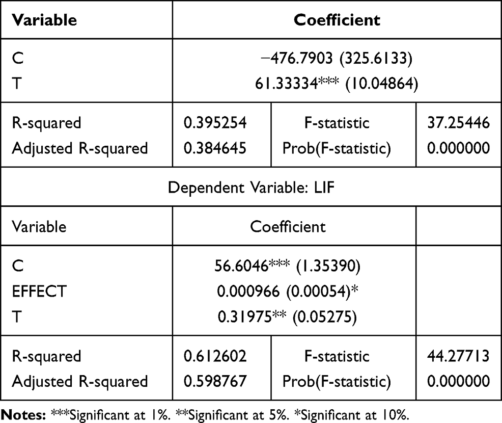Table 5 Dependent Variable: Net Effect

Conclusion

Trade liberalization has a diverse effect on the economy, environment, it improves the country’s exports, stimulates industrial production, and increases aggregate consumption. Besides the positive effect of trade, it has associated costs for society in terms of pollution particularly an increase in CO₂ emissions. Among the other pollutants, CO₂ emissions are more straightforward, the production and export expansion especially post-trade liberalization leads to CO₂ emissions, which adversely affect human health and life expectancy. Therefore, this study provides a theoretical framework for trade liberalization and life expectancy association, which is tested empirically for China using the period 1960–2018. We used regime-switching regression for the baseline model, while Granger causality and OLS with some additional specification are used as robustness tests. Our findings suggest that trade increases life expectancy, which is supported by Granger causality and OLS results. This implies that trade affects life expectancy in two ways; firstly, trade increases the overall income of the society which helps people to maintain health quality and thus improve life expectancy. Secondly, environmental degradation in the form of CO₂ emissions imposes a health cost, which leads to reduces life expectancy. The net effect of trade on life expectancy depends on the increase of both income and CO₂ emissions. Nonetheless, CO₂ emissions are the main channel through which trade liberalization could affect life expectancy. Trade activities are responsible for environmental degradation which leads to a negative implication on human health resulted in a low level of life expectancy. It is recommended that trade liberalization should be embodied with certain environmental protection policies, for example, carbon tax could mitigate the negative effect of CO₂ emissions on the economy. The adaptation of renewable energy resources along with trade liberalization policies may also offset the environmental cost of trade and improves life expectancy. Besides, the trade effect in developing and developed countries depends on the economic structure and healthcare facilities to compensate for the trade effect on human health and life expectancy.

The results derived from this study have some important policy implications. The key findings suggest that trade openness contributes to life expectancy significantly in China. Hence, the government should use trade openness as economic tools not only for enhancing domestic production but also for improving health of its massive population. Therefore, we recommend that policymakers should introduce more trade liberalization friendly policies that will ensure the maximum economic and social benefits. Moreover, foreign affiliates should largely invest in hospital and pharmaceutical sectors by bringing modern know-how and technology from their host countries which will directly benefit to the public health of the host countries.

This study has some limitations as it covers a single country which could be extended for multiple countries in the future, however, the empirical outcomes may be varied for the different countries to the difference in economic structure across the different countries.

References

1. Kohli U. Real GDP, real domestic income, and terms-of-trade changes. J Int Econ. 2004;62(1):83–106. doi:10.1016/j.jinteco.2003.07.002
2. Cutler D, Deaton A, Lleras-Muney A. The determinants of mortality. J Econ Perspect. 2006;20(3):97–120. doi:10.1257/jep.20.3.97
3. Deaton A. Relative Deprivation, Inequality, and Mortality. National Bureau of economic research; 2001:0898–2937.
4. Wagstaff A, Van Doorslaer E. Income inequality and health: what does the literature tell us? Annu Rev Public Health. 2000;21(1):543–567. doi:10.1146/annurev.publhealth.21.1.543
5. Grossman GM, Krueger AB. Environmental Impacts of a North American Free Trade Agreement. National Bureau of Economic Research; 1991:0898–2937.
6. Copeland BR, Taylor MS. Trade, growth, and the environment. J Econ Lit. 2004;42(1):7–71. doi:10.1257/.42.1.7
7. Ullah I, Ali S, Shah MH, Yasim F, Rehman A, Al-Ghazali BM. Linkages between trade, CO2 emissions and healthcare spending in China. Int J Environ Res Public Health. 2019;16(21):4298. doi:10.3390/ijerph16214298
8. Ullah I, Rehman A, Khan FU, Shah MH, Khan F. Nexus between trade, CO2 emissions, renewable energy, and health expenditure in Pakistan. Int J Health Plan Manag. 2019.
9. Yazdi S, Zahra T, Nikos M. Public healthcare expenditure and environmental quality in Iran.
10. Ostro BD, Rothschild S. Air pollution and acute respiratory morbidity: an observational study of multiple pollutants. Environ Res. 1989;50(2):238–247. doi:10.1016/S0013-9351(89)80004-0
11. Schwartz J, Dockery DW. Increased mortality in Philadelphia associated with daily air pollution concentrations. Am J Respir Crit Care Med. 1992;145(3):600–604. doi:10.1164/ajrccm/145.3.600
12. Mariani F, Pérez-Barahona A, Raffin N. Life expectancy and the environment. J Econ Dyn Control. 2010;34(4):798–815. doi:10.1016/j.jedc.2009.11.007
13. Mohmmed A, Li Z, Arowolo AO, et al. Driving factors of CO2 emissions and nexus with economic growth, development and human health in the top ten emitting countries. Resour Conserv Recycl. 2019;148:157–169. doi:10.1016/j.resconrec.2019.03.048
14. Elo IT, Preston SH. Effects of early-life conditions on adult mortality: a review. Popul Index. 1992;58(2):186–212. doi:10.2307/3644718
15. Pope C
16. Evans MF, Smith VK. Do new health conditions support mortality–air pollution effects? J Environ Econ Manag. 2005;50(3):496–518. doi:10.1016/j.jeem.2005.04.002
17. Bernard AB, Eaton J, Jensen JB, Kortum S. Plants and productivity in international trade. Am Econ Rev. 2003;93(4):1268–1290. doi:10.1257/000282803769206296
18. Fischer A. Approximation of o-minimal maps satisfying a Lipschitz condition. Ann Pure Appl Log. 2014;165(3):787–802. doi:10.1016/j.apal.2013.10.003
19. Fullerton D, Ta CL. Environmental policy on the back of an envelope: a Cobb-Douglas model is not just a teaching tool. Energy Econ. 2019;84:104447. doi:10.1016/j.eneco.2019.07.007
20. Mann DL, Kent RL, Parsons B, Cooper G
21. Mubeen S, Zhang T, Chartuprayoon N, et al. Sensitive detection of H2S using gold nanoparticle decorated single-walled carbon nanotubes. Anal Chem. 2010;82(1):250–257. doi:10.1021/ac901871d
22. Khastar M, Aslani A, Nejati M. How does carbon tax affect social welfare and emission reduction in Finland? Energy Rep. 2020;6:736–744. doi:10.1016/j.egyr.2020.03.001
23. Craig MT, Zhai H, Jaramillo P, Klima K. Trade-offs in cost and emission reductions between flexible and normal carbon capture and sequestration under carbon dioxide emission constraints. Int J Greenh Gas Control. 2017;66:25–34. doi:10.1016/j.ijggc.2017.09.003
24. Van Doorslaer E, Wagstaff A, Bleichrodt H, et al. Income-related inequalities in health: some international comparisons. J Health Econ. 1997;16(1):93–112. doi:10.1016/S0167-6296(96)00532-2
25. Ásgeirsdóttir TL, Ragnarsdóttir DÓ. Health-income inequality: the effects of the Icelandic economic collapse. Int J Equity Health. 2014;13(1):50. doi:10.1186/1475-9276-13-50
26. Shapiro JS. Trade costs, CO 2, and the environment. Am Econ J. 2016;8(4):220–254.
27. Chaabouni S, Saidi K. The dynamic links between carbon dioxide (CO2) emissions, health spending and GDP growth: a Case Study for 51 countries. Environ Res. 2017;158:137–144. doi:10.1016/j.envres.2017.05.041
28. Chaabouni S, Zghidi N, Mbarek MB. On the causal dynamics between CO2 emissions, health expenditures and economic growth. Sustain Cities Soc. 2016;22:184–191. doi:10.1016/j.scs.2016.02.001
29. de Koeijer G, Talstad VR, Nepstad S, et al. Health risk analysis for emissions to air from CO2 technology centre mongstad. Int J Greenh Gas Control. 2013;18:200–207. doi:10.1016/j.ijggc.2013.07.010
30. Shaw JW, Horrace WC, Vogel RJ. The determinants of life expectancy: an analysis of the OECD health data. South Econ J. 2005;71(4):768–783. doi:10.2307/20062079
31. Dobis EA, Stephens HM, Skidmore M, Goetz SJ. Explaining the spatial variation in American life expectancy. Soc Sci Med. 2020;246:112759. doi:10.1016/j.socscimed.2019.112759
32. Huebener M. Life expectancy and parental education. Soc Sci Med. 2019;232:351–365. doi:10.1016/j.socscimed.2019.04.034
33. Agnisarman S, Ponathil A, Lopes S, Madathil KC. An investigation of consumer’s choice of a healthcare facility when user-generated anecdotal information is integrated into healthcare public reports. Int J Ind Ergon. 2018;66:206–220. doi:10.1016/j.ergon.2018.03.003
34. Malafarina V, Rexach JAS, Masanes F, Cruz-Jentoft AJ. Effects of high-protein, high-calorie oral nutritional supplementation in malnourished older people in nursing homes: an observational, multi-center, prospective study (PROT-e-GER). Protocol and baseline population characteristics. Maturitas. 2019;126:73–79. doi:10.1016/j.maturitas.2019.05.009
35. Kabir M. Determinants of life expectancy in developing countries. J Dev Areas. 2008;41(2):185–204. doi:10.1353/jda.2008.0013
36. Chen B, Feng Y. Openness and trade policy in China: an industrial analysis. Chin Econ Rev. 2001;11(4):323–341. doi:10.1016/S1043-951X(01)00034-7
37. Ji JS, Zhu A, Lv Y, Shi X. Interaction between residential greenness and air pollution mortality: analysis of the Chinese longitudinal healthy longevity survey. Lancet Planet Health. 2020;4(3):e107–e115. doi:10.1016/S2542-5196(20)30027-9
38. Wu Y, Wang W, Liu C, Chen R, Kan H. The association between long-term fine particulate air pollution and life expectancy in China, 2013 to 2017. Sci Total Environ. 2020;712:136507. doi:10.1016/j.scitotenv.2020.136507
39. Goldfeld S, Quandt R. The estimation of structural shifts by switching regressions. Ann Econ Soc Meas. 1973;2(4):475–485. NBER.
40. Maddala GS. Disequilibrium, self-selection, and switching models. Handb Econ. 1986;3:1633–1688.
41. Hamilton JD, Susmel R. Autoregressive conditional heteroskedasticity and changes in regime. J Econom. 1994;64(1–2):307–333. doi:10.1016/0304-4076(94)90067-1
42. Frühwirth-Schnatter S. Finite Mixture and Markov Switching Models. Springer Science & Business Media; 2006.
43. Weixiang L, Yu X. Economic growth, income inequality and life expectancy in China. Soc Sci Med. 2020;113046.
44. Hansen AC, Selte HK. Air pollution and sick-leaves. Environ Resour Econ. 2000;16(1):31–50. doi:10.1023/A:1008318004154
45. Apergis N, Gupta R, Lau CKM, Mukherjee Z. US state-level carbon dioxide emissions: does it affect health care expenditure? Renew Sustain Energy Rev. 2018;91:521–530. doi:10.1016/j.rser.2018.03.035
46. Zeeshan M, Han J, Alam rehman HB, et al. Nexus between foreign direct investment, energy consumption, natural resource, and economic growth in Latin American countries. Int J Energy Econ Policy. 2021;11(1):407–416. doi:10.32479/ijeep.10255
© 2021 The Author(s). This work is published and licensed by Dove Medical Press Limited. The
full terms of this license are available at https://www.dovepress.com/terms
and incorporate the Creative Commons Attribution
- Non Commercial (unported, 3.0) License.
By accessing the work you hereby accept the Terms. Non-commercial uses of the work are permitted
without any further permission from Dove Medical Press Limited, provided the work is properly
attributed. For permission for commercial use of this work, please see paragraphs 4.2 and 5 of our Terms.