Localization for robotic capsule looped by axially magnetized permanent-magnet ring based on hybrid strategy

Introduction

Wireless capsule endoscopy (WCE), a significant cableless technique, provides painless and friendly inspection of the whole gastrointestinal (GI) tract.^1–4 WCE integrates a microcamera and illuminating system for taking photos, and sends them wirelessly to a receiver outside the human body.

Accurate positioning and orientation of the capsule when it moves in the GI tract are essential for the doctor to determine where the diseases are located. The efficacy of drug release and further therapeutic operations also depend heavily on the accuracy of the positional and orientation information.⁵ Therefore, a precise and reliable localization system plays an important role in enhancing the benefits of WCE.

Magnetic localization methods have attracted the attention of researchers for two main reasons.^6,7 Firstly, magnetic localization is a non-line-of-sight method in which the capsule does not need to be in the line of sight with magnetic sensors outside the body in order to be detected. Secondly, magnetic signals produced by the magnet can pass through human tissue without attenuation.

Many scholars have conducted work related to magnetic localization. Weitschies et al adopted such a technique for monitoring the transit of a capsule in the GI tract.^8,9 The magnetic marker monitoring utilized a superconducting quantum-interference sensor system with 37 channels above a volunteer’s abdomen. It was reported that the position resolution was within a range of millimeters in a magnetically shielded room. Schlageter et al also introduced an approach that used a 2-D array of 16 hall sensors to determine the position and orientation of a pill-size magnet coated with silicone.^10,11 Wu et al exploited a wearable magnetic locating system that allows patients to move with different postures during diagnostic process.¹² The magnetic signals originating from a small (diameter 5 mm × length 3 mm) cylindrical magnet embedded inside the capsule. In our previous research, we developed a 50×50×50 cm cubic sensor array.⁷ This cubic sensor array is formed by two pairs of sensor planes. The system can achieve about an average position error of 2 mm and orientation error of 2°.

From previous research about magnetic localization techniques, it may be found that it is feasible to localize WCE by using magnetic techniques. However, lack of localization function is the main problem of the current guidance system. For example, Swain et al tested a new capsule-manipulation system in a volunteer. One imager of WCE was removed from the PillCam colon-based capsule, and the available space was used to house the magnets. An Olympus GIF 180 high-definition videogastroscope was used to observe the capsule in the esophagus and stomach. The system did not integrate with a localization unit.¹³ Rey et al magnetically navigated a capsule in the human stomach. The prototype included an Olympus capsule endoscope and Siemens magnetic guidance equipment for interactively moving the capsule in the gastric cavity. Real-time gastric-imaging sensors were used to observe maneuvers and settings for moving the capsule.¹⁴ The function of positioning the capsule was not achieved. Keller et al also reported a similar guiding system in which the outer magnetic fields are produced by complex electromagnetic coils.¹⁵ The system did not include a localization function. If the guidance system is integrated with a magnetic localization unit, diagnosis may benefit more.

The Given Imaging PillCam is 11 mm in diameter and 26 mm long.¹⁶ All its components, such as circuits, imaging device, and batteries, are assembled inside the capsule. Expansion of the capsule would make it hard to swallow. Therefore, we suggest that the capsule is looped by a thin permanent-magnet ring (a mimic capsule is shown in Figure 1), which only increases the dimensions of the capsule a little. However, the magnetic field distribution of the magnet ring is different from a cylindrical magnet (regarded as a dipole), so localization for a magnet ring needs further investigation.

Figure 1 The mimic robotic capsule.

The paper is organized as follows. In the following sections, we introduce the localization method, present the localization model based on the magnet ring’s magnetic field, propose algorithms and show simulation results, and finally draw conclusions.

Localization schema

The capsule is looped by a permanent magnet ring with 18 mm length, 4.5 mm inner radius, and 5.5 mm outer radius. In the “Algorithms and experimental results” section, the parameters of the magnet ring are equal to these values. As shown in Figure 2, the magnet ring generates magnetic fields around the human body whose intensities are determined by the position and orientation of the magnet ring, which is different from a cylindrical magnet (regarded as a dipole). We built a mathematical model for this magnet ring’s field, and emulated a 64-magnetic-sensor array that measures the magnetic intensities in some spatial points around the human body. These measured magnetic field data can be used to seek the magnet ring’s position and orientation parameters through an appropriate algorithm, which solves the high-order nonlinear localization model related to the magnet’s fields. In the simulation experiment, the measured data were replaced by calculated values that come from the expressions of magnetic fields of the magnet ring.

Figure 2 Localization schema.

Localization model of the magnet ring

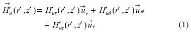
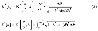
The geometry and parameters of the permanent-magnet ring are shown in Figure 3. The inner radius of the ring is r_in, the outer radius r_out, and the height h. The upper plane is charged with a surface magnetic pole density +σ*; the lower plane is charged with the opposite surface magnetic pole density −σ* (+σ*and −σ* are constants once the magnetic ring is selected). 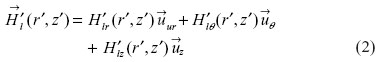The magnetic field created by the upper plane of the ring at any observation point P(r′, z′) of space is given by Equation 1,¹⁷ and the magnetic field created by the lower plane of the ring at the same point is given by Equation 2:

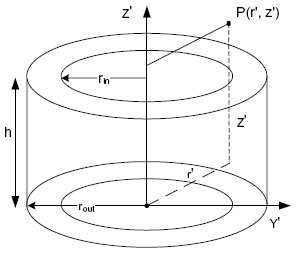Figure 3 Geometry of the ring with axial magnetic polarization.

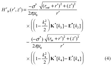
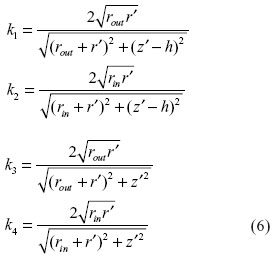
where , and are components along the three directions , and . The upper and lower radial components are represented by Equations 3 and 4, respectively, where u₀ is the air magnetic permeability (T · m/A):

with

The upper and lower azimuthal components and are equal to zero on account of the cylindrical symmetry. The axial components and should be real numbers; however they contain the imaginary number i (i²=−1) (the real expressions have not been obtained), so in the localization only the radial components and can be used. The total radial component of the magnet ring is given by Equation 7:

We call the coordinate system in Figure 3 the local coordinate system (O′, X′, Y′, Z′). In the localization process, the local coordinate system actually moves along with the magnet ring’s movement, so the position and orientation of the magnet ring cannot be expressed by the local coordinate system. Another stationary global coordinate system (O, X, Y, Z), together with the local coordinate system, should be established to realize localization for the magnet ring. Figure 4 shows the two coordinate systems.

Figure 4 Global and local coordinate systems.

(O, X, Y, Z) is the stationary global coordinate system, (r, z) is the global coordinate of point P, and (r′, z′) is the local coordinate of the same point P. To simplify description for the position of the magnet ring, the origin of the local coordinate system with respect to the global coordinate system is regarded as the position of the magnet ring. In fact, if the coordinate of the origin of the local system is obtained, the position of the magnet ring’s center with respect to the global coordinate system can be calculated through rotation and translation transform.

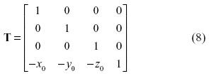
In order to express the translation relationship of a point in a two-coordinate system, the translation transform matrix is defined in Equation 8. (x₀, y₀, z₀) is the coordinate of the origin O' of the local coordinate system with respect to the global coordinate system.

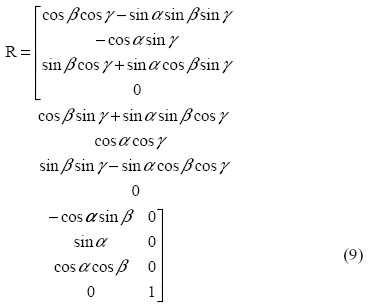
The magnet ring’s orientation can be represented by Euler angles.^18,19 The rotation matrix containing Euler angles is defined in Equation 9, where α, β, and γ are pitch, yaw, and roll, respectively, and α is in [−180°, 180°], β is in [−90°, 90°], and γ is in [−180°, 180°]. When doing rotation transform, firstly rotate around the Y′-axis (yaw), then rotate around the X′-axis (pitch), and finally rotate around the Z′-axis (roll). The global coordinate (x, y, z) and the local coordinate (x′, y′, z′) of any point in the space satisfy Equation 10.

Equation (10) can be further rewritten as Equations 11, 12, and 13:

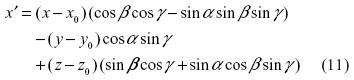
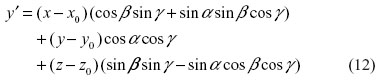
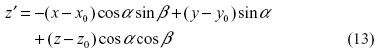
The global position parameters x, y, z, related to the position of the magnetic sensor, are known in advance; x', y', and z' are functions of the unknown parameters x₀, y₀, z₀, α, β, γ. Substituting Equations 11, 12, and 13 into 3, 4, 7, and 14, we get the theoretic global value of H_r that is the function of the unknown parameters x₀, y₀, z₀, α, β, γ.

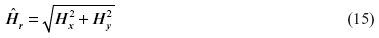
A three-axis magnetic sensor can measure three global magnetic fields: H_x, H_y, and H_z. In the localization process, only the magnetic fields H_x and H_y are used. According to Equation 15, the measured global value can be obtained.

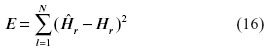
Assume that there are n three-axis sensors, with the l-th sensor located at point P_l (1 < l ≤ n), for each sensing point, magnetic fields H_x, H_y, and H_z are measured; and for n sensors, n-measured radial components are obtained. With at least six three-axis magnetic sensors, the localization and orientation parameters of the magnetic ring can be calculated by minimizing E defined by Equation 16, where is the measured value, and H_r is the theoretic value:

Algorithms and experimental results

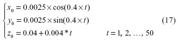
Before evaluating the performance of the algorithm, sample points should be determined. In the following experiments, the points are sampled along the locus that is represented in Equation 17:

In order to evaluate the convergence and accuracy of the algorithm, the localization error E_p and orientation error E_o are defined by Equations 18 and 19, where x_c, y_c, z_c, α_c, β_c, and γ_c are calculated values for x₀, y₀, z₀, α, β, and γ, and x_t, y_t, z_t, α_t, β_t, and γ_t are true values for x₀, y₀, z₀, α, β, and γ:

Performance of TRR, LM, and PSO algorithms

The size of the sensor space will influence the accuracy of algorithm. Considering real application in the future, 64 sensors distributed symmetrically on the cubic space 0.5×0.5×0.5 m were used to sample data. This sensor space is suitable for most people. The following experiments follow this configuration.

Minimizing E of Equation 16 is a least-square problem that can be solved by an optimization algorithm. Considering a real-time request and high efficiency of the gradient-descent-optimization algorithm, we first evaluated the performance of the trust-region-reflective (TRR) and Levenberg–Marquardt (LM) algorithms to solve the localization model. The tolerance of initial guess error, convergence, and execution time are important aspects that we care about. Table 1 lists the localization results.

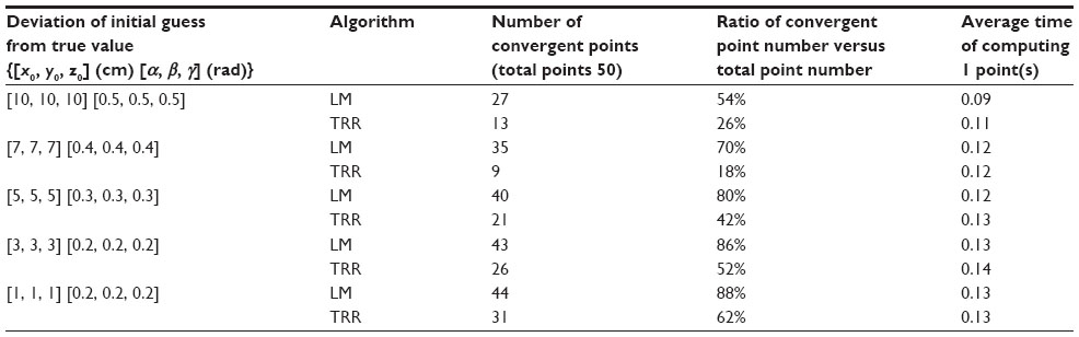Table 1 Localization results by TRR and LM algorithms Abbreviations: LM, Levenberg–Marquardt; TRR, trust-region-reflective.

From Table 1, we can draw three conclusions. First, convergences of both LM and TRR increase with decrease of initial guess error. Second, convergence of LM is better than TRR whatever the initial guess errors are. Third, the execution time has little difference.

However, the real initial position and orientation of the capsule is unknown in the real localization process, and a better initial guess is difficult to give. If the initial guess error is large, the gradient-descent algorithm may be divergent. Therefore, the initial-guess problem should be solved. The evolution algorithm particle-swarm optimization (PSO) does not require an initial guess. This algorithm starts to work as long as the ranges of all the parameters are given. This advantage is just what we want, in that the position of the capsule is in 0.5 m³, and the Euler angles are also restricted in scope. Therefore, the performance of the standard PSO algorithm is investigated for solving the localization model.

Assume D to be the dimension of the solution space, and n the population size, the ith particle is X_i = (x_i1, x_i2, …, x_iD) (1 ≤ i ≤ n). The previous best position of the ith particle is Pi = (p_i1, p_i2, …, p_iD); the index of the best position of particles in the whole group is g, and the flight velocity is Δxi = (Δx_i1, Δx_i2, …, Δx_iD). For each evolution step, all the particles update themselves as per the following two equations:

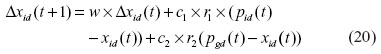
Here, c₁, c₂, adjusting the weight of a single particle’s experience and group particles’ experiences, are called acceleration constants, w is inertia-weight constant, and r₁ and r₂ are random numbers in [0, 1]. The fitness function for the PSO algorithm is E defined by Equation 16.

In the evolution process, the maximum iterative number is 25, and the population number is 100. As shown in Figures 5 and 6, the average localization error reaches 10.8 cm, and the average orientation is 0.29 rad. If this value is treated as the initial guess of the LM algorithm, the convergence probability of the LM algorithm is about 54% according to Table 1. The average localization error is expected to be less than 1 cm.^20,21 Therefore, the accuracy of the standard PSO algorithm cannot meet the localization requirement. In the following section, we provide the enhanced PSO algorithm.

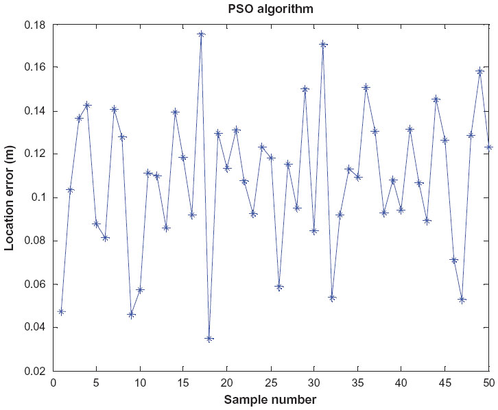Figure 5 Localization error of the particle-swarm optimization (PSO) algorithm.

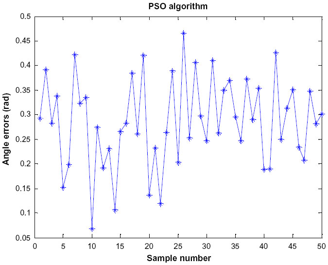Figure 6 Orientation errors of the particle-swarm optimization (PSO) algorithm.

Performance of a hybrid strategy: combined PSO and clone algorithms

The PSO algorithm has a good ability to search global optimal solutions. However, it sometimes falls into local minimum point. The clone algorithm has strong local searching ability by producing a new subgroup whose population number is proportional to the fitness of the particle, and maintaining population diversity by reinitializing particles that have low fitness. In the iterative process of the clone algorithm, however, the particles cannot share information with each other because they mutate randomly. To utilize the advantages of both the PSO and clone algorithms, we introduced the evolutionary equation of the PSO algorithm into the clone algorithm. Because the particles have utilized their previous individual optimization information in the clone algorithm, only global optimization information is considered in the PSO algorithm. Therefore, in the hybrid strategy, all the particles update by using Equations 20 and 22.

The steps of the hybrid strategy are as follows:

1. initialize particle original position and flight velocity
2. compute all the particles’ fitness according to Equation 16
3. check whether the algorithm should stop
4. update all the particles according to Equations 21 and 22.
5. put k particles with best fitness into subset Am
6. produce new clone subset Ac by cloning every particle of group Am; the clone number n_c of each particle is inversely proportional to its fitness (here, it is a minimization problem; if it is a maximization problem, the clone number is proportional to the particle’s fitness)
7. mutate every particle of Ac (the mutation ratio β is inversely proportional to its fitness)
8. recompute every particle’s fitness in clone subset Ac
9. if there exists a particle p_c in subset Ac whose parent is p_r, (f (p_c) < f (p_r), f is objective function), substitute p_c for p_r, and update global optimization particle p_g
10. return to step 3.

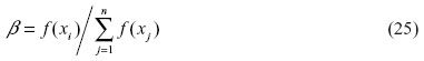
In step 6, the clone number n_c is calculated by Equation 23. Where α is a clone constant whose value is in (0, 1), and n is the population number, i is the sequence number of the particle (the particles are sorted according to their objective function value, from smallest to biggest).

In the evolution, to ensure the particles with lower fitness have lower mutation probability (this is a minimum problem; if it is a maximum problem, the particles with lower fitness have higher mutation probability), and to keep diversity of the particles, a self-adapted mutation operator is adopted, as shown in Equations 24 and 25,²² where n (0, 1) is a random number obeying the law of standardized norm distribution:

To compare with the PSO algorithm, the same 64 sensors are used, and the sample points are completely identical. The maximum iterative number is 25; the population number is 100. The localization and orientation errors are shown in Figures 7 and 8. The average localization error is about 0.9 mm; the average orientation error is about 0.12 rad. The execution time is shown in figure 9, which range is from 4.95 to 5.75. The average time is about 5.15, which seems to be a little longer from the point of real time performance. Compared with the standard PSO algorithm, the localization and orientation accuracies of the hybrid algorithm are improved greatly. However, the solutions do not converge completely. If the result of the hybrid algorithm is regarded as the initial guess of the LM algorithm, the convergence probability will be over 88%. Compared with the LM algorithm, the time consuming of one point is 5 seconds, which shows that the hybrid strategy of the PSO and clone algorithms cannot be used as the final strategy to track the capsule, so we find the final strategy that has real time performance and good convergence.

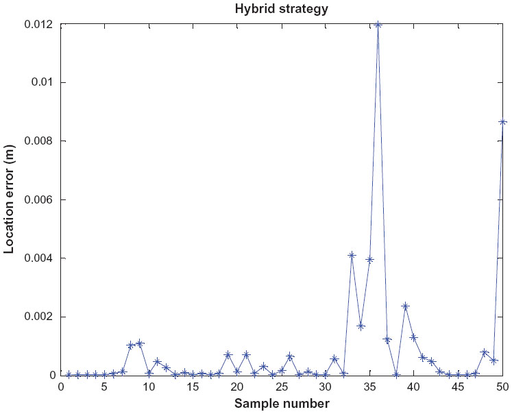Figure 7 Localization errors of the hybrid strategy.

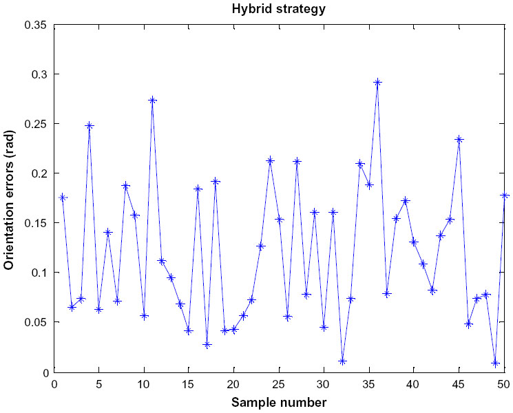Figure 8 Orientation errors of the hybrid strategy.

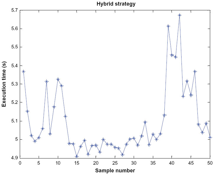Figure 9 Execution time of the hybrid strategy.

Final strategy

From the experiments in previous sections, it can be found that the LM algorithm has high efficiency compared with the standard PSO or hybrid algorithm. The LM algorithm has stronger initial guess-error toleration and convergence compared with the TRR algorithm. The hybrid strategy of the PSO and clone algorithms has better accuracy compared with the standard PSO algorithm, and it does not need an initial guess compared with the LM algorithm. With better accuracy, initial guess, and high efficiency, the final strategy is determined. First, compute the initial point of the capsule in the cubic space 0.5×0.5×0.5 m by the hybrid strategy of combined PSO and clone algorithms. Then, compute the second point by the LM algorithm which initial guess comes from the first point value. Third, the following tracking uses the LM algorithm which initial guess is previous point value. After using this strategy, only first-point computation requires more time, but it provides a better initial guess for second-point computation, which ensures the convergence and real time. Figures 10 and 11 show the localization and orientation error in a tracking process. The localization and orientation errors of each point are very close to zero, which shows that the 50 points are convergent. However, sometimes not all points are convergent; the reason is that the initial guess of the first point computed by the hybrid strategy is far from the true value. Table 2 lists the convergent times per ten times. The convergent probability is about 90%. One-point computation time is about 0.1 seconds except the first point, which is the same as the efficiency of the LM algorithm.

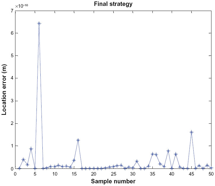Figure 10 Localization errors of the final strategy.

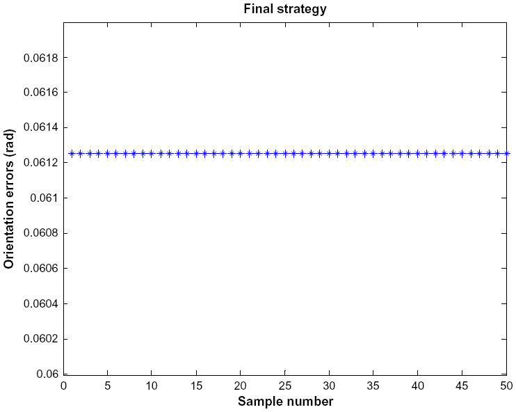Figure 11 Orientation errors of the final strategy.

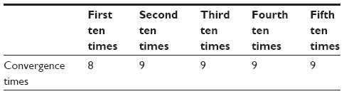Table 2 Convergence of the final strategy

Conclusion

Permanent magnets have attracted many scholars’ attentions in recent years, thanks to the advantages of magnetic fields. Magnetic localization for WCE is one example, and one common feature of the permanent-magnet-based localization schema is to enclose the cylindrical magnet in the capsule. One problem is that the dimensions of the robotic capsule are limited. If an extra magnet is added, the expansion of the capsule’s dimensions would make it hard to swallow. To address this limitation, we suggest that the capsule is looped by a thin permanent-magnet ring. However, the distribution of the magnetic field is different from that of the cylindrical magnet (simplified magnetic dipole), so based on the radial component of the magnetic field of the magnet ring, we establish the localization model of axially magnetized magnet ring. With regard to accuracy, initial guess, and time efficiency, an appropriate hybrid strategy for seeking the position and orientation of the magnet ring is developed. Experimental results show that the strategy has good convergence, stability, and real time performance.

Acknowledgments

This project was supported by the National Natural Science Foundation of China (grants 61202196, 61273332, and 61202195), the China Scholarship Council, Scientific Research Fund of the Sichuan Provincial Education Department (grant 12ZA200), the Yibin Scientific and Technological Project (grant 2013ZSF010), and the Doctoral Fund of Yibin University (grant 2011B06).

Disclosure

The authors report no conflicts of interest in this work.

---

References

1.	Iddan G, Meron G, Glukhovsky A, Swain P. Wireless capsule endoscopy. Nature. 2000;405(6785):417.
2.	Than TD, Alici G, Zhou H, Li W. A review of localization systems for robotic endoscopic capsules. IEEE Trans Biomed Eng. 2012;59(9):2387–2399.
3.	Glukhovsky A. Wireless capsule endoscopy. Sens Rev. 2003;23(2):128–133.
4.	Moglia A, Menciassi A, Dario P, Cuschieri A. Capsule endoscopy: progress update and challenges ahead. Nat Rev Gastroenterol Hepatol. 2009;6(6):352–362.
5.	Toennies JL, Tortora G, Simi M, Valdastri P, Webster RJ. Swallowable medical devices for diagnosis and surgery: the state of the art. Proc Inst Mech Eng C J Mech E. 2010;224(7):1397–1414.
6.	Atuegwu NC, Galloway RL. Volumetric characterization of the aurora magnetic tracker system for image-guided transorbital endoscopic procedures. Phys Med Biol. 2008;53(16):4355–4368.
7.	Chao H, Mao L, Shuang S, Wan’an Y, Rui Z, Meng MQ. A cubic 3-axis magnetic sensor array for wirelessly tracking magnet position and orientation. IEEE Sens J. 2010;10(5):903–913.
8.	Weitschies W, Kötitz R, Cordini D, Trahms L. High-resolution monitoring of the gastrointestinal transit of a magnetically marked capsule. J Pharm Sci. 1997;86(11):1218–1222.
9.	Weitschies W, Wedemeyer J, Stehr R, Trahms L. Magnetic markers as a noninvasive tool to monitor gastrointestinal transit. IEEE Trans Biomed Eng. 1994;41(2):192–195.
10.	Schlageter V, Besse PA, Popovic RS, Kucera P. Tracking system with five degrees of freedom using a 2D-array of hall sensors and a permanent magnet. Sens Actuators A Phys. 2001;92(1–3):37–42.
11.	Schlageter V, Drljaca P, Popovic RS, Kučera P. A magnetic tracking system based on highly sensitive integrated hall sensors. JSME Int J Ser C. 2002;45(4):967–973.
12.	Wu X, Hou W, Peng C, Zheng X, Fang X, He J. Wearable magnetic locating and tracking system for MEMS medical capsule. Sens Actuators A Phys. 2008;141(2):432–439.
13.	Swain P, Toor A, Volke F, et al. Remote magnetic manipulation of a wireless capsule endoscope in the esophagus and stomach of humans. Gastrointest Endosc. 2010;71(7):1290–1293.
14.	Rey JF, Ogata H, Hosoe N, et al. Feasibility of stomach exploration with a guided capsule endoscope. Endoscopy. 2010;42(7):541–545.
15.	Keller H, Juloski A, Kawano H, et al. Method for navigation and control of a magnetically guided capsule endoscope in the human stomach. Poster presented at: Biomedical Robotics and Biomechatronics, 4th IEEE RAS and EMBS International Conference; June 24–27, 2012; Rome, Italy.
16.	Sidhu R, Sanders DS, McAlindon ME. Gastrointestinal capsule endoscopy: from tertiary centres to primary care. BMJ. 2006; 332(7540):528–531.
17.	Ravaud R, Lemarquand G, Lemarquand V, Depollier C. Analytical calculation of the magnetic field created by permanent-magnet rings. IEEE Trans Magn. 2008;44(8):1982–1989.
18.	Pio RL. Euler angle transformations. IEEE Trans Automat Contr. 1996;11(4):707–715.
19.	Diebel J. Representing attitude: Euler angles, unit quaternions, and rotation vectors. 2006. Available from: http://www.astro.rug.nl/software/kapteyn/_downloads/attitude.pdf. Accessed December 29, 2014.
20.	Chao H. Localization and Orientation System for Robotic Wireless Capsule Endoscope [doctoral thesis]. Edmonton: University of Alberta; 2006.
21.	Chao H, Meng MQ, Mrinal M. A linear algorithm for tracing magnet’s position and orientation by using 3-axis magnetic sensors. IEEE Trans Magn. 2007;43(12):4096–4101.
22.	Lijue L, Zixing C, Jin T. Immunity clone algorithm with particle swarm optimization. J Comput Appl. 2006;26(4):886–887.