Back to Archived Journals » Energy and Emission Control Technologies » Volume 2
In-depth review of atmospheric mercury: sources, transformations, and potential sinks
Received 18 March 2014
Accepted for publication 13 May 2014
Published 6 August 2014 Volume 2014:2 Pages 1—21
DOI https://doi.org/10.2147/EECT.S37038
Checked for plagiarism Yes
Review by Single anonymous peer review
Peer reviewer comments 2
Video abstract presented by Jeffrey S Gaffney
Views: 788
Jeffrey S Gaffney, Nancy A Marley
Department of Chemistry, University of Arkansas at Little Rock, Little Rock, AK, USA
Abstract: Mercury is a toxic heavy metal that is found naturally throughout the global environment. During the last 100 years, there has been a 70% rise in atmospheric mercury levels over the natural background measured prior to industrialization due to anthropogenic emissions. This increase in mercury levels represents a global threat to the health of ecosystems and humans worldwide. Atmospheric mercury chemistry is complex and its sources and sinks involve equilibrium interactions between the atmosphere, the hydrosphere, and the geosphere. This review outlines the fundamental chemistry of mercury in gas, aqueous, and solid phases, including inorganic, organic, and complexed mercury species. An understanding of this chemistry is important for understanding the cycling between the various environmental compartments as it affects atmospheric loadings. Further, many of these reactions can also occur in the atmosphere in heterogeneous gas/cloud/aerosol interactions. The sources and fate of mercury in the atmosphere, including the cycling of mercury through soil and water as it impacts atmospheric loadings are therefore examined. The sources of major uncertainties in our understanding of mercury in the atmosphere are also discussed, along with recommendations for future studies that include both homogeneous and heterogeneous reactions of the various mercury species.
Keywords: atmospheric mercury, mercury emission sources, mercury reactions, mercury speciation, atmospheric removal
Introduction
Mercury is a naturally occurring toxic heavy metal that is found everywhere throughout the environment. It exists naturally in many minerals, including cinnabar (HgS), corderoite (Hg3S2Cl2), and livingstonite (HgSb4S8). Cinnabar, the most common mercury ore, is usually found associated with recent volcanic activity and alkaline hot springs. However, mercury also occurs as an impurity in nonferrous metals and fossil fuels, coal in particular. Mercury is transported throughout the global environment after being released from these geological reservoirs by either natural or anthropogenic processes. After release, it cycles between the atmosphere, land, and surface waters through a complex web of physical and chemical transformations that have a dramatic effect on its chemical properties, environmental impacts, and biological toxicity.
Although the primary mode of global transport for mercury is by way of the atmosphere, the environmental and health impacts of mercury are not directly related to its atmospheric loadings.1 Instead, it is deposited from the atmosphere by various processes into terrestrial and aquatic systems. Once deposited, it can be transformed and bioaccumulated in the aquatic food web or it can be resuspended and re-emitted back into the atmosphere for further transport and redeposition. Although it is bioaccumulation in the aquatic environment that represents the primary route of exposure for humans and wildlife, the cycle of deposition and resuspension is also important in that it allows mercury to be transported long distances from the source.2 In addition, the different chemical species of mercury have dramatically different chemical properties and reactivities in each of the environmental compartments, not all of which are completely understood. These chemical differences affect the residence times and biological toxicities of the different mercury species. Hence, the complex factors that control the atmospheric transport and deposition, chemical speciation, re-emission, and eventual bioaccumulation of mercury also control the ecosystem impacts and the human exposure threat. It is thus impossible to assess the overall impacts of this toxic metal in the atmosphere without understanding the chemical and physical properties and transformations in each of the environmental compartments. It is for this reason that this review of atmospheric mercury will also include discussions of the chemical and physical transformations in soil and water as they impact atmospheric loadings as well as the toxicity and overall environmental impacts of this important heavy metal.
Chemistry of mercury
Elemental mercury (Hg0) is a heavy silvery fluid and the only metal that is a liquid at ambient temperatures. Mercury has one of the narrowest liquid state temperature ranges of any metal, with a freezing point of −39°C and a boiling point of 357°C. It is commonly known as quicksilver and was formerly named hydrargyrum, from the Greek “hydr-” (water) and “argyros” (silver). It is from this ancient name that it derives its atomic symbol (Hg). Mercury has a unique electronic configuration that is responsible for its anomalous chemical properties. With an atomic number of 80, the electrons fill up all the available electronic subshells through 6s (1s2, 2s2p6, 3s2p6d10, 4s2p6d10f14, 5s2p6d10, and 6s2). The ground state configuration is therefore spherically symmetric (1S0) with a very low polarizability, which strongly resists the removal of an electron, giving mercury a very high ionization potential. Mercury is thus more difficult to oxidize than other heavy metals. Since all the principal energy levels are completely filled, the chemical behavior of mercury is similar to that of the noble gases in that it forms only weak bonds and the solid form melts easily at relatively low temperatures when compared with other heavy metals. Mercury can combine with other metals to form amalgams, but the metal–metal bonding is very weak due to the fact that the mercury valence electrons are not readily shared. In fact, mercury is the only metal that does not exist as a dimer in the gas phase.3
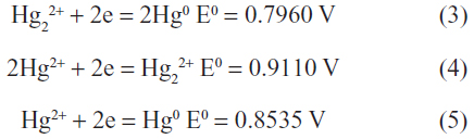
Since the mercury–mercury bonds are very weak, elemental mercury is more volatile than any other metal, with a vapor pressure of 0.261 Pa (2.58×10⁻⁶ atm) at 25°C. The vapor pressure increases logarithmically with temperature as shown in Figure 1 and doubles with every 10 degree increase.4,5 Mercury is slightly soluble in water, with a solubility of 59 μg/L at 25°C and a logarithmic temperature dependence shown in Figure 2.6 The solubility of mercury in water increases by a factor of approximately 1.3 for every 10 degree rise in temperature. The Henry’s law constant for elemental mercury, expressed as the ratio of the partial pressure above the solution to the solution concentration (KH = PHg/caq), is 8.7×10⁻³ atm-m3/mol at 25°C.6 For comparison, this value is similar to that of ethylbenzene at 7.9×10³ atm-m3/mol at 25°C.7 The temperature dependence of the Henry’s law constant shown in Figure 3 increases by about a factor of 1.6 for every 10 degree temperature rise.6
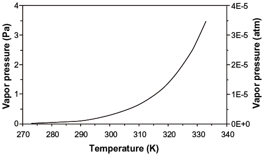 | Figure 1 Vapor pressure of elemental mercury as a function of temperature. |
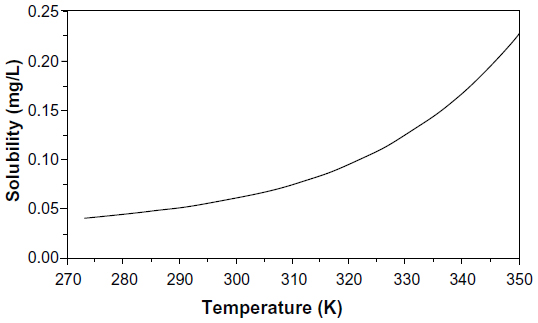 | Figure 2 Solubility of elemental mercury in water as a function of temperature. |
 | Figure 3 Henry’s law constant as a function of temperature for elemental mercury in water. |
Mercury occurs naturally in two oxidation states, ie, mercury(I), which exists as the dimeric cation (Hg22+), formerly called the mercurous ion, and mercury(II) (Hg2+), also called the mercuric ion. Mercury(I), rapidly and reversibly disproportionates to give elemental mercury and mercury(II), as:

The disproportionation constant for equation (1):
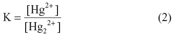
is equal to 1.14×10⁻² at an ionic strength of zero and 6.9×10⁻³ at an ionic strength of 0.7 typical of seawater.8 This implies that Hg22+ is stable by only a small margin under most environmental conditions, and any species that stabilizes Hg2+ by complexation or precipitation will increase the disproportionation of Hg22+. Since there are many such species in the environment, there are few naturally found stable compounds of Hg22+.9
The standard reduction potentials for the mercury ions are:10
Hence, only oxidizing agents with potentials in the narrow range of –0.80 V to –0.85 V are able to oxidize Hg0 to Hg22+.8 Since there are no natural oxidizing agents that fall in this narrow range, the oxidation of elemental mercury in the environment will form Hg2+. However, when Hg0 is in excess, it readily reduces Hg2+ to Hg22+ according to equation (1) and the Hg22+ can thus be observed.
The solubilities reported for some relevant mercury compounds are given in Table 1.8,11–14 It should be noted, however, that the aquatic mercury salt systems are very complex due to the competing reactions in natural aquatic environments, including: the disproportionation equilibrium, the tendency of mercury salts to hydrolyze under certain conditions of pH and temperature, the tendency of the mercury cations to form stable complexes, the acid-base nature of the mercury cations and of the appropriate counter ions, and the activity effects due to varying ionic strengths.8 It is therefore difficult to model the complex behavior of mercury and mercury salts in aqueous electrolyte solutions of environmental relevance, and this has sometimes led to wide ranging estimates of the solubilities. In addition, many laboratory investigations have reported problems achieving mass balance in mercury solubility studies, which was attributed to the air oxidation of mercury.8 The data reported in Table 1 should therefore be considered as the best estimates at this time.
 | Table 1 Physical and chemical properties of mercury and some of its compounds at 20°C–25°C |
Mercury(I) forms a linear covalent compound with the all the halides except fluorine, with the structure X-Hg-Hg-X. The most important mercury(I) compound with respect to the environment is the chloride (Hg2Cl2), with a water solubility of 4 mg/L. Mercury(I) forms very few coordination complexes in aqueous systems. This is partially due to the low tendency of Hg22+ to form covalent bonds, but also due to the much higher reactivity of mercury(II) towards most ligands. The smaller Hg2+ ion is a much better electron acceptor than the larger Hg22+ ion which favors the formation of mercury(II) complexes and the disproportionation of mercury(I).10
Oxygen-containing ligands that form ionic metal-ligand bonds can form stable ionic complexes with mercury(I). Pyrophosphate (P2O74−), forms complex ions with mercury(I) of the form Hg2(OH)L3− and Hg2L6− (L = P2O7). Tripolyphosphate (P2O74−) and tetrapolyphosphate (P2O74−) form similar complexes with mercury(I). However, the stability of the complexes decreases with increasing chain length of the polymeric oxyanion.15 The dicarboxylic acids (H2L) oxalic, succinic, and dimethylmalonic also form complexes with mercury(I) as:15,16

In addition, it has been shown that nitrogen-containing ligands of low basicity, such as aniline, can form relatively stable ionic complexes with mercury(I).17 The mercury(I)-aniline complex has the structure C6H5NH2-Hg22+, with the basic nitrogen coordinated at the axial position of the Hg22+ dimer.18 The critical factor for the formation of stable complexes of this type is the basicity of the ligand.18 Nitrogen-containing ligands of higher basicity (pKa >5.2) result in the disproportionation of Hg22+ due to the much stronger affinity of the Hg2+ ion toward nitrogen donor ligands.
Mercury(II) forms stable covalent compounds with chloride, bromide, and iodide. Both the chloride and bromide are highly soluble in water, with solubilities of 73 g/L and 6 g/L, respectively. Although they retain their molecular form in solution, some hydrolysis does occur as:9

Other highly soluble dissociated complex ions can also form and equilibria exist such as:

The relative concentration of the dissociated complex ions is dependent on the free halide ion concentrations. For example, at a chloride concentration of 1 N, similar to that of seawater, the main chloride species is HgCl42− while at a chloride concentration of 0.1 N, the species HgCl42−, HgCl3−, and HgCl2 are about equal in concentration.9,18 As the free chloride concentration increases, the solubility of the mercury(II) dichloride also increases.
As with mercury(I), mercury(II) can form stable complexes with ligands (L) containing phosphorus, nitrogen, and oxygen. However, mercury(II) also binds strongly to ligands containing sulfur. The most common coordination geometries for mercury(II) are two coordinate-linear and four coordinate-tetrahedral, which often take the form of macrocyclic polymers with the mercury(II) halides.9
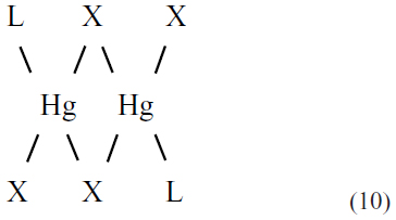
Table 2 lists the stability constants for some coordination complexes of mercury(I) and mercury(II) cations.15–17,19 Both ions bind relatively strongly to pyrophosphate (LogK =15.6, 17.5). For comparison, the stability constant for the complexation of mercury(II) with the common hexadentate ligand ethylenediaminetetraacetic acid is 21.5.19 Mercury(I) forms the most stable complexes with the dicarboxylates, such as oxalate (LogK =13) and succinate (LogK =13.5), while mercury(II) binds more strongly to the monocarboxylates acetate (LogK =23.2) and formate (LogK =9.6). Both mercury(I) and mercury(II) form relatively stable complexes with aniline (LogK =3.7, 4.6); however, only mercury(II) binds strongly to the amino acids due to their higher basicity (pKa >8.8). Mercury(II) also binds very strongly to ligands containing an SH group, including the amino acid cysteine (LogK =14.4).
| Table 1 Stability constants for complexes formed by mercury(I) and mercury(II) in aqueous solution at 25°C |
Mercury(II) is known to bind strongly to natural humic materials found throughout aqueous environments. These natural dissolved organics are also strong chelating agents with other trace metals in natural waters.20 They are thought to be derived from the decomposition of plant materials and thus vary in composition depending on their source and location. These humic compounds have a wide range of molecular weights, from a few hundred to several hundred thousand Daltons. The major binding sites in these natural humic materials are oxygen, primarily carboxylic acids (30%–50%), nitrogen (1%–4%), and reduced sulfur (1%–2%).21 Due to the prevalence of carboxylic acid groups, the higher molecular weight fractions are known as humic acids, while those in the smaller molecular weight range are fulvic acids. Most aqueous trace metals are generally bound to the more available oxygen containing carboxylic acid sites. However, mercury(II) is expected to preferentially bind to the sulfur binding sites, which are present only in trace quantities.19 Binding to the carboxylic acid groups is thought to occur only after the sulfur binding sites have been saturated.
The stability constants of mercury(II) with humic materials are difficult to determine due to the variation in the chemical composition of the organics, the presence of competing complexing agents, and the extent of dissociation of the acid groups. The reported logK for the mercury(II) binding with aqueous humic materials varies from 10 to 28, with higher values attributed to sulfur binding and lower values to carboxylate complexation.19 It has been estimated that approximately 50%–90% of the total mercury in freshwater and coastal seawaters is complexed by humic and fulvic acids.22 Because humic acids contain few of the strongly binding reduced sulfur sites, it is likely that in natural aqueous systems, the complexation of mercury(II) by humics takes place at both reduced sulfur and carboxylic acid sites in a multidentate Hg-humic complex.
Mercury(II) can also form organometallic compounds of the form RHgX, R2Hg, and RHgR’ where R and R’ are organic radicals and X = Cl−, Br−, I−, OH−, SO42−, CO32−, PO42−, and NO32−. The properties of the RHgX organomercury(II) compounds depend strongly on the nature of X and the Hg-X bond.15 If X is an anion with a large, highly polarizable electron shell, such as Cl−, Br−, I−, or OH−, the Hg-X bond will be covalent and nonpolar, and the organomercury compound will be lipophilic. If X is an anion with a poorly deformed electron shell, such as SO42−, CO32−, PO42−, or NO32−, the Hg-X bond will be ionic and the organomercury(II) compound will be hydrophilic. The most common environmental forms of organic mercury(II) compounds are methylmercury(II) (CH3Hg’) and dimethylmercury(II) (CH3Hg CH3). Due to the low polarity of the C-Hg bond, methylmercury(II) and dimethylmercury(II) are not readily decomposed by oxygen in air or water. However, they can be decomposed by exposure to light or heat. Dimethylmercury is volatile, with a Henry’s law constant similar to elemental mercury (see Table 1).
Cobalt-containing organic compounds with Co-CH3 bonds such as methyl cobalamin, an active form of vitamin B12, can react with mercury(II) to form CH3-Hg’, transferring the methyl group from cobalt to mercury as shown in Figure 4.23 There are a number of microorganisms in aqueous systems that can perform this same function, biochemically methylating mercury(II) and transforming it into the methylmercury(II) cation and subsequently dimethylmercury(II). The biochemical mechanism is thought to be similar to that with methyl cobalamin. It has also been shown that mercury(II) can be effectively methylated by an abiotic mechanism involving natural humic acids.22 The methylation of mercury(II) is dependent on the amount of free mercury available. Therefore, strong complexation with dissolved sulfide or humic materials in the aqueous or sediment phase will attenuate mercury methylation rates.24
 | Figure 4 Methylation of mercury by methylcobalamine, a form of vitamin B12, to form the methylmercuric cation. |
In aqueous systems, the CH3Hg’ ion is hydrated, giving the pH-dependent reactions:
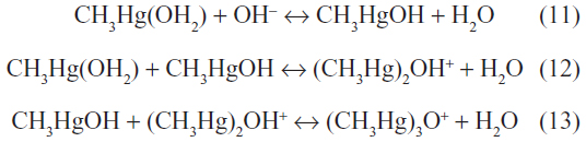
However, in the presence of high concentrations of Cl−, it readily combines to yield the nonpolar lipophilic compound methylmercury chloride (CH3HgCl). The CH3Hg’ ion also binds strongly to sulfur-containing and selenium-containing proteins and peptides, forming monomeric nonpolar complexes of the form CH3HgSR.9 This is in contrast with the Hg2+ cation, which binds to sulfur-containing proteins to form polymeric polar complexes. The CH3Hg’ ion can also bind to natural humic and fulvic acids. Binding studies have determined two classes of binding sites with conditional stability constants (logK) of 13–14.5 and 12–13.24 Equilibrium distribution calculations show that most of the dimethylmercury(II) ions in oxidized fresh waters are in the form of humic complexes. In anoxic waters with higher sulfide content, the CH3HgSH would predominate.25
Toxicity and bioaccumulation of mercury
Although all forms of mercury are toxic, they differ in their degree of toxicity and in their biological effects. Exposure to elemental mercury occurs primarily through inhalation of the mercury vapor. Atmospheric concentrations are sufficiently low that acute toxicity exposures happen only when there is a mercury spill or at highly contaminated sites. However, increased levels in the atmosphere may have long-term chronic effects. Approximately 80% of inhaled elemental mercury is absorbed, in contrast with less than 1% absorption after dermal exposure, and almost none (0.1%) after ingestion.26,27 Mercury vapor is a highly diffusible, monatomic gas. It is soluble in lipids, with a heptane/water partition coefficient of 20.28 The primary site of absorption of elemental mercury into the bloodstream is through the alveoli. Once in the bloodstream it is rapidly oxidized to mercury(II) in the red blood cells by way of the hydrogen peroxide catalase pathway.27 This is consistent with the observations that the distribution of elemental mercury in tissues is similar to that observed for mercury(II) salts. The half-life of elemental mercury in the body is reported to be approximately 60 days.27
Although mercury(I) chloride was used medicinally as a diuretic in the 1800s, very few studies have been reported on the biological effects of mercury(I) compounds. Due to its very low water solubility, mercury(I) chloride was assumed to be poorly absorbed in the gastrointestinal tract. However, high tissue levels of mercury(II) have been reported after ingestion of mercury(I) chloride. The mercury(I) that is absorbed after ingestion is therefore thought to be rapidly converted to mercury(II).28 The toxicity and biological effects for both mercury(I) and mercury(II) compounds have thus been reported together under the generic term “inorganic mercury”. Exposure to inorganic mercury can occur both through ingestion of inorganic mercury salts or inhalation of the aerosols, with absorption rates of about 10% for both ingested and inhaled inorganic mercury compounds.29 Inorganic mercury compounds have low lipid solubilities and therefore do not easily cross biological membranes. However, once absorbed, the ability of mercury(II) to bind strongly to cysteine residues in proteins acts to enhance the lipid solubility and aid in membrane transport. Mercury(II) is also highly reactive to enzymes containing sulfur or selenium, irreversibly inactivating them. In addition, mercury(II) can be converted to methylmercury by microorganisms in the intestinal tract.30 The half-life of inorganic mercury compounds in the body is reported to be approximately 40 days.27
The most common organometallic mercury(II) compound in environmental systems is methylmercury. Although inhaled methylmercury is absorbed as efficiently as elemental mercury (80%), the major source of human exposure to methylmercury is ingestion of contaminated fish.26 Methylmercury produced biochemically by microorganisms is taken up by aquatic plants and animals and is biomagnified through the aquatic food chain, with the highest concentrations found in the top predators. The US Environmental Protection Agency has issued approximate bioaccumulation factors (BAF) for methylmercury in aquatic systems. In general, the BAF for microorganisms in trophic level 2, such as zooplankton, are 1×10⁵; the BAF for the primary carnivores in trophic level 3 are 7×10⁵; and the BAF for the secondary carnivores in trophic level 4, including fish and birds, are 3×106.31 Therefore, levels of methylmercury in large fish are, on average, a million times the concentration of methylmercury in the water. However, the BAF suggested by the Environmental Protection Agency are based on an average of different species of fish living in different types of water bodies. The BAF for lake fish is three times higher than that for river fish. In addition, the body burden of methylmercury varies widely by fish species, age, and location, as well as type of water body.
Since methylmercury is highly lipid-soluble and will bind to cysteine residues, it is readily transported across membranes. About 95% of ingested methylmercury is absorbed in the gastrointestinal tract regardless of the speciation or method of ingestion, and a stable tissue distribution is reached within about 3 days.28 Methylmercury readily reacts with sulfhydryl groups interfering with cellular structure, enzyme function, and protein synthesis. It is slowly broken down to mercury(II) by demethylation, presumably by microflora in the intestines, which leads to increased elimination. The half-life of methylmercury in the body is reported to be 70–80 days.28
Atmospheric mercury trends
Since mercury is naturally occurring and found throughout the world, there are many natural emission sources that result in a background level of mercury in the environment. This low level mercury background level has existed since before recorded history. However, historical records obtained from measurements made in ice cores, lake sediments, and peat show that environmental mercury levels have increased considerably since the beginning of the industrial age.32 Measurements of long-term atmospheric mercury deposition to the Upper Fremont Glacier in Wyoming shown in Figure 5 are a good indication of the historical trend of mercury in the atmosphere over a period of 270 years.32,33 Measurements at this high altitude, remote location suggested a preindustrial background concentration of 3–4 ng/L when not influenced by short-term emissions (<2 years) from volcanic activity, such as the Mount Tambora eruption in Sumbawa, Indonesia, in 1815 AD. Significant increases over this background level in Upper Fremont Glacier samples generally coincide with changes in human activities from 1848 to the present day.
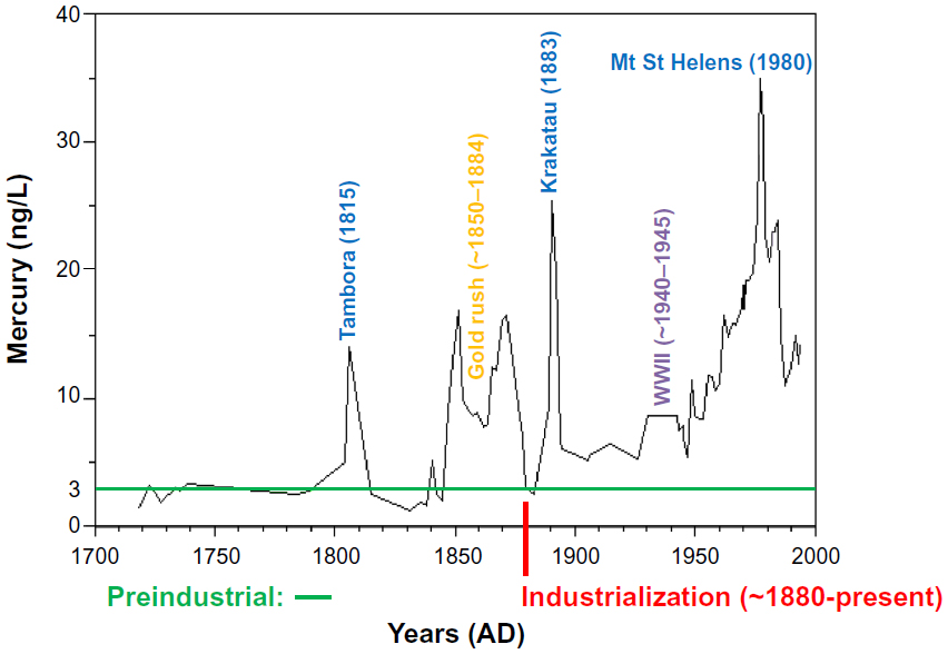 | Figure 5 Mercury concentrations measured in ice cores obtained from the Upper Fremont Glacier in the Wind River Mountain Range of Wyoming. |
Atmospheric mercury deposition was observed to increase from 1848 to around 1885, coinciding with the increased use of mercury in hydraulic gold mining operations throughout the western USA during this period. These mining operations were the most significant anthropogenic source of mercury in the first 170 years covered by the Upper Fremont Glacier record and peaked around 1860 and again about 1877.32 The use of mercury in gold mining ended in 1884 with the Sawyer decision, which banned the use of hydraulic mining due to the pollution and environmental damage it caused. This end to hydraulic mining was accompanied by a decrease in mercury concentrations in the Upper Fremont Glacier samples to approximately background levels. The mercury signal from the eruption of the Krakatoa super caldera occurred in 1883, shortly after the decline from the gold rush era. The increased mercury emissions from Krakatoa dissipated around 1885, returning to a steady level of about 6–7 ng/L. Mercury deposition increased again to levels of about 10 ng/L from about 1930 to 1945, corresponding roughly to the increased mobilization during World War II. After 1945, mercury levels continued to rise, with a peak in the 1980s that was 20 times higher than preindustrial levels.
Results from the Upper Fremont Glacier samples indicate that during the last 100 years there has been a 70% rise in atmospheric mercury levels over the natural background levels measured prior to industrialization. This trend is similar to that obtained from lake sediment measurements made in the upper Midwest.34 However, recent mercury concentrations in the Upper Fremont Glacier samples were seen to decline during the 1990s, from the peak value of 20 times the background levels to approximately eleven times the preindustrial levels.32 This recent downward trend is consistent with direct measurements of atmospheric mercury made worldwide.35
Sources of mercury emission to the atmosphere
In February 2005, the Governing Council of the United Nations Environment Programme issued a mandate that:
“Requests the Executive Director to facilitate work between the mercury programme of the United Nations Environment Programme and Governments, other international organizations, non-governmental organizations, the private sector and the partnerships, as appropriate: a) To improve global understanding of international mercury emission sources, fate and transport; b) To promote the development of inventories of mercury uses and releases; c) To promote the development of environmentally sound disposal and remediation practices; d) To increase awareness of environmentally sound recycling practices”.36
In keeping with this mandate, there have recently been a number of intensive studies aimed at improving our knowledge of mercury emissions to the atmosphere on a global scale. The most recent studies have provided revised global assessments of mercury emission sources as well as new scenarios of projected future mercury emissions.37–40
In assessing the importance of mercury emissions to the atmosphere, it is important to distinguish between the different types of sources. The sources of mercury emissions can be grouped into three major categories:41 natural sources or releases due to the natural mobilization of geological mercury from the earth’s crust; current anthropogenic sources including both release of mercury from raw materials as well as release of mercury used intentionally in products and processes; and historic anthropogenic sources that result from remobilization of mercury previously deposited from the atmosphere to soil, water, and vegetation. The global mercury assessment issued by the United Nations Environment Programme in 2013 estimated that 5,500 to 8,900 tonnes (1 tonne =1 Mg) of mercury are emitted directly to the atmosphere each year, and of this, approximately 10% is from natural sources, 30% is from current anthropological sources, and 60% is from re-emission of historical anthropogenic mercury deposits.41
Natural sources
Natural sources of mercury emissions to the atmosphere are those that arise from totally natural processes without any anthropogenic intervention. These sources are responsible for the background atmospheric mercury levels shown in Figure 5 prior to 1845. Natural sources of mercury include geothermal activities, volcanic eruptions, natural volatilization from the ocean surfaces, and weathering of mercury-containing minerals. Natural emissions of mercury to the atmosphere are low compared with the total global mercury emissions with an estimated total amount of 643 tonnes annually.38,39
One potentially important natural source of mercury is from geothermal activities and volcanic eruptions. Geothermal fluids are known to be enriched in trace metals, such as gold, silver, arsenic, antimony, and mercury, from the high temperature dissolution of the substrate minerals over time. The dissolution and transport of mercury in geothermal fluids is determined by temperature, pH, redox state, and concentrations of typical complexing agents in the fluids, as well as the types of subsurface minerals present in the system. When reducing geothermal fluids (where HS− is dominant over SO42−) are in the presence of cinnabar, geochemical calculations show that elemental mercury is abundant at temperatures above 200°C.42 Increasing temperature and pH along with decreasing ionic strength, pO2, and total sulfur all favor formation of elemental mercury. As these geothermal fluids mix with oxidizing or acidic water, formation of mercury(II) is favored, resulting in reprecipitation of cinnabar. Thus, emissions of mercury from these systems are caused by thermal release of mercury from the hot mercury-enriched substrate in contact with the reducing geothermal fluid followed by volatilization of elemental mercury to the atmosphere driven by heat flow.43 Mercury emissions from quiescently degassing geothermal systems, such as hot springs and fumaroles, exhibit spatial and temporal variability that depend on the age and type of geothermal system. The current estimate for the global emission of mercury to the atmosphere from geothermal activity is 60 tonnes annually, which is 9% of the total atmospheric emissions from natural sources (see Figure 6).44 Although the amount of mercury emitted to the atmosphere from geothermal activities is not large on a global scale, it may be of environmental concern on a local or regional scale if geothermal energy is to be actively pursued as an alternate energy source.
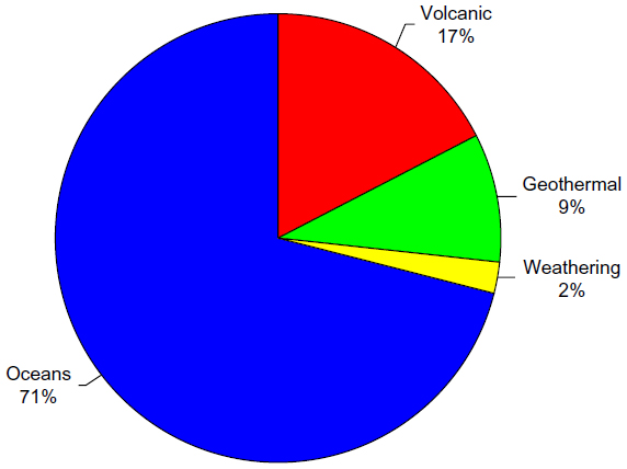 | Figure 6 Relative contributions of estimated mercury emissions to the atmosphere from natural sources. |
Mercury is released from active volcanoes by much the same mechanism as in geothermal systems. Elemental mercury is volatilized from the hot lava under reducing conditions and is emitted to the atmosphere along with other hot gases. The contribution of mercury emissions from volcanoes also varies over time and space depending on the number, location, and eruptive phase of the active volcanoes. As seen in Figure 5, a major eruption can result in atmospheric mercury levels that are 4–6 times those prior to the eruption, and the atmospheric burden from a single large volcanic eruption lasts approximately 2 years. There are currently about 50–70 terrestrial volcanoes that are active to some extent. The amount of mercury released to the atmosphere from these eruptions varies according to the size, duration, and phase of the eruption and the subsurface geology of the volcano. The current estimate of total global mercury emissions from volcanic activity varies widely, ranging from one to about 700 tonnes per year.43 This wide range of estimates is due in part to the large variation in types and locations of the eruptions studied. The release of mercury from continuously erupting and degassing volcanoes is about 75 tonnes per year, whereas the release of mercury from smaller sporadic eruptions is <10 to 100 tonnes per event.43 Large explosive eruptions account for only 15% of total volcanic mercury emissions. However, the occurrence of several large eruptions per century could result in the release of >1,000 tonnes of mercury to the atmosphere, overwhelming the total atmospheric burden over short periods of time. The total global flux of mercury to the atmosphere from volcanic activity is estimated to be about 112 tonnes per year, accounting for 17% of the total atmospheric emissions of mercury from natural sources (see Figure 6), with large variations in regional emissions.45
The direct low temperature emissions from the weathering of mineralized mercury deposits to aquatic and terrestrial environments could conceivably occur through sediment transport and wind-blown dusts. However, the most abundant form of naturally occurring mineralized mercury, cinnabar, is highly resistant to low temperature oxidation and weathering processes and is insoluble in water. The low temperature emission of mercury from mineral deposits directly to the atmosphere can occur by volatilization if a significant portion of the mercury contained in the mineral is in elemental form. The rate of volatilization would then depend on the amount of elemental mercury in the mineral deposit and meteorological parameters, such as temperature and wind speed. Although elemental mercury has been found in highly enriched mercury mineral deposits, such as in the New Idria mercury mine in California, these areas have also been subject to mining activities, and the mercury emissions are largely attributed to these anthropogenic operations. There is little evidence that elemental mercury exists naturally in environmentally relevant amounts in minerals or soils found outside these localized enriched mineral deposits. It has been estimated that the natural emissions of mercury to the atmosphere from mineralized areas are in the order of 10–20 tonnes per year, approximately 2% of the total atmospheric mercury emissions from natural sources.41 However, it is still unclear how much of these releases are due to purely natural processes.
Perhaps the largest source of natural mercury emissions to the atmosphere is the release of volatile mercury species from ocean surface waters. Natural sources of mercury to the oceans include submarine hydrothermal vents and volcanic activity on the ocean floor and deposition of natural mercury emitted directly to the atmosphere.46 Hydrothermal vents form in volcanically active areas, often on mid-ocean ridges, where there are gaps in the tectonic plates. Hydrothermal fluids in these vents can reach temperatures as high as 400°C under the high pressures of the ocean floor. As in terrestrial geothermal systems, high temperatures and reducing conditions can leach elemental mercury from the mercury-enriched substrate. Concentrations of mercury in hydrothermal fluids are found to be 1,000 times higher than that in ambient seawater.47 As these geothermal fluids mix with cold, oxidized seawater, Hg2+ is formed, resulting in precipitation of cinnabar back to the sea floor, enhancing mercury concentrations in the vicinity of the hydrothermal vents. This settling of particulate matter to the sea floor may result in eventual burial to deep sea sediments, returning the mercury to the mineral reservoir, and acting as a long-term sink for environmental mercury. Recent estimates of present day burial of mercury-containing sediments are in the range of 180–260 tonnes per year.48 This particulate mercury(II) can also be re-reduced to elemental mercury, releasing it back into the water column. It has been shown that the thermophilic bacteria surrounding these hydrothermal vents are capable of reducing Hg2+ to elemental mercury, thus detoxifying the local environment while releasing the volatile elemental mercury into the open ocean where it can be carried to surface waters.47 The total amount of naturally derived mercury released from the surface ocean to the atmosphere is estimated to be 456 tonnes per year.38,48 This accounts for 71% of the atmospheric emissions of mercury from natural sources.
Current anthropogenic sources
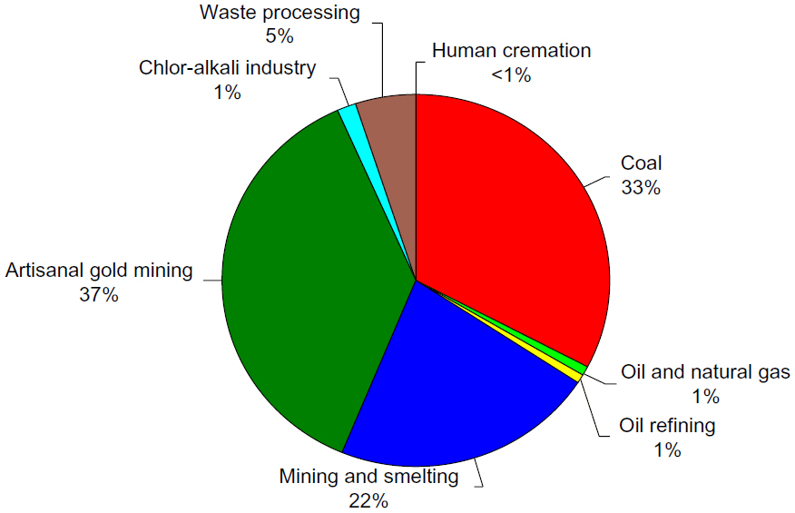
The relative contributions of major current anthropogenic sources to atmospheric mercury emissions, according to the 2013 United Nations Environment Programme global mercury assessment, are shown in Figure 7.44 The current anthropogenic sources of mercury emission to the environment fall into two major categories. The first is in processes where release of mercury occurs because it is present in fuels or raw materials as an impurity. Mercury emissions resulting from these impurities are sometimes referred to as “unintentional” or “byproduct” emissions. The main sources of atmospheric mercury in this category are coal burning (33%) and mining and smelting activities (22%), with minor contributions from combustion of oil and natural gas (1%) and oil refining (1%). The second category includes releases from products or processes where mercury is used intentionally. The largest source of atmospheric mercury in this category is small-scale gold mining (37%), followed by disposal or processing of waste from consumer products (5%). Other intentional sources of mercury emissions arise from its use in the chlor-alkali industry (1%) and release from dental fillings during human cremation (<1%).
 | Figure 7 Relative contributions of estimated mercury emissions to the atmosphere from current anthropogenic sources. |
The combustion of coal is the most significant source of “unintentional” current anthropogenic mercury emissions, resulting in the release of about 647 tonnes to the atmosphere each year, 33% of the total current anthropogenic emissions.44 Coal is used to fire kilns in cement production and in commercial and residential heating. However, more than 85% of mercury emissions from coal are from electrical power generation. The concentration of mercury in coal is relatively low, ranging from 0.01 to 1.5 g/Mg, with a worldwide average of about 0.1 g/Mg.38,49 However, the very large volumes of coal burned worldwide (6,118 Tg in 2006) result in large significant emissions from this source.38
The mercury that is emitted from electrical power plants is released directly into the atmosphere in any combination of three forms, ie, vapor phase elemental mercury, vapor phase mercury(II) compounds, or mercury that is adsorbed onto particulate surfaces.50 The major emission species are dependent on the type and moisture content of the coal and its combustion temperature. In general, the majority of mercury emission from combustion of bituminous coal is mercury(II), while the majority of mercury released from the combustion of sub-bituminous and lignite coal is elemental mercury.50 The amount of mercury released is also determined by the type and efficiency of emission control equipment used. Electrostatic precipitators and fabric filters are commonly used for particulate control worldwide, and while these technologies, if properly maintained, are efficient in removing >99% of the particulates produced in combustion, approximately 900 tonnes of particulates are still emitted to the atmosphere each year due to the large amounts of coal burned.51 Flue gas desulfurization units used to remove gas phase emissions, such as sulfur dioxide, are designed specifically to remove acidic species from combustion gases and thus are not very effective for controlling elemental mercury emissions.37–39,41 The major species emitted to the atmosphere from the combustion of coal in electrical power plants are the vapor phase species, ie, elemental mercury from lignite and sub-bituminous coal and mercury(II) from bituminous coal.
Mercury emission to the atmosphere from the combustion of oil and natural gas, which is estimated to be about 10 tonnes per year, is a minor contribution (1%) of the total current anthropogenic emissions compared with emissions from coal combustion.44 Fuel oils are used by some electrical power utilities and for commercial, industrial, and residential heating. The mercury content of fuel oils ranges from 0.01 to 30 g/Mg, with an average of 3.5 g/Mg.38 The heavier distillate fractions of fuel oils commonly used in residential heating contain higher levels of mercury while lighter distillate fractions contain less mercury. The mercury content of natural gas varies widely from 0.01 to 5,000 μg/m3 depending on the geological location.52 However, since mercury can amalgamate with other metals commonly used in gas processing plants, causing corrosion of equipment, efforts are usually made to remove mercury from the gas stream before processing. The magnitude of mercury emissions from natural gas combustion depends on the mercury content of the gas before processing and the extent to which mercury removal has been achieved.
Oil refining is estimated to release approximately 16 tonnes per year of mercury to the atmosphere, representing 1% of total current anthropogenic emissions.44 As with natural gas, mercury levels in crude oil can be widely variable, both between and within reservoirs. Releases of mercury to the atmosphere during the refining process are low because petroleum refineries also make an effort to remove mercury from the crude before processing due to problems associated with amalgamation of aluminum in refining equipment. However, common methods of mercury removal use disposable solid adsorbents. These mercury-containing adsorbents are released in industrial solid waste, which is disposed of in landfills. The mercury contained in this industrial waste may slowly be leached into aquatic and terrestrial environments. An estimated 0.6 tonnes per year of mercury is released to aqueous environments from oil refining.44
Mining and industrial processing of ores are important global sources of mercury emissions to both air and water. Mining and ore processing involve extraction of the desired metals from the surrounding minerals. The ore is processed by crushing and washing, followed by various physical or chemical separation processes. Often, the ore goes through a refining process that includes chemical reduction followed by heating the ore to high temperatures. This process releases elemental mercury into the air while other metals remain behind. The amount of mercury released in this process depends on the concentration of mercury in the ore.
Estimated total global emissions from mining and ore processing are approximately 430 tonnes per year (22% of the total current anthropogenic emissions) to the atmosphere and 114 tonnes per year to aqueous systems.44 The releases directly to the atmosphere include: emissions from large-scale gold mining operations (97 tonnes per year); primary production of nonferrous metals, ie, aluminum, copper, lead, and zinc (193 tonnes per year); primary production of ferrous metals, ie, pig iron, cast iron, and steel (46 tonnes per year); and mercury mining operations (12 tonnes per year). The mining and extraction of mercury itself is currently a minor source of atmospheric emissions due to the preference for recycling and reuse as a source of mercury. However, mercury emission to soil and water from contamination sites associated with past mercury mining is estimated to be approximately 16.7 tonnes per year. Mercury emissions directly to the atmosphere from all contaminated mining sites, including abandoned mercury mines, are estimated to be approximately 83 tonnes per year.44
The major source of emissions to the atmosphere from the intentional use of mercury is from small-scale or artisan gold mining. In these small-scale processes, miners mix elemental mercury with finely crushed gold ore silt, which creates an amalgam, with the gold separating it from the minerals. The mercury is then removed from the amalgam by heating over an open flame, volatilizing the mercury directly to the atmosphere and leaving the gold behind. It is estimated that 95% of the mercury used in these artisan gold mining operations is released to the environment, with total mercury emissions of over 1,000 tonnes per year, representing 37% of all current anthropogenic emissions.38 Approximately 73% (727 tonnes per year) of emissions are released directly to the atmosphere from amalgam burning and volatilization from mine tailings.44 This practice is broadly dispersed worldwide, active in 70 countries, with at least a quarter of the world’s gold supply coming from these sources.37,38 Artisan gold mining is one of the most significant sources of mercury release into the environment in the developing world and is one of the most critical international environmental issues related to mercury emissions.
A major industrial use of mercury is the chlor-alkali industry. The chlor-alkali process uses mercury cell technology for electrolysis of sodium chloride solution to produce chlorine and caustic soda (sodium hydroxide). The cathode in the electrolytic cell is a thin layer of mercury. The saturated sodium chloride solution floats on top of the cathode. Chlorine is produced at the anode, and sodium is produced at the cathode, where it forms an amalgam with the mercury. The amalgam is continuously drawn out of the cell and reacted with water, which decomposes the amalgam into sodium hydroxide and mercury. The mercury is recycled back into the electrolytic cell. Mercury cells are becoming less common in the chlor-alkali industry as other more cost-effective and less toxic methods are becoming available. Currently, the use of mercury cells in the chlor-alkali industry results in the release of an estimated 28.4 tonnes per year of mercury to the atmosphere (1% of total current anthropogenic emissions) and 2.8 tonnes per year to aquatic systems.44
The emissions of mercury from waste disposal, processing, and recycling are related directly to the consumption of consumer goods. Although many products and processes that make use of mercury have been phased out due to toxicity, mercury is still used in a wide variety of products. These include batteries, electrical switches, fluorescent lamps, electronic devices, paints, pesticides and fumigants, medicines, cosmetics, and a wide range of measuring and control devices. After these products have outlived their usefulness, they are either deposited in landfills, incinerated, or recycled. While mercury in landfills may be slowly released into soil and water, incinerated waste can be a major source of mercury emissions to the atmosphere if insufficient emission controls are present. Worldwide emissions of mercury from consumer product waste disposal and processing is estimated at 95.6 tonnes per year to the atmosphere (5% of the total current anthropogenic emissions) and 89.4 tonnes per year to aquatic systems.44
A minor intentional emission source of mercury is from its use in dental amalgams. An estimated 3.6 tonnes per year of mercury, less than 1% of the total current anthropogenic emissions, are emitted to the atmosphere from dental fillings when bodies are cremated.44 Also, mercury can be released during production of the amalgam and preparation of fillings, and from disposal of removed fillings. Approximately 340 tonnes of mercury are used in dentistry per year, of which about 20%–30% is disposed of as solid waste.38 Dental use of mercury is declining, particularly in higher income countries, but the rate of decline varies widely. Use of dental amalgams is still significant in some countries, while in others the practice has all but ceased. In many lower income countries, increasing access to dental care may actually increase mercury use temporarily.
The regional distribution of current anthropogenic mercury emissions to the atmosphere is presented in Table 3.44 The largest amount of current anthropogenic atmospheric mercury emissions is from Asia, with a total of 931 tonnes per year, representing 47.6% of total global mercury emissions. Approximately 75% of Asian emissions come from the People’s Republic of China.44 The primary source of mercury emissions throughout Asia is coal combustion. China is the largest coal producer and consumer in the world, using coal in coal-fired power plants, industrial boilers, and residential heating.38 Approximately 47% of mercury emissions from the People’s Republic of China and 81% of emissions from India are due to combustion of coal.53 The People’s Republic of China also has an additional large component from artisan gold mining. In Europe, approximately 52% of total mercury emissions to the atmosphere are from combustion of coal followed by consumer disposal and incineration of waste.44 Coal combustion and incineration of waste also account for most of the mercury emissions in the USA and North America. Mercury emissions from South America and Sub-Saharan Africa are largely due to artisan gold mining.
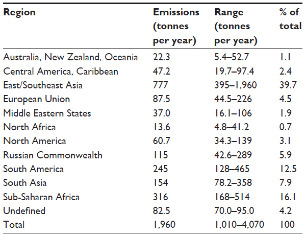 | Table 3 Distribution of current anthropogenic mercury emissions to the atmosphere by region |
A comparison of recent estimates with those reported from 1990 to 2005 shows that Europe and North America are reducing their mercury emissions. The USA has reduced emissions from coal-fired power plants by approximately 50% from 2005 to 2010.53 This relatively large reduction is primarily due to new regulations requiring both mercury and particulate controls on large power plants. However, emissions from Asia are increasing due to increased demands for energy. In addition, emissions from artisan gold mining have doubled since 2005, driven in part by increases in gold prices as well as increases in rural poverty in South America and Sub-Saharan Africa.
Historical anthropogenic sources
Mercury from historical anthropogenic emissions that has been previously deposited from the atmosphere to soil, water, and vegetation surfaces can be re-emitted back into the atmosphere. For this to occur, stable inorganic and organic mercury compounds in terrestrial and aqueous reservoirs must be converted into volatile mercury species, principally elemental mercury. After this occurs, re-emission is then generally dependent on temperature, with higher re-emission rates occurring at higher temperatures and lower re-emissions at lower temperatures. Once in the atmosphere, this volatile re-emitted mercury can then be transformed back into more stable oxidized species and redeposited onto surfaces, creating a cycling of mercury across the various environmental compartments, which is controlled by the oxidation-reduction chemistry of mercury. Due to the many variables involved in this process, re-emission rates are difficult to estimate and are often attempted through modeling approaches based on data for historical atmospheric mercury levels, deposition rates, and chemical transformation pathways.
The re-emission of previously deposited mercury should not be considered as a natural source of mercury emission to the atmosphere. Although mercury released from soil and water surfaces as well as from biomass burning may have a natural component, it is impossible to empirically determine the original source of these mercury emissions. The amount of mercury deposited to soil, water, and vegetation surfaces is a mixture of natural, recently deposited current anthropogenic, and cycled anthropogenic mercury. However, only 10% of mercury deposited from the atmosphere to surfaces is estimated to be of natural origin, and the levels of atmospheric mercury have increased by 70% since the beginning of the industrial era.48 Thus, 90% of the total mercury released by re-emission would be originally from anthropogenic sources and considered as an historical anthropogenic source.
One major pathway of mercury re-emission is through biomass burning. Mercury is deposited from the atmosphere onto plant surfaces by dry and wet deposition where it is assimilated into plant tissues by stomatal uptake. It accumulates in the leaves, needles, stems, and bark of plants and trees and has been shown to be an important net sink for atmospheric mercury under normal conditions.43 During biomass burning events, the re-emitted mercury released in smoke plumes includes that from both live and dead vegetation as well as from soil located beneath the vegetation. The mercury in smoke plumes has been shown to be 95% elemental mercury and 5% associated with particulates.54 Average global re-emission of mercury due to biomass burning from 1997 to 2006 has been estimated at approximately 675 tonnes per year, accounting for 14% of total historical anthropogenic emissions (see Figure 8).55
 | Figure 8 Relative contributions of estimated mercury emissions to the atmosphere from historical anthropogenic sources. |
The low temperature emission of mercury from soils and vegetation litter is significantly influenced by mercury speciation, meteorological conditions, and type of soil and litter. Mercury recently deposited from the atmosphere onto soil and ground litter is initially loosely adsorbed on the surface as elemental mercury or as mercury(II) compounds. Unless oxidized to mercury(II), elemental mercury is rapidly re-emitted from the soil surface. Recently deposited mercury(II) can undergo heterogeneous reduction reactions to elemental mercury followed by re-emission. Soluble mercury(II) can also be transported downward into the soil profile through pore waters. While mercury(II) can bind to negatively charged particles in clays and soil minerals, this bond is relatively weak and the mercury can easily be displaced to the aqueous phase, leading to reduction and re-emission as elemental mercury. However, mercury(II) also binds strongly to reduced sulfur and carboxylic sites in soil organic matter, with binding constants (logK) of 22–23.56 This strong binding protects mercury(II) from reduction and re-emission until the organic matter is decomposed. Therefore, the majority of the mercury re-emitted to the atmosphere is from the recently deposited surface fraction. This leads to an average lifetime of anthropogenic mercury in soils of approximately 80 years and a lower than expected re-emission rate.57 The overall re-emission of mercury from soils back into the atmosphere is estimated to be approximately 1,754 tonnes per year, representing 37% of total historical anthropogenic emissions.38
The major source of historical mercury emissions to the atmosphere is ocean basins. It is generally assumed that elemental mercury is the major mercury species emitted to the atmosphere from surface waters. However, dimethylmercury has a Henry’s law constant similar to that of elemental mercury (see Table 1) and has been observed in appreciable amounts over the Atlantic.58 Dimethylmercury has been shown to be rapidly reduced to elemental mercury in the atmosphere, with a lifetime of a few days.
The re-emission of mercury from surface waters is dependent upon the concentration gradient between mercury in the surface water to that in the air, and is also dependent upon solar irradiation, and the temperature at the air-water interface.38 In surface waters, mercury is present primarily as mercury(II) complexes with hydroxide, chloride (equations 6 and 7), and humic materials. It has been estimated that >95% of mercury(II) in lake, estuarine, and coastal waters is bound to humic and fulvic acids, while the majority of mercury(II) in the open ocean is complexed with chloride.59,60 Reduction of mercury(II) in aqueous environments can be achieved by photochemical, chemical, or microbial processes. Recent studies have shown that photochemical reduction is the principal mechanism in unpolluted surface waters.59 The efficiency of the photoreduction of mercury(II) depends on the amount of reducible mercury and the intensity and wavelength of the radiation. Although the mechanism of photochemical reduction is not well understood, the reaction is enhanced by the presence of humic materials and oxidized iron or magnesium.
Photoreduction of mercury(II) results in production of aqueous elemental mercury, which is re-emitted to the atmosphere at a rate dependent on surface temperature and meteorological conditions. Estimates of mercury re-emissions to the atmosphere from the oceans are at 2,226 tonnes per year, representing 47% of total historical anthropogenic emissions.38,48 While this estimate is 472 tonnes per year, (10% higher than the emissions estimate for soil and vegetation surfaces), the emissions on an area basis are higher for the terrestrial surfaces than for oceans by a factor of 2. Mercury emission rates from lake surfaces are generally higher than those observed over oceans. The total historical anthropogenic emission from lake surfaces is estimated to be 96 tonnes per year, accounting for 2% of total historical anthropogenic emissions. These emissions on an area basis are three times higher for lakes than for oceans.38
Atmospheric transport and transformations
Atmospheric mercury is classified operationally into three categories, ie, gas phase elemental mercury, gas phase mercury(II) compounds called reactive gaseous mercury, and mercury(II) compounds associated with atmospheric particulate matter known as total particulate mercury. Most of the mercury emitted or re-emitted into the atmosphere is gas phase elemental mercury (see Table 4) with minor amounts of gas phase mercury(II) compounds and particulate bound mercury(II).53,54 Elemental mercury is not significantly removed from the atmosphere by wet and dry deposition due to its relatively low deposition velocity and water solubility. It therefore remains in the atmosphere long enough to travel far from the source. However, oxidized mercury(II) compounds are removed more readily because of their higher water solubility and high reactivity with surfaces. It is thus estimated that over 95% of mercury in the atmosphere exists as elemental mercury.61 This atmospheric elemental mercury must first be oxidized to mercury(II) before being effectively removed from the atmosphere and deposited to soil, water, or vegetation surfaces.
| Table 4 Speciation of mercury emissions from different sources given as percent of total emissions |
The atmospheric oxidation of elemental mercury to mercury(II) is very important in the cycling of mercury from the atmosphere to other environmental compartments. It is also critical to estimation of the atmospheric lifetimes as well as atmospheric transport distances of mercury. The oxidation of elemental mercury to mercury(II) increases mercury deposition rates, while reduction of mercury(II) to elemental mercury increases its atmospheric lifetime. Therefore, understanding the oxidation-reduction chemistry of atmospheric mercury is critical in the understanding of mercury cycling through the environment. This chemistry, however, is still not well understood due to its complexity, as the oxidation of atmospheric elemental mercury can involve gas phase, aqueous phase, particulate phase, and heterogeneous reactions. Although there have recently been several reviews on the oxidation chemistry of mercury, most studies have concentrated on reaction kinetics, with few details on reaction mechanisms or product identification.53
The gas and aqueous phase reactions of mercury currently believed to be the most important in atmospheric removal processes have been summarized by several reviewers and are listed in Table 5, with their estimated rate constants and atmospheric mercury lifetimes calculated from the chemical kinetics for each reaction.53,61 It is important to note that the calculated lifetimes in Table 5 are chemical lifetimes based on the relative oxidation potentials of the various reaction pathways as determined in the laboratory and do not represent the actual lifetime of mercury in the atmosphere. Since atmospheric mercury is not irreversibly oxidized but undergoes an oxidation-reduction cycle, the actual lifetime of mercury in the atmosphere would be determined from the rates of competing oxidation and reduction reactions along with those of the physical removal processes.
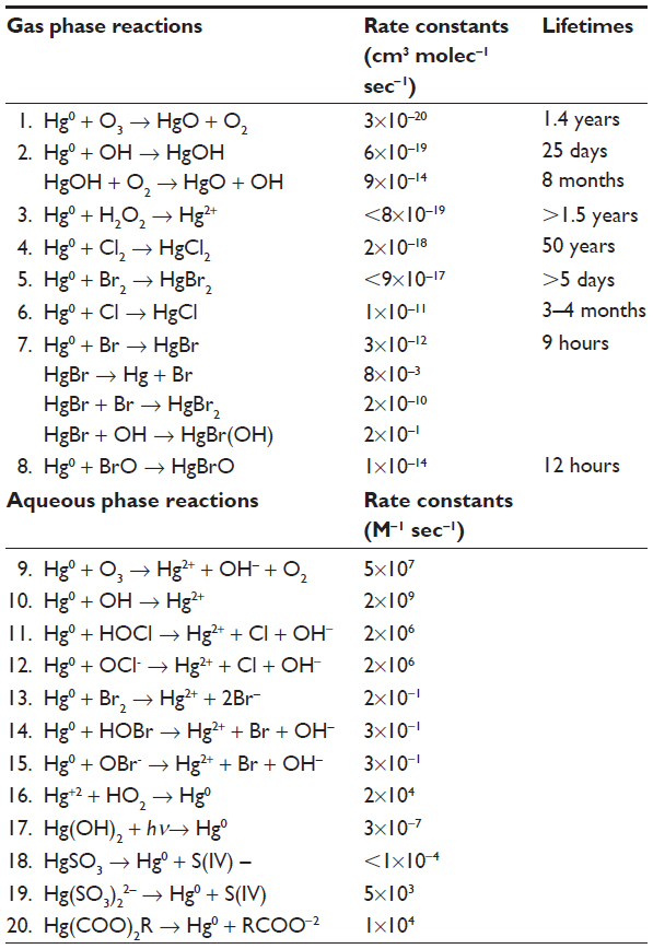 | Table 5 Important reactions of mercury relevant to the atmosphere with overall rate constants and atmospheric mercury lifetimes estimated from reaction kinetics |
The gas phase reactions are dominated by oxidation of elemental mercury to mercury(II) while both oxidation and reduction can occur in the aqueous phase. Originally, the major oxidation pathways for elemental mercury were thought to be the gas phase and aqueous phase reactions with ozone (Table 5, reactions 1 and 9). Early kinetic studies of the ozone mercury reaction resulted in a rate constant of 3×10⁻²⁰ cm3 molec−1 sec−1, which gave an estimated atmospheric lifetime for mercury of approximately 1.4 years.61 Atmospheric models using this early value for the rate coefficient were able to reproduce the observed atmospheric mercury concentrations. However, more recent studies have resulted in rate constants closer to 6×10⁻¹⁹ cm3 molec−1 sec−1, suggesting a lifetime of 20–30 days.53
The gas phase reaction of elemental mercury with ozone has been brought into question as there is now evidence suggesting that the primary reaction product is HgO3, which can then decompose to the observed products HgO and O2 on the walls of the reaction chamber.62 In the atmosphere, the decomposition of HgO3 is expected to occur on wet aerosol surfaces to form Hg(OH)2. This heterogeneous decomposition of the intermediate product HgO3 in the atmosphere complicates the reaction kinetics and may be responsible for atmospheric reaction rates that are very different from those observed in the laboratory. The reaction of elemental mercury with ozone in the aqueous phase was determined to be much faster than that in the gas phase. It was suggested that the mechanism likely involves an Hg-H2O2 complex, with the primary oxidation product being Hg(OH)2.58 Extrapolation to the concentrations and conditions typical of cloud water yielded a lifetime of approximately 5 days for mercury in cloud and an overall lifetime for atmospheric mercury of about 2 months.
The gas phase oxidation of elemental mercury by the OH radical to yield HgOH (Table 5, reaction 2) gave a reaction rate constant of 9×10⁻¹⁴ cm3 molec−1 sec−1 with an estimated atmospheric lifetime of approximately 8 months.63 However, recent mechanistic studies have determined that the reaction of elemental mercury with the OH radical is greatly attenuated by fast decomposition of the initial product, HgOH, back to Hg0 and OH. In addition, there are many other trace gases and aerosol surface species in the atmosphere competing for reaction with OH. Oxidation of elemental mercury by the OH reaction is therefore probably not an effective removal process.62
Oxidation of mercury by halogens was suggested as a possible explanation for mercury depletion events, where elemental mercury in the springtime atmosphere of the Arctic and Antarctic was seen to be rapidly converted to mercury(II). Although the reaction of elemental mercury with chlorine was determined to be too slow to be atmospherically important, the reactions with bromine atoms and BrO radicals were fast, leading to an estimated lifetime for atmospheric mercury of less than one day in areas where these species are present in sufficient concentrations.64 Atmospheric bromine atoms can be produced from sea spray during refreezing of open water areas between sea ice in the polar spring, and in the upper troposphere from photolysis of organobromides.53 The reactions of elemental mercury with bromine in these areas could significantly reduce the atmospheric lifetime of mercury. However, theoretical calculations of the oxidation reactions with bromine have determined them to be temperature-dependent, with faster reaction rates and shorter mercury lifetimes at the colder temperatures found at the poles and in the upper troposphere. This is because the initial product, HgBr, is stabilized at colder temperatures. While reactions at 245°C give an estimated atmospheric lifetime for mercury of 10 hours, reactions at temperatures above 280°C in the mid-latitude marine boundary layer increase the expected mercury lifetime to more than 4,000 hours (ie, about half a year).65–67
Studies of the distribution of mercury between the northern and southern hemispheres, as well as the temporal and spatial variability, imply a lifetime of about one year.58,67 In order to reconcile the mercury lifetimes based on atmospheric reaction kinetics with the observed spatial distribution of atmospheric mercury, either the gas phase kinetics in the atmosphere must be slower than those determined in the laboratory or the gas phase oxidation reactions must be balanced with reduction reactions that reform elemental mercury.66 There are no known atmospherically important reduction reactions in the gas phase. However, mercury(II) can be reduced in the aqueous phase (Table 5, reactions 16–20). One important suggested reduction reaction occurs via a two-step reduction by HO2/O2−.61
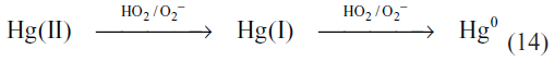
However, comparison of the one electron reduction potentials under ambient conditions showed that the two-step reduction should not occur due to the rapid reoxidation of mercury(I) by dissolved oxygen before the second electron transfer can take place.67
The remaining important reduction mechanism for mercury(II) in the aqueous phase is photoreduction in the presence of dicarboxylic acids (Table 5, reaction 20).68 The reaction rates for the photoreduction of mercury by oxalic, malonic, and succinic acids at pH 3 were reported to be 1×10⁴, 5×10³, and 3×10³. It was suggested that the mercury(II) was reduced either by organic radicals formed by photolysis of the mercury(II)-carboxylic acid (Hg(COO)2R) complexes or by an intermolecular two electron transfer during photolysis of the Hg(COO)2R complex. The presence of the chloride ion was found to significantly reduce the reduction rate. This was thought to be due to competition complexation of chloride ion with the organo mercury complexation, and demonstrated that the formation of an Hg(COO)2R complex was likely to important to the reduction.
After reduction, mercury(II) can be removed from the atmosphere by wet and dry deposition. Wet deposition occurs by uptake of the soluble species into cloud droplets followed by rain or other forms of precipitation. Dry deposition can occur through gravitational settling of particulate matter or by direct adsorption of gas phase species to surfaces. All mercury species present in the gas phase can be adsorbed onto atmospheric particulate matter or scavenged into cloud droplets. However, since gas-liquid partitioning according to Henry’s law (see Table 1) is higher for mercury(II) compounds than for elemental mercury, mercury(II) is the major mercury species in the aqueous phase and therefore the major species removed in wet deposition. Recent studies have shown that wet deposition dominates in areas with frequent precipitation, while dry deposition is the main removal process in more arid regions.53
Since deposited mercury can be re-emitted to the atmosphere and redeposited, it can be transported long distances by repeated cycles of re-emission, transport, and deposition, sometimes called the “grasshopper effect”. One result of this repeated cycling is that mercury can be transported towards the colder polar regions where re-emission is less rapid. Atmospheric gaseous elemental mercury has a lifetime of about 10 hours in the polar regions because the oxidation reactions with bromine are faster at low temperatures.65 Therefore, deposition of mercury in the polar regions is enhanced over normal deposition rates due to this enhanced bromine oxidation, resulting in ever-increasing mercury concentrations in the polar regions.
Conclusion and future research to resolve uncertainties
The chemical reactions, speciation, and transport of mercury in the atmosphere and other environmental compartments are very complex and not yet completely understood. Modeling of the atmospheric loadings and deposition rates of mercury species is still in need of major improvement. Often models require significant alteration of emission factors and/or oxidation-reduction reactions in order to reproduce the concentrations of mercury observed in the atmosphere or in wet and dry deposition samples. Considering that there are still large uncertainties in the chemical kinetics and product identification of the known gas and aqueous phase reactions of mercury as well as in as yet unstudied heterogeneous reactions, this unpredictable model performance is not surprising. In addition, there are also uncertainties involved in the currently available field data for mercury, which the models use for validation. It has been suggested that even in cases where model results succeed in accurately reproducing field measurements, the errors in the model may coincidently compensate each other to yield overall results that agree with observations.53,69 In other words, the models may give the right answer for the wrong reasons.53 In order to increase the reliable performance of mercury models, uncertainties in the model variables must be reduced as much as possible through both reliable in-depth field measurements and detailed laboratory studies of the important chemical reactions of mercury in the environment.
Most modeling efforts have typically assumed that the major uncertainty in reproducing observed atmospheric mercury loadings lies in global emission inventories. A chemical transport model simulation of global atmospheric mercury concentrations resulted in an estimated uncertainty in total global mercury emissions by an approximate factor of 2.70 This effort included both current and historical anthropogenic emissions as well as natural emissions of mercury. A state-of-the-art inventory of current anthropogenic mercury sources on a global scale has recently been presented by the United Nations Environment Programme Chemicals Branch.53 The emission source category that was identified as most poorly quantified was that of uncontrolled small-scale artisan gold mining, particularly in the People’s Republic of China. This was followed by emissions from sources never before considered in the inventories, ie, nonferrous metal production, vinyl chloride manufacturing, and production and use of dental amalgam. However, much larger uncertainties are likely associated with emissions from historical anthropogenic sources.
The re-emissions of mercury previously deposited to surface waters are controlled by aqueous oxidation-reduction chemistry in competition with binding to both inorganic and organic ligands. Given that aqueous humic and fulvic acids are well known to be strong binding agents for a wide range of metals,20 they may facilitate the transport of oxidized mercury in surface and ground waters. They may also be active in recycling mercury back to the atmosphere by promoting photoreduction. The importance of each of these reactions will vary with the composition and properties of aqueous systems. Emissions of mercury from soil surfaces are controlled by the same aqueous phase reactions in soil pore waters as well as adsorption to mineral and organic surfaces. These competitive reactions for mercury in the aqueous phase and heterogeneous reactions in soil and pore waters have been inadequately studied under environmentally relevant conditions. It is therefore not surprising that historic re-emissions from terrestrial and ocean surfaces are poorly constrained.
Major uncertainties in the atmospheric chemistry of mercury are also a significant factor in modeling efforts that need to be improved. Our current knowledge of mercury oxidation and reduction reactions is based on a limited number of laboratory and theoretical studies carried out under conditions not necessarily relevant to the atmosphere.41 The kinetics of basic mercury oxidation reactions need to be better determined as a function of temperature to lower the current uncertainties in the available kinetic data for most of the common oxidants, particularly ozone, bromine, and hydrogen peroxide. Also, reaction mechanisms and products need to be identified under atmospherically relevant conditions. Detailed laboratory studies coupled with field measurements will be required to identify the reaction mechanisms and mercury species important in the atmosphere. However, our current field measurement methods are not capable of achieving mercury speciation beyond operationally defined gas phase elemental mercury, reactive gaseous mercury, and total particulate mercury. Therefore, improved analytical techniques capable of determining specific mercury species at atmospherically relevant concentrations also need to be developed in order to validate laboratory results.
The importance of oxidation and reduction reactions in fog, cloud water, and wet aerosol surfaces also need to be better understood. In particular, the reaction of mercury with hydrogen peroxide in the aqueous phase should be studied under both light and dark conditions. This reaction is currently not included in the list of important aqueous phase reactions of mercury relevant to the atmosphere (Table 5), although it has been suggested as a possible mechanism for the observed oxidation of mercury by ozone in the aqueous phase.58 It is interesting to note that this reaction had previously been neglected in the early modeling of atmospheric sulfur dioxide removal processes and was later found to be the key reaction for the conversion of sulfur dioxide to sulfuric acid in acid rain.71
Direct oxidation of elemental mercury by hydrogen peroxide is being used in wet scrubbers for removal of mercury from industrial stack gases and is therefore clearly a rapid reaction, which is likely acid-catalyzed.72 It should be noted that hydrogen peroxide has a Henry’s law constant of 10−8 atm-m3/mol, while oxygen and ozone have Henry’s law constants of 1 and 0.1 atm-m3/mol, respectively. Thus, hydrogen peroxide is likely responsible for oxidation of the small amounts of mercury observed in water solubility and Henry’s law laboratory studies.8,73 While nitrogen purging will effectively remove oxygen and ozone from laboratory water, it will not remove hydrogen peroxide, and this would explain the necessity of adding a small amount of reducing agent (stannous chloride) to the aqueous phase in order to prevent oxidation of mercury and obtain reproducible results.73
The aqueous phase reduction reactions of mercury(II) also need to be better understood. While the photoreduction of dicarboxylic acid-mercury(II) complexes has been demonstrated to be an important method for recycling oxidized mercury to elemental mercury,68 the potential role of humic-like substances (HULIS) has not been examined. Significant amounts of HULIS have been found in cloud water, wet aerosols, and precipitation comprising as much as 50% of the water-soluble species.74 These HULIS are produced from both anthropogenic and biogenic sources, including biomass burning in the form of wildfires, agricultural and trash burning as well as the atmospheric oxidation reactions of isoprene, monoterpenes, and sesquiterpenes emitted naturally from vegetation. Like aqueous humic and fulvic acids, HULIS contain multiple carboxylic acids and alpha-hydroxy and beta-hydroxy acids that would be efficient complexing agents for mercury(II), and may thus promote photoreduction in a manner similar to the diacids. This as yet unstudied photoreduction mechanism could be an important recycling process for elemental mercury in the atmosphere, which would lead to longer atmospheric lifetimes.
Complexation of mercury(II) by HULIS may also facilitate atmospheric removal by wet deposition. Both HULIS and aqueous humic and fulvic acids are well known to be strong binding agents for a wide range of metals,20 so may also promote transport of oxidized mercury in surface and ground waters and be active in recycling by redox reactions with free and bound metal species in these aqueous environments.
The effects of climate change on mercury cycling will be complex and have the potential to increase the uncertainties in model predictions. Increasing temperatures will favor re-emission of volatile mercury species, principally elemental mercury, from terrestrial and aqueous systems. Changes in vegetation and land use will also change emissions from soil surfaces. Changing temperatures may also change the reaction rates, affecting mercury cycling in ways that are difficult to predict without temperature-dependent kinetics. Clinical temperature variance may also change which atmospheric reactions are more favored. Rapidly increasing temperatures in the polar regions leading to thawing of the Arctic tundra and sea ice could result in release of large reservoirs of mercury.53
Increasing temperatures will also result in increased emissions of terpenoids from vegetation, which will increase the levels of HULIS in cloud water. Increasing temperatures and longer growing seasons are predicted to increase the occurrence of wildfires, which will also increase HULIS emissions. These same wildfires produce significant amounts of formaldehyde and other aldehydes that can photoxidize to increase HO2 radical concentrations in regional air masses. The increased formation of HO2 would increase the formation of hydrogen peroxide from the reaction:

This reaction is strongly dependent on HO2 levels since the reaction kinetics are second order in HO2. It is also favored at the low nitric oxide concentrations typical of regional atmospheres. Thus, climate change may result in an increase in aqueous phase oxidation of elemental mercury by hydrogen peroxide as well as in the HULIS that can act to bind oxidized mercury. This may lead to enhanced photoreduction and/or wet deposition of these complexed forms of mercury. The strength of the complexation of HULIS with oxidized mercury will need to be determined as well as the photochemical reduction potentials in order to determine the overall effects of these changes on atmospheric mercury levels. Once evaluated, these potential mechanisms should be incorporated into the models to develop a better ability to predict and determine mercury lifetimes.
Ultimately, comparison of the model results with comprehensive field measurements and well focused process and mechanistic studies will be needed to adequately assess the effects of increased mercury levels under climate change. This will require focused laboratory studies to identify important reactions and products, improved models that incorporate the increasing complexity of atmospheric sources, transformations and sinks, and improved analytical instrumentation to quantify relevant mercury species in the atmosphere, and will serve to validate the models. Recently compiled survey data comparing measured gas phase elemental mercury in different geographic regions across the globe can currently be used for model validation.75 However, without detailed measurements of atmospheric mercury species beyond operationally defined gas phase elemental mercury designation, any disagreement between models and field measurements cannot be adequately assessed. These intercomparisons using novel instrumentation developed to examine specific mercury forms including more detailed information on complexes and their recycling times in the atmosphere and various deposition environments will be needed if we are to develop a better fundamental understanding of how increased levels of mercury will impact the environment and human health now and in the future.
Disclosure
The authors report no conflicts of interest in this work.
References
Mason R, Pirrone N, Hedgecock I, Suzuki N, Levin L. Conceptual overview. In: Pirrone N, Keating T, editors. Hemispheric Transport of Air Pollution 2010. Part B: Mercury. New York, NY, USA: United Nations Publication; 2010. | |
United States Environmental Protection Agency. Mercury study report to congress: Executive summary. United States Environmental Protection Agency Reports, 1997. Available from: http://www.epa.gov/ttn/oarpg/t3/reports/volume1.pdf. Accessed June 16, 2014. | |
Fahlman BD. Materials Chemistry. Dortrecht, The Netherlands: Springer; 2007. | |
Huber ML, Laesece A, Friend DG; National Institute of Standards and Technology. The vapor pressure of mercury. NIST Reports. 2008;NISTIR 6643:1–56. Available from: http://www.boulder.nist.gov/div838/SelectedPubs/NISTIR.6643.pdf. Accessed July 15, 2014. | |
Kaleri CJ. Implementation issues: mercury transport and fate, combustion risk assessments in Region 6. In: Cohen L, Eicher AR, Koenig R, Tripodes J, editors. Proceeding of the 2000 International Conference on Incineration and Thermal Treatment Technologies, May 14–18, 2000, Portland, OR, USA. Irvine, CA, USA: University of California; 2000. | |
Glew DN, Hames DA. Aqueous nonelectrolyte solutions. Part X. Mercury solubility in water. Can J Chem. 1971;49:3114–3118. | |
United States Environmental Protection Agency. Soil screening guidelines: Part 5 Chemical-specific parameters. 1996. Available from: http://www.epa.gov/reg3hscd/risk/human/rb-concentration_table/chemicals/SSG_nonrad_technical.pdf. Accessed June 17, 2014. | |
Clever HL, Johnson SA, Derrick ME. The solubility of mercury and some sparingly soluble mercury salts in water and aqueous electrolyte solutions. J Phys Chem Ref Data. 1985;14:631–680. | |
Cotton FA, Wilkinson G, Advanced Inorganic Chemistry: A Comprehensive Text. 4th ed. New York, NY, USA: John Wiley and Sons; 1980. | |
Vanderzee CE, Swanson JA. The enthalpy of precipitation of mercury(I) chloride and the thermodynamic properties of aqueous mercury(I) and mercury(II) ions. J Chem Thermodyn. 1974;6:827–843. | |
Dry ME, Gledhill JA. The solubilities of sparingly soluble salts in water. Part 4. The solubility of mercurous chloride at 25°C. Trans Faraday Soc. 1955;51:1119–1124. | |
National Research Council. Toxicological effects of methylmercury. National Research Council Reports. 2000. Available from: http://www.nap.edu/openbook.php?isbn=0309071402. Accessed June 17, 2014. | |
Iverfeldt A, Lindqvist O. The transfer of mercury at the air/water interface. In: Brutsaert W, Jirka GH, editors. Gas Transfer at Water Surfaces. Dortrecht, The Netherlands: Springer; 1984. | |
Sillman S, Marsik F, Al-Wali KI, Keeler GJ, Landis MS. Reactive mercury in the troposphere: model formation and results for Florida, the northeastern United States, and the Atlantic Ocean. J Geophys Res Atmos. 2007;112:D23305. | |
Chipperfield JR. Complexes of mercury(I) with oxygen-donor ligands. In: Zuckerman JJ, Hagan AP, Chipperfield JR, editors. Inorganic Reactions and Methods: Formation of Bonds to Group I, II, and IIIB Elements, Volume 13. Hoboken, NJ, USA: John Wiley and Sons; 2007. | |
Yamane T, Davidson N. Complexes of mercury (I) with pyrophosphate and dicarboxylate anions and mercury(II) pyrophosphate complexes. J Am Chem Soc. 1960;82:2123–2129. | |
Wirth TH, Davidson N. Studies of the chemistry of mercury in aqueous solution. I. Mercury(I) and mercury(II) complexes of aniline. J Am Chem Soc. 1964;86:4314–4318. | |
Kozin LF, Hansen S. Mercury Handbook: Chemistry, Applications and Environmental Impact. Cambridge, UK: Royal Society of Chemistry; 2013. | |
Ravichandran M. Interactions between mercury and dissolved organic matter – a review. Chemosphere. 2004;55:319–331. | |
Gaffney JS, Marley NA, Orlandini KA. The use of hollow fiber ultrafiltraters for the isolation of natural humic and fulvic acids. In: Gaffney JS, Marley NA, Clark SB, editors. Humic and Fulvic Acids: Isolation, Structure, and Environmental Role. Washington, DC, USA: American Chemical Society; 1996. | |
Gaffney JS, Marley NA, Clark SB. Humic and fulvic acids and organic colloidal materials in the environment. In: Gaffney JS, Marley NA, Clark SB, editors. Humic and Fulvic Acids: Isolation, Structure, and Environmental Role. Washington, DC, USA: American Chemical Society; 1996. | |
Weber JH. Review of possible paths for abiotic methylation of mercury(II) in the aquatic environment. Chemosphere. 1993;26:2063–2077. | |
Walker BC. Organic Pollutants: An Ecotoxicological Perspective. Boca Raton, FL, USA: CRC Press; 2009. | |
Hammerschmidt JH, Fitzgerald WF, Balcom PH, Visscher PT. Organic matter and sulfide inhibit methylmercury production in sediments of New York/New Jersey harbor. Marine Chem. 2008;109:165–182. | |
Hintelmann H, Welbourn PM, Evans RD. Measurment of complexation of methylmercury(II) compounds by freshwater humic substances using equilibrium dialysis. Environ Sci Technol. 1997;31:489–495. | |
Bernhoft RA. Mercury toxicity and treatment: a review of the literature. J Environ Public Health. 2012;2012:460508. | |
Broussard LA, Hammett-Stabler CA, Winecker RE, Ropero-Miller JD. The toxicology of mercury. Lab Med. 2002;33:614–625. | |
Clarkson T, Cranmer J, Sivulka D, Smith R. Mercury health effects update: health issue assessment. Environment Protection Agency Reports, 1984. Available from: http://cfpub.epa.gov/ncea/cfm/recordisplay.cfm?deid=33398. Accessed July 15, 2014. | |
Bull S. HPA compendium of chemical hazards: inorganic mercury/elemental mercury. Environment Protection Agency Reports, 2011. Available from: http://www.hpa.org.uk/webc/HPAwebFile/HPAweb_C/1194947406874. Accessed March 14, 2014. | |
Rowland IR, Robinson RD, Doherty RA. Effects of diet on mercury metabolism and excretion in mice given methylmercury: role of gut flora. Arch Environ Health. 1984;39:401–408. | |
United States Environmental Protection Agency. Water quality for the protection of human health: methylmercury. Environment Protection Agency Reports, 2001. Available from: http://water.epa.gov/scitech/swguidance/standards/criteria/health/upload/mercury2010.pdf. Accessed June 17, 2014. | |
Schuster PF, Krabbenhoft DP, Naftz DL, et al. Atmospheric mercury deposition during the last 270 years: a glacial ice core record of natural and anthropogenic sources. Environ Sci Technol. 2002;36:2303–2310. | |
Schuster PF, Krabbenhoft DP, Naftz DL, et al; NOAA/NGDC Paleoclimatology Program. Fremont Glacier atmospheric mercury data, IGPB. PAGES/World Data Center for Paleoclimatology Data Contribution Series 2002. Available from: http://www.ncdc.noaa.gov/paleo/pubs/schuster2002/schuster2002.html. Accessed June 17, 2014. | |
Swain EB, Engstrom DR, Brigham ME, Henning TA, Brezonik PL. Increasing rates of atmospheric mecury deposition in midcontinental North America. Science. 1992;257:784–787. | |
Slemr F, Brunke E-G, Ebinghaus R, et al. Worldwide trend of atmospheric mercury since 1977. Geophys Res Lett. 2003;30:1516–1520. | |
Governing Council of the United Nations Environmental Programme. Proceedings of the Governing Council/Global Ministerial Environment Forum at its twenty-third session. February 21–25, 2005, Nairobi, Kenya, 2005. | |
Pirrone N, Mason RP, editors. Mercury Fate and Transport in the Global Atmosphere: Emissions, Measurements, and Models. New York, NY, USA: Springer; 2009. | |
Pirrone N, Cinnirella S, Feng X, et al. Global mercury emissions to the atmosphere from anthropogenic and natural sources. Atmos Chem Phys. 2010;10:5951–5964. | |
Pacyna EG, Pacyna JM, Sundseth K, et al. Global emission of mercury to the atmosphere from anthropogenic sources in 2005 and projections to 2020. Atmos Environ. 2010;40:2487–2499. | |
Pirrone N, Keating T, editors. Hemispheric transport of air pollution 2010: Mercury. United Nations Publication 11.11.E.8. Available from: http://www.unece.org/fileadmin/DAM/env/lrtap/Publications/11-22145-Part-B.pdf. Accessed March 14, 2014. | |
United Nations Environmental Programme. Global Mercury Assessment 2013: Sources, Emissions, Releases, and Transport. Geneva, Switzerland: United Nations Environmental Programme Chemicals; 2013. | |
Varekamp, JC, Buseck PR. The speciation of mercury in hydrothermal systems, with applications to ore deposition. Geochim Cosmochim Acta. 1984;48:177–185. | |
Gustin MS, Lindberg SE, Weisberg PJ. An update on the natural sources and sinks of atmospheric mercury. Appl Geochem. 2008;23:482–493. | |
Varekamp JC, Buseck PR. Global mercury flux from volcanic and geothermal sources. Appl Geochem. 1986;1:65–73. | |
Nriagu J, Beker C. Volcanic emissions of mercury to the atmosphere: global and regional inventories. Sci Total Environ. 2003;304:3–12. | |
Stoffers P, Hannington M, Wright I, Herzig P, de Ronde C. Elemental mercury at submarine hydrothermal vents in the Bay of Plenty, Taupo volcanic zone, New Zealand. Geology. 1999;27:931–934. | |
Vetriani C, Chew YS, Miller SM, et al. Mercury adaptation among bacteria from a deep sea hydrothermal vent. Appl Environ Microbiol. 2005;71:220–226. | |
Amos HM, Jacob DJ, Streets DG, Sunderland EM. Legacy impacts of all-time anthropogenic emissions on the global mercury scale. Global Biogeochemical Cycles. 2013;27:1–12. | |
Yudovich YE, Ketris MP. Mercury in coal: geochemistry. International Journal of Coal Geology. 2005;62:107–134. | |
Gaffney JS, Marley NA. The impacts of combustion emissions on air quality and climate – from coal to biofuels and beyond. Atmos Environ. 2009;43:23–36. | |
Querol X, Alastuey A, Puicercus JA, et al. Seasonal evolution of suspended particles around a large coal-fired power station: particulate levels and sources. Atmos Environ. 1998;32:1963–1978. | |
National Resources Defense Council, Natural gas sector as a significant source of global mercury supply and emissions. 2011. Available from: http://www.unep.org/hazardoussubstances/Portals/9/Mercury/Documents/INC2/INC2_NRDC_Natural%20Gas%20Sector.pdf. Accessed March 14, 2014. | |
Arctic Monitoring and Assessment Programme, United Nations Environmental Programme. Technical background report to the global atmospheric mercury assessment. Geneva, Switzerland; 2008. Available from: http://www.chem.unep.ch/mercury/Atmospheric_Emissions/Technical_background_report.pdf. Accessed June 17, 2014. | |
Friedli HR, Radke LF, Prescott R, Hobbs PV, Sinha P. Mercury emissions from the Aug 2001 wildfires in Washington State and an agricultural waste fire in Oregon and atmospheric mercury budget estimates. Global Biogeochemical Cycles. 2003;17:1039–1047. | |
Friedli HR, Arellano AF, Cinnirella S, Pirrone N. Initial estimates of mercury emissions to the atmosphere from global biomass burning. Environ Sci Technol. 2009;43:3507–3513. | |
Skyllberg U, Xia K, Bloom PR, Nater EA, Bleam WF. Binding of mercury(II) to reduced sulfur in soil organic matter along upland-peat soil transects. J Environ Qual. 2000;29:855–865. | |
Smith-Downey NV, Sunderland EM, Jacob DJ. Anthropogenic impacts on global storage and emissions of mercury from terrestrial soils: insights from a new global model. J Geophys Res. 2010;115(G3). | |
Lindqvist O. Atmospheric mercury – a review. Tellus. 1985;37B:136–159. | |
Morel FMM, Kraepiel AML, Amyot M. The chemical cycle and bioaccumulation of mercury. Annu Rev Ecol Syst. 1998;29:543–566. | |
Han S, Gill GA. Determination of mercury complexation in coastal and estuarine waters using competitive ligand exchange method. Environ Sci Technol. 2005;39:6607–6615. | |
Liu G, Cai Y, O’Driscoll N. Environmental Chemistry and Toxicology of Mercury. Hoboken, NJ, USA: Wiley; 2012. | |
Pal B, Ariya PA. Gas phase OH initiated reactions of elemental mercury: kinetics, product studies, and atmospheric implications. Environ Sci Technol. 2004;38:5555–5566. | |
Calvert JG, Lindberg SE. Mechanisms of mercury removal by O3 and OH in the atmosphere. Atmos Environ. 2005;39:3355–3367. | |
Ariya PA, Khalizov A, Gidas A. Reactions of gaseous mercury with atomic and molecular halogens: kinetics, product studies, and atmospheric implications. J Phys Chem A. 2002;106:7310–7320. | |
Goodsite ME, Plane JMC, Skov H. A theoretical study of the oxidation of Hg0 to HgBr2 in the troposphere. Environ Sci Technol. 2004;38:1772–1776. | |
Holmes CD, Jacob DJ, Corbitt ES, et al. Global atmospheric model for mercury including oxidation by bromine atoms. Atmos Chem Phys. 2010;10:12037–12057. | |
Gardfeld K, Jonsson M. Is bimolecular reduction of Hg(II) complexes possible in aqueous systems of environmental importance. J Phys Chem A. 2003;107:4478–4482. | |
Si L, Ariya PA. Reduction of oxidized mercury species by dicarboxylic acids (C2–C4):kinetic and product studies. Environ Sci Technol. 2008;42:5150–5155. | |
Lin C-J, Pongprueksa P, Lindberg SE, Pehkonen SO, Byun D, Jang C. Scientific uncertainties in atmospheric mercury models I: model science evaluation. Atmos Environ. 2006;40:2911–2928. | |
Lohman K, Seigneur C, Gustin M, Lindberg S. Sensitivity of the global atmospheric cycle of mercury to emissions. Appl Geochem. 2008;23:454–466. | |
Gaffney JS, Streit GE, Spall WD, Hall JH. Beyond acid rain: do soluble oxidants and organic toxins interact with SO2 and NOx to increase ecosystem effects? Environ Sci Technol. 1987;21:519–524. | |
Korell J, Seifert H, Paur H-R, Anderson S, Bolin P. Flue gas cleaning with the MercOx process. Chem Eng Technol. 2003;26:737–740. | |
Anderson ME, Gardfeldt K, Wangberg I, Stromberg D. Determiination of Henry’s law constant for elemental mercury. Chemosphere. 2008; 73:587–592. | |
Marley NA, Gaffney JS. Formation and transformation of humic-like substances in atmospheric aerosols: Relation to climate forcing. In: Proceedings of the 89th National Meeting of the American Meteorological Society, 11th Symposium on Atmospheric Chemistry, January 11–15, 2009 Phoenix, AZ, USA. Available from: https://ams.confex.com/ams/pdfpapers/146619.pdf. Accessed March 14, 2014. | |
Higueras P, Oyarzun R, Kotnik J, et al. A compilation of field surveys on gaseous elemental mercury (GEM) from contrasting environmental settings in Europe, South America, South Africa and China: separating fads from facts. Environ Geochem Health. December 31, 2013. [Epub ahead of print.] |
 © 2014 The Author(s). This work is published and licensed by Dove Medical Press Limited. The
full terms of this license are available at https://www.dovepress.com/terms
and incorporate the Creative Commons Attribution
- Non Commercial (unported, 3.0) License.
By accessing the work you hereby accept the Terms. Non-commercial uses of the work are permitted
without any further permission from Dove Medical Press Limited, provided the work is properly
attributed. For permission for commercial use of this work, please see paragraphs 4.2 and 5 of our Terms.
© 2014 The Author(s). This work is published and licensed by Dove Medical Press Limited. The
full terms of this license are available at https://www.dovepress.com/terms
and incorporate the Creative Commons Attribution
- Non Commercial (unported, 3.0) License.
By accessing the work you hereby accept the Terms. Non-commercial uses of the work are permitted
without any further permission from Dove Medical Press Limited, provided the work is properly
attributed. For permission for commercial use of this work, please see paragraphs 4.2 and 5 of our Terms.