Genomic aggregation effects and Simpson's paradox

Time, ordering, and aggregation effects

In the context of developmental biology, genes express through time, often across a multistage developmental process, subject to various epigenetic triggers.¹ Recent Encyclopedia of DNA Elements (ENCODE) work² has shown that gene methylation-related signals in developmental processes typically underlie clusters of gene expressions, with many of these clusters having essentially time-ordered triggers. When attempting to model such data, if these considerations are not addressed in the basic statistical or mathematical model underlying gene expression analysis, results can be misleading. The noninclusion of gene clusters, noninclusion of multistage expression patterns through time, and lack of appropriate scaling can all affect the accuracy and relevance of the model to be employed, regardless of the statistical analysis. In larger datasets with many variables and levels of stratification, this is even more relevant. Recent advances in detecting the geometry of chromosomes in the cell have underlined the need to consider more complex models than are currently being employed in genome-wide association studies (GWAS) and related work. The three-dimensional aspect of the information in the chromosome³ may affect the automatic use of a linear model-based analysis for expressions of genetic components of the chromosome.

Aggregation effects typically arise in statistical analysis under the name Simpson’s paradox. This occurs when the aggregate or overall pattern in the response differs from the response pattern observed when the overall sample is stratified by levels of a secondary variable. Typically observed associations or correlations are not sustained in the stratified analysis. This is a situation that often arises due to poor design and limited understanding of the factors affecting the response of interest,^4,5 or it is due to the cutting edge nature of the science such as, for example, epigenetics. Indeed, in the setting of epigenetics, the very definitions motivating the conceptual layering of triggers related to epigenetic factors are a subject of debate.¹

In settings where there is a large dependence on empirical or data-analytic methods, such as clustering techniques or tree-based analysis, with limited understanding of the functional or model-based elements underlying the relationships among variables, the risk of inappropriate aggregation effects must be considered.

If latent variables are thought to be present and can be identified, even if not directly measured, the use of structural equation models may be appropriate. These models are commonly used, for example, to examine relative genetic and environmental variables in the context of twin studies.⁶ Given the increasing use of epigenetic and environmentally sensitive triggers in relation to interpreting gene expression data, structural equation models may become more relevant in the analysis of gene expression data in the future. A special case of structural equation models, ie, path analysis, has also been a component of more complicated genetic design over many years.⁷

This paper reviews several simple yet applicable empirical counter-examples demonstrating misleading aggregation effects that may arise when time or ordering-related aspects of gene expression are not a component of the underlying design or model. If a related Simpson’s paradox effect cannot be ruled out, results should be interpreted carefully. Use of more appropriate models such as path analysis and structural equation models for these types of settings are discussed.

Simpson’s paradox

Aggregation effects occur when the factors affecting the response in question are not well or completely understood. In such a situation, key variables may not be collected as part of the study design or collected and left out of the statistical model and subsequent analysis. Simpson’s paradox arises in this type of situation with the additional aspect that the marginal response patterns in the aggregated data are typically null or the opposite of the conditional response patterns within strata. This is not really a paradox as it is more a design or content flaw or limitation in the science or study itself. There has been formal study of this phenomenon,⁵ with little application to genetics. The approach taken tends to focus on the concept of independence, both in general and conditionally.

Mathematically, Simpson’s paradox may be stated in its simplest form as:

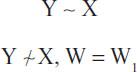
where ~ denotes association or correlation. Practically, this states that the overall association or correlation observed between the response variable (Y) and an explanatory variable (X) does not hold within strata defined by a third variable (W). Sometimes this is referred to as association reversal.⁴ These types of considerations overlap into issues regarding causation and conditional independence generally, but we do not examine those issues here.

Simpson’s paradox occurs both for continuous and discrete random variables in a similar manner. Here we give several basic examples with relevance to genetic studies examining expression through time or ordered stages of secondary variables.

Example 1

Consider a study examining a relationship of standardized gene expression differences between cases and controls at a specific loci y_i and dosage levels of a specific drug x_i. All subjects have been taking the treatment for at least 1 year. A secondary variable reflecting severity of oxidative stress (high/low) is suspected of affecting underlying epigenetic triggers (w_i). A simple linear model, y_i = β_o+β₁x_i+ε_i, is fitted to the overall data. It is obvious that the aggregated data can mislead, leaving undetected patterns within the strata and giving incorrect magnitude and sign to the coefficient of the regression. See Table 1 and Figure 1.

Table 1 Standardized gene expression differences and dosages with latent variable level Abbreviations: y, phenotypic response; x, dosage; W, secondary variable.

Figure 1 Gene expression differences across secondary variable levels.

Example 2

We assume here two time-ordered methylation triggers and examine the association between phenotype A (yes/no) and gene B, where expression beyond a given threshold is taken to indicate gene expression (yes/no). If time and degree of methylation are not accounted for, there is a possibility that we are aggregating gene expressions that may be distinct in terms of ordered expression and related functional impact and relevance. Categorical summaries are as susceptible to this as are continuous measures. Many early GWAS-related testing approaches did not account for time-ordering in expression data or the layered effects of epigenetic triggers. See Table 2.

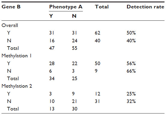Table 2 Association between gene and phenotype mediated by methylation Abbreviations: Y, yes; N, no.

Example 3

The potential for Simpson’s paradox extends to broader and more detailed correlation-based studies where clusters or networks of correlated gene expressions collected through time or according to the ordered levels of a secondary epigenetic or exposure variable are to be analyzed. These settings may also reflect aggregated data effects, with the resulting overall analysis being very different from the stratified analysis.

Here we create an empirical example, simulating a setting with standardized gene expression differences between cases and controls measured at five specific loci (x_1i, …, x_5i) with a related two-level epigenetic expression pattern (w_1i, w_2i), all measured in relation to a phenotypic continuous response y_i among cases. Twelve matched cases and controls are examined. Correlation matrices are obtained for (y_i, x_1i, …, x_5i) both overall and for levels (w_1i, w_2i). As can be observed, overall correlations and correlations within strata are not in agreement. See Table 3.

Table 3 Correlation patterns overall and within stratifications Note: *denotes significantly different from zero (Fisher z-test). Abbreviations: y, phenotypic response; x, loci expression; W, epigenetic level.

Without functional models that accurately model or reflect the series or network of gene expressions that underlie most developmental and maintained genetic processes, many gene expression correlation and empirically defined network studies require careful interpretation. As the number of genetic, epigenetic, and exposure levels relevant to the gene expression process increase, this type of aggregation effect may become more pronounced and difficult to detect.

Simulation studies

Data-dependent algorithms such as singular value decomposition and the many related clustering algorithms⁸ are prone to difficulty when there are multilayered data and limited functional data. In this setting, the simulation of various models and model structures may prove useful to understand potential models and related observed structures in the generated data.

To generate appropriately correlated or clustered datasets it is useful to consider a continuous setting and assume normality to begin. Modifications and extensions to more complex datasets can be developed directly. For example, to generate specific correlations corresponding to levels of a stratification variable, say with increasing levels of correlation, we can use a two-step approach, first generating a set of explanatory variables x_i and then generating the related response y_i. We then repeat this, increasing the correlations as we move across strata. An approach might be to generate a set of p explanatory variables x_i according to a multivariate normal distribution N_n(0, Σ), where we set the correlations ρ(x_i, x_j) =0.5^|i−j|. This will give a set of correlated explanatory variables subject to some random noise. We can then generate responses of various forms, including both highly correlated and less correlated response variables; response variables. For example with three explanatory variables we can simulate;

where c is a mean level of response. To define and simulate correlation levels across various strata we need only alter the value of c and the set of included x_i.

Latent variables

To limit the potential for Simpson’s paradox, the effects of latent variables can be modeled in a study either directly or via simulation or application of Bayesian methods with minimally informative priors. Typically, structural equation models are employed when secondary variables are thought to be relevant to the modeling of the response variable and its relationships to key variables in the data. In the genetic setting, such models under the name path analysis date from the 1930s, long before the availability of modern genomic data.

Path analysis

In genetics, the use of path analysis⁹ dates back to the work of Sewal Wright.⁷ The approach examines the various interrelated and independent sources of variation and correlation that must be parsed out in relation to their effect on a response of interest. A typical path analysis model can be expressed in terms of variables, measured or latent, that are thought to relate to a specific outcome or phenotype. For example, consider a setting where two epigenetic triggers are related to two gene expressions and two resulting phenotypes. In such a setting, a path diagram might look like that shown in Figure 2, where the correlations between variables are defined along each path. Note that not all values and variables can be directly modeled. Unknown correlations can be given values across a set of possibilities and the robustness of the overall correlation examined. To obtain the correlation between elements in the path diagram, we multiply the correlations of elements along the path of interest. If there are multiple paths connecting the two variables of interest, we sum the obtained correlations for each path to obtain the overall correlation of interest. Here, the correlation between epigenetic factor 1 and phenotype 1 is given by a₁₁ · b₁₁ + a₂₁ · b₂₁.

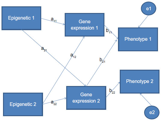Figure 2 Path analytic diagram for epigenetic triggers, related gene expressions, and resulting phenotypes.

Path analysis is theoretically based on a set of equations that incorporate all possible linkages among the variables. It allows researchers to visualize and organize the various potential relationships among the variables. Potential aggregation effects and Simpson’s paradox may occur here as well. Identified path analytic trees may differ in their patterns and structure from an overall, averaged tree. Object-oriented analysis¹⁰ has emerged in recent years providing more detailed statistical analysis of tree structures in data, often based on bootstrap resampling,¹¹ to achieve statistical significance of differences among tree structures.

Structural equation model

The model structure underlying the path analysis diagram can be generalized and applied much more broadly through a structural equation model. The approach has wide application in the social sciences, genetics,¹² and genetic twin studies where both genetic and environmental elements are to be assessed in a controlled setting, as well as any potential gene-environment interaction. Note that the idea of epigenetic signaling may correlate and overlap with the simpler concept of “environmental effect”. As a clearer view of epigenetic variables develops, reflecting a more nuanced gene-environmental interaction concept, researchers may wish to apply structural equation models more consistently.

In general, a structural equation model is typically composed of several equations. For the path analytic model considered above, the corresponding structural equation model can be interpreted from the diagram and written as:

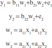
where the y_i variables define phenotypes of interest, w_i the gene expression levels, and x_i the epigenetic levels. Additional structure, such as correlated error terms, potential interaction, and nonlinearities may also be added into the equations. The errors e_i are assumed to be normally distributed. Note that the w_i variables exist within the overall context of the system of equations. Specific hypotheses can be examined, including specified correlations, and models can be fit to the data. Software for structural equation models includes the well known LISREL (version 9.1, 2013, Scientific Software International, Inc., Skokie, IL, USA) package.¹³

Discussion

It is essential to carefully model and interpret aggregate versus conditional or stratified effects in research disciplines applying statistical models, especially if primarily data analytic techniques are to be used. The idea of paradox here arises from limited experimental or study design and scientific understanding. In a rapidly moving science such as genetics or genomics, the chances that time as a variable, or other ordered epigenetic trigger variables related to gene expression are being aggregated inappropriately is high. Even simple empirical counter-examples show the need to carefully approach multilayered or time-ordered phenomena. The empirically driven methods underlying much gene expression-related cluster analysis are all technically susceptible to such aggregation effects. This, in addition to the file-drawer effect of unpublished negative results, should lead to careful assessments of results.

If the time or ordering aspect of gene expression is disregarded or unknown, or the epigenetic triggers have not yet been identified, comparisons across the genome using, for example, standard GWAS or clustering methods may be misleading. Recent work on the three-dimensional structure of chromosomes within cells³ suggests that the linear structure of current GWAS analysis may not be appropriate. This structure allows for a wide variety of gene sharing between chromosomes across widely disparate sections of various chromosomes as a natural occurrence, one that is unexpected if the GWAS analysis is viewed from a one-dimensional linear perspective.

The often massive size of expression data collections does not preclude application of the effects discussed here or other difficulties arising related to the design of experiments.¹⁴ In fact, the collapse of standard errors in such settings may make it more difficult to detect association reversal, as significance in general becomes difficult to interpret. The art of simulation is very useful in these settings to generate toy datasets that, with appropriate structures can be used to carefully assess and examine the relevance and stability of various potential models.

As functional and related hierarchical models become more commonly available for relating genotype to phenotype, and the related ordered expression of genes is better understood, more useful analytic models for many genetic phenomena will emerge and issues of aggregation and paradox should diminish.

Disclosure

The author has no conflicts of interest, financial or otherwise, to report in this work.

---

References

1.	Ptashne M. Epigenetics: core misconcept. Proc Natl Acad Sci U S A. 2013;110:7101–7103.
2.	ENCODE Project Consortium. Identification and analysis of functional elements in 1% of the human genome by the ENCODE pilot project. Nature. 2007;447:799–816.
3.	Tanizawa H, Iwasaki O, Tanaka A, et al. Mapping of long-range associations throughout the fission yeast genome reveals genome organization linked to transcriptional regulation. Nucleic Acids Res. 2010;38:8164–8177.
4.	Julious SA, Mullee MA. Confounding and Simpson’s paradox. BMJ. 1994;309:1480–1481.
5.	Samuels ML. Simpsons paradox and related phenomena. J Am Stat Assoc. 1993;88:81–88.
6.	Neale MC, Schmitt JE. Quantitative genetics and structural equation modeling in the age of modern neuroscience. In: Cannon T, editor. The Genetics of Cognitive Neuroscience Phenotypes. Proceedings of the 35th annual meeting of the Society for Neuroscience, November 12–16, 2005, Washington, DC, USA.
7.	Wright S. Correlation and causation. J Agric Res. 1921;20:557–585.
8.	Datta S, Datta S. Comparisons and validation of statistical clustering techniques for microarray gene expression data. Bioinformatics. 2003;19:459–466.
9.	Lleras C. Path analysis. In: Encyclopedia of Social Measurement. New York, NY, USA: Academy Press; 2005.
10.	Wang H, Marron JS. Object-oriented data analysis: sets of trees. Ann Stat. 2007;35:1849–1873.
11.	Holmes S. Bootstrapping phylogenetic trees: theory and methods. Stat Sci. 2003;18:241–255.
12.	Rosa GJ, Valente BD, de los Campos G, Wu XL, Gianola D, Silva MA. Inferring causal phenotype networks using structural equation models. Genet Sel Evol. 2011;43:6.
13.	LISREL 8.8. Skokie, IL, USA: Scientific Software International Inc; 2005.
14.	Lambert CG, Black LJ. Learning from our GWAS mistakes: from experimental design to scientific method. Biostatistics. 2012;13:195–203.