Efficacy of Government Responses to COVID-19 in Mediterranean Countries

Introduction

The new coronavirus disease (COVID-19) that began in Wuhan, China in December 2019, has spread quickly over the entire world.^1–4 The World Health Organization (WHO) declared that COVID-19 had advanced into a pandemic on March 11, 2020. The disease has culminated into larger chains of spread, resulting in widespread transmittal across the globe, affecting all continents.^5–7 Approximately 214 countries reported the number of confirmed coronavirus cases within a few weeks.^8,9 In the early stages of the outbreak, many governments tried containment strategies,^10,11 while the United Nations (UN) launched the Global Humanitarian Response Plan for the coronavirus pandemic.¹² However, case numbers skyrocketed, showing that it was no longer possible to contain the spread of the disease. Thus, some countries, including China, launched suppression strategies.^13,14 The daily increasing numbers of infections and deaths have led to quarantines, worldwide lockdowns, and other restrictions.⁸ The accelerating spread and the outcomes of the disease around the world have led people to panic, fear and anxiety.^15–17 In response, governments have enacted several economic and social measures and public health interventions.¹⁸ Governments intend to reduce the number of new infections and associated mortality, while also mitigating the potentially disastrous impact on the national health systems.¹⁹ Countries are implementing different combinations of various measures, with varying levels of stringency. Plans typically combine public health policies with mobility restrictions.²⁰ Although the approaches taken by national governments worldwide have varied widely,²¹ the measures adopted can be classified into five categories: movement restrictions, social distancing, lockdowns, public health measures, and social and economic measures.^22,23 Alfano and Ercolano¹ distinguished two principal types of policies: health policies aimed at strengthening hospital capacity, and policies, such as lockdown and social distancing measures, aimed at reducing viral transmission. Socio-economic policies aimed to reduce economic losses due to the halting of productive activities.^6,24–26 Policy measures were taken to protect economies, targeting both people and businesses, protecting both employment and the continuation of necessary economic activities.^18,27 The overall objective was to reduce coronavirus transmission in order to flatten the epidemic curve.²⁸ However, such measures also risk generating or exacerbating socio-economic problems such as inequitable distribution of harms due to the pandemic, and also due to the interventions themselves.^19,27 Successful governance hinges upon the use of information and relevant knowledge to prevent and control the epidemic, which underscores the need to improve the countries’ communicable disease governance capabilities and enhance the public health systems at large.²⁹

Government responses to the COVID-19 pandemic have been heterogeneous, however, around the world.³⁰ The effectiveness and the appropriateness of lockdown have been debated extensively, both for how well it contains the virus, and also for the economic and social costs incurred. In fact, countries are now facing new socio-economic situations that were not anticipated, with an unprecedented scale of impacts that it might take a long time for the world to recover, economically and societally.^12,18 Many scholars have argued that the consequences are actually playing out very much as predicted, and very much in line with the precedents of past pandemics. A complication of the response mechanism is whose advice was not heeded. For example, the USA government had pandemic predictions and preparation plans already in place, but they were ignored by the government in power at the time of the pandemic. Some countries considered tighter lockdowns to be a major factor in reducing contagion,¹³ initiating early social distancing measures and mandatory shutdown of nonessential businesses.^30,31 The argument is that shortening the crisis period would reduce the number of infections, and also decrease the duration of economic disruption.³² The WHO recommended that strict containment measures should be introduced in Italy as early as possible to push down the epidemic curve. Other countries considered that the outbreak could be contained without lockdown. Instead, they opted for a gradual approach based on awareness-raising plus penalties for contravening government instructions. They relied heavily on test-and-trace strategies.³¹ The idea was to keep as many people in work for as long as possible.^1,32 When trying to slow the epidemic’s spread, governments have opted for mitigation, ie flattening the epidemic curve, both to lighten the burden on health systems and also to improve social perception of the epidemic.¹¹ Most governments opted for social distancing, albeit to varying degrees, which include quarantine for regions with high case counts, travel restrictions, school closures, working from home, and the closure or restriction of restaurants, theatres, cinemas, and stadiums. Yet, a large fraction of the Italian population contravened the protective health measures.³³ In fact, Roma et al³³ highlighted that behavioral obedience to governments’ measures could be expected, given the psychological and social context. For instance, the predicted level of compliance depends on risk perception and public engagement. Also, at the beginning of the crisis, Tunisia recorded zero new infections for several days, bringing the total number of infections to the range of 1000 cases, of which about 800 were cured. The government thus considered that Tunisia had defeated the coronavirus, unlike the developed countries. On the other hand, the scientific committee recommended more vigilance and adherence to preventive measures in public spaces and shops so that the epidemiological situation would remain under control, and so that the results achieved by quarantine could be preserved. This would ensure zero new cases of infection for a period equal to twice the virus’s incubation period. But the borders were totally reopened without any precautionary measures as of June 27, and the pandemic’s suppression gave way to the virus’s return and rapid spread.

Atalan⁸ studied the effect of lockdown days on the spread of COVID-19 cases in 49 countries. He found that the lockdown—as one of the social isolation restrictions—limits the pandemic by significantly reducing infection. Varghese and Xu³⁰ found that government-driven social distancing measures reduced transmission in both Australia and New Zealand. Sebastiani et al²⁸ analyzed the impact of government measures in several Italian regions, finding that the earlier measures are taken in the epidemic’s evolution, the lower the total cumulative incidence achieved during that epidemic wave. In fact, after further restricting social interaction, mobility and non-vital economic activities, the daily number of new coronavirus cases in Italy stabilized towards the end of March, suggesting that the epidemic may have started to slow. The lag between the implementation of the government measures and the peaking of the “cumulative incidence” growth rate of the COVID-19 (the first signs of effectiveness) was found to be between 7 and 10 days. Saez et al¹¹ analyzed the effectiveness of the measures to be taken to mitigate the epidemic in Spain. After coronavirus case numbers skyrocketed, the Spanish government imposed social distancing. The measures managed to flatten the epidemic curve. In fact, the daily accumulation of cases decreased by more than three percentage points, and this reduction became greater as time passed.

This article aims to provide empirical evidence on the efficacy of policy measures taken by governments using panel data analysis and by addressing the question, How long do intervention measures take to become effective? Specifically, the aim is to analyze the efficacy of government measures against the COVID-19 pandemic, comparing the Mediterranean regions. In fact, despite the fragile health systems in the Eastern and Southern Mediterranean, characterized by weak disease surveillance and poor levels of public health preparedness, many countries took very early, bold and proactive steps to curtail the pandemic, and adopted various strategies for such prevention.³⁴ The same measures were taken later by the Northern Mediterranean countries where the public healthcare systems are considered more developed, and yielded better performance. Evidently, low-income and developing countries should adopt the policy guidelines of the developed countries.^27,35 In Italy and Spain, the first two epicenters of the pandemic in Europe,³⁷ policy measures were either partial (in the case of Italy) or decided upon and implemented too late (in the case of Spain).³⁶ The first cases in the Mediterranean region were detected at the end of January, and it started to spread exponentially a few weeks later. Over a period of only one week in late March, the number of confirmed cases nearly doubled in Italy and France, and in Spain, it almost tripled. Case increase rates remained high in April. Governments of countries hit later by coronavirus have, in principle, had more time to implement policy measures that had already proven effective in the countries that were hit first.³⁶ Meanwhile, new case counts from the southern and eastern Mediterranean countries are evidently lower than in Europe, even though their healthcare systems are weaker. Even though their first cases were registered in March, much later than in Europe, the governments of these countries took early and rapid national measures to contain contagion, ie when the case count was relatively low. They benefited and learned from the experiences of Western countries.

Methodology

We estimated the following equation:

(1)

Where is a country-specific effect, is a time-specific effect, and is an idiosyncratic error term. The variable is the daily number of infections in country c at time t, which is measured in days. This is modeled as a function of the total number of confirmed cases in country c on the previous day, . To limit bias in the number of detected cases, we use a long-duration panel covering the period from 22 January to 19 Jun 2020. The incubation period is estimated to be less than 14 days.^38–40 Equation 1 also includes a dummy variable that signals whether or not, on day t-k, there was a government measure against COVID-19 implemented in country c, ie the dummy signals which country had a government measure in place for k days, in order to control for when the policy was in effect. We set to 1 on the first day when a control policy is adopted (whether movement restrictions, social distancing, public health measures, governance and socioeconomic measures, or lockdown) and also on all subsequent days when that measure is in place. Thus, identifies the k days elapsed since the policy was implemented, enabling measurement of the policy’s effect on the number of new cases. The effect the government measures is not limited to coefficient but also depends on and is related to the number of confirmed cases, .

Since the effect of government measures in any given period is affected by the total number of infections detected in that period, it is necessary to account for interaction effects between variables to avoid biased estimations. We limit our analysis to the Mediterranean countries to avoid large regional differences, such as cultural factors, that may influence the evolution of the viral pandemic.

Procedures

For government measures in response to COVID-19, we relied on the Assessment Capacities Project (ACAPS)¹(¹See “https://www.acaps.org/covid19-government-measures-dataset” (accessed 20 Jun 2020).) data from “COVID-19: Government Measures” that inventories all such measures implemented by governments worldwide. We used the latest version available, updated on 18 Jun 2020 (which had been accessed on 20 June 2020). Government measures can be considered in five categories: social distancing, movement restrictions, public health measures, social and economic measures, and lockdowns. New coronavirus case counts were obtained from the John Hopkins University Center for Systems Science and Engineering (CSSE) COVID-19 repository⁴¹ in²(²See “https://github.com/CSSEGISandData/COVID-19”.) the latest version available, on 20 June 2020. It offers a daily estimate of the number of cases from 22 January to 19 June 2020.

We estimate the results for 15 Mediterranean countries: Spain, France, Italy, Croatia, Greece and Turkey along the southern European coast; Syria, Lebanon and Israel on the Levantine coast; Egypt, Tunisia, Algeria, and Morocco on the north African coast; and the island states of Malta and Cyprus within the Mediterranean Sea. We did not apply any inclusion and exclusion criteria to select the countries. For France, we exclude the overseas territories and limit our sample to the observed COVID-19 cases in the metropolitan territory.

Econometric Models

We estimate several regression models (from k=1 to k=26 days) for each one of the five measures. The shortcoming of using linear regressions with count-dependent variables is that the predicted values can be negative, and hence meaningless. However, as our objective is to determine whether government measures are important in explaining the response variable without estimating how much, we begin with the linear panel regressions only as starting points and afterward, we estimate the panel count data regressions.

Panel Regression Models

This section considers what estimation processes are best suited to long panel datasets where the time dimension is long, and the cross-sectional dimension is short. Panel data estimations allow consistent estimation of the effects of observed covariates, even if the outcome variable depends also on other explanatory variables or observables, and is correlated with the observed ones. In the panel random effects (RE) model, the country-specific effect, η_c, is assumed to be a random variable uncorrelated with the explanatory variables, ie . This can be tested using cluster-robust standard errors to allow for heteroscedasticity and serial correlation. Then, η_c can be left in the composite error term η_c where and , and the resulting serial correlation over time can be handled by generalized least squares (GLS) estimation.⁴² It should be noted that the number of new COVID-19 cases, at time t with respect to t-1 in a country c, is calculated as . Thus, RE could be inappropriate, in this case, because the differences may have negative serial correlations, which can cause problems. In the fixed effects (FE) model, the country-specific effect is a random variable that is allowed to be correlated with exogenous explanatory variables in any time period. FE is thought to be a more convincing model for estimating individual effects. Moreover, the regressors are themselves outcomes of choice processes, and likely to be correlated with countries’ preferences and abilities as captured by the unobserved effects .⁴³ The Fisher test is used to settle whether FE or simple pooled OLS better fits the panel data, while RE is explored with⁴⁴ Lagrange Multiplier (LM) test that contrasts the random effects with pooled OLS. It is common to perform a Hausman⁴⁵ test for the presence of country-specific FE, where the null hypothesis is that the RE model applies, ie that . Wooldridge⁴⁶ recommended performing a panel-robust version of the Hausman test that is consistent in the presence of cross-sectional dependence.

The hybrid and correlated random-effects approaches^46–51 are flexible modeling alternatives to standard fixed-effects and random-effects models, because they distinguish within and between-cluster effects and allow for the inclusion of level-two variables (cluster-invariant variables). They yield estimates of the level-one covariates that are unbiased by cluster-level unobserved heterogeneity, while allowing for level-two cluster-invariant covariates (see Bell et al).⁵² Note that the correlated random effects (CRE) and fixed-effects estimates are equivalent (that are the within-cluster effects). The CRE approach controls for the average level of the observed covariates, , when measuring their partial effect on the outcome variable .^43,46 The model can be expressed as: . In this model, . Including picks up the correlation between this covariate and the unobserved random effects. Rejecting the null hypothesis H₀: at a sufficiently low significance level implies rejection of the RE in favor of FE specification. Then, the assumption holds that there is no correlation between the level-one covariates and the level-two error .

Erroneously ignoring possible cross-sectional correlation of regression disturbances over time and between subjects can lead to biased inference. Specifically, standard fixed- and random-effects models can result in inconsistent estimators and in misleading inferences, depending on the correlation between the observed regressors and the unobserved source generating the cross-sectional dependence.⁵³ In the case of long panel data models, the standard approach is to estimate a system of seemingly unrelated regression equations (SURE) from different cross-sectional units, using generalized least squares (GLS) techniques.⁵⁴ Alternative approaches are used to handle the cross-sectional dependencies. Parks⁵⁵ proposed the feasible generalized least squares (FGLS) method to account for spatial and temporal dependence in the disturbances of time-series cross-section (TSCS) models, as well as for heteroscedasticity across panels.^56–58 As an alternative to the FGLS models, Beck and Katz⁵⁹ suggested the panel-corrected standard errors (PCSE) approach related to the linear TSCS models. The residuals are assumed to be heteroscedastic and contemporaneously correlated across panels, and the parameters are estimated by either OLS or Prais and Winsten⁶⁰ regression. The coefficients of the FGLS and PCSE models are close. Parameter estimation by the FGLS model is more efficient, but with the disadvantage that the standard error estimates are conditional upon the estimated disturbance covariance.⁵⁹ To address the shortness of these two models, Driscoll and Kraay⁶¹ proposed a nonparametric approach producing robust standard errors (RSE) for panel regressions with cross-sectional dependence (for more details, see Hoechle’s⁵³ Stata XTSCC module for calculating RSE for panels with cross-sectional dependence). The error structure is assumed to be possibly correlated between the panels, auto-correlated up to some lag, and heteroscedastic across panels. The standard errors for coefficients are estimated by pooled OLS/WLS, and within FE regression. These standard errors are robust to very general forms of temporal and spatial cross-sectional dependencies when the time dimension becomes large. For the choice between the pooled OLS and FE regression with Driscoll-Kraay standard errors, Hoechle⁵³ performed a Hausman-type test for FE that is robust to very general forms of cross-sectional and temporal dependence, following Wooldridge’s⁴⁶ suggestion for how to perform a panel-robust Hausman test.

Regression of Panel Count Data

Standard count models include Poisson and the negative binomial (NB) models.^62–65 The NB model, originally proposed by Hausman et al,⁶⁶ was thought that it allows two forms of heterogeneity: the NB-1 and NB-2 forms. In the cross-sectional case, the NB model fit better than the Poisson model only in terms of log-likelihoods because it effectively adds a parameter. Remember that the RE approach is intended with the long panel data, ie a large number of groups and relatively few time periods per group. But the conditional FE Poisson regression is fully robust to distributional mis-specifications as long as the conditional mean is correctly specified.^67–69 According to Wooldridge,⁷⁰ the fixed-effects negative binomial (FENB) approach suffers from some shortcomings and should “probably never be used”. In his Journal of Econometrics paper, Wooldridge⁷⁰ showed that, in fact, the model collapses to depend on only one heterogeneity parameter. The study of Allison and Waterman⁷¹ stated that

the conditional negative binomial model for panel data, proposed by Hausman, Hall, and Griliches,⁶⁶ is not a true fixed-effects method. This method does not in fact control for all stable covariates.

Wooldridge⁷⁰ showed that the FE Poisson estimators are completely robust to the failures of the Poisson assumptions as, for example, the violation of the assumption of equidispersion or the presence of an excessive number of zeros in the data. The FENB in the panel data case does not come close to nesting the Poisson assumptions unless the heterogeneity is zero. In this specification, consistent estimates are produced under relatively weak assumptions: only the conditional mean needs to be correctly specified, but the standard errors usually need adjustment to account for the over- or under-dispersion. Wooldridge⁷⁰ recommends avoiding the FENB, without the need to test for overdispersion, for three reasons: First, the FENB imposes a very specific overdispersion of the form (), where is the mean effect, and thus there is only one source of heterogeneity. However, the Poisson estimator allows any kind of variance–mean relationship (ie overdispersed, underdispersed or equidispersed). The variance and the mean can exhibit any of these, depending on the covariate values. The second reason is that the FENB imposes the conditional independence, but the serial correlation is not allowed. However, the FE Poisson allows any kind of serial correlation. Another key benefit is that the FE Poisson is robust to dependence over time—we just need to cluster the standard errors. Note also that the FENB model is not robust to the failure of any of its assumptions, and the time constant variables do not drop out in the FENB estimation. Third, the estimation of the FENB model often fails to converge, very likely because of the weird overdispersion it requires for every unit i in the cross-section.

Whether the conditional likelihood FE Poisson models or the generalized linear model (GLM) is best for count data depends on three factors: the nature of the research question, the link function, and the willingness of the researcher to accept low levels of bias.⁵² The problem we have with the fully robust FE Poisson estimator is that clustering may not be justified for small N and large T. Wooldridge recommends using pooled Poisson regression, including the groups’ dummy variables and time trends. We cannot really cluster in that case, but we can make the standard errors robust to the violations of the Poisson assumptions. The generalized estimating equation (GEE) approach^72,73 is used to produce more efficient and unbiased regression estimates.⁷⁴ It generalizes and extends the usual likelihood equation for the GLM by including the covariance matrix of the responses.⁷⁵ GEE regression requires the specifications of the dependent variable distribution, the link function to be used, and the within-group correlation structure of the response variable.⁷⁴ One should carefully consider the parametrization of the working correlation matrix since including the correct specification of the correlation form within the dependent variables increases the efficiency of the estimates.^74–76 However, the model is robust to mis-specification of correlation structure because the estimated regression parameters remain consistent. Therefore, the efficiency gains from accurate specification of the structure are usually slight.^72,74 GEE model provides consistent estimates of the parameters when the mean is correctly specified, even if the within-group correlation structure is not correctly specified.⁷⁷ In fact, consistent estimates of the standard errors can be obtained via the robust covariance matrix that adjusts for efficiency losses due to possible misapplication of the variance function. Note that the GEE models are fairly robust against the wrong choice of correlation matrix, particularly in our case with a large sample size. The parameters and standard errors can be estimated consistently with the Huber–White “sandwich” estimator^78,79 even if the correlations within group are not as hypothesized by the specified correlation structure.^80,81 Zeger et al⁸² used the three different correlation assumptions (repeated observations uncorrelated, exchangeable correlation, and stationary correlation) to demonstrate that both the estimates and their respective standard deviations show little dependence on the choice of the correlation matrix, despite the presence of substantial correlation among the data.

Statistical Analyses

We start empirically investigating the heteroscedasticity, serial correlation and contemporaneous correlation of the disturbance term across cross-sectional units. Table 1 shows the different statistical tests for each of the five categories of government measure against COVID-19. FE models are tested by the F-test, , that all (the alternative hypothesis is that at least one parameter is not zero), while the RE models are examined by Breusch and Pagan’s⁴⁴ Lagrange multiplier (LM) test that contrasts the RE with pooled OLS. The LM test examines whether the country-specific variance components are zeros, H₀: , with the LM statistic following the distribution. The obtained p-values are small enough (at the p≤0.001 level) to reject the null hypothesis in either test. Thus, the FE and RE models are preferred over the pooled OLS model for all the government measures except that, for the governance and socio-economic measure, the LM test is statistically significant. The standard Hausman test of the FE models and Wooldridge’s⁴⁶ auxiliary regression for the panel-robust Hausman test, F (3, 14), in the presence of cross-sectional dependence is statistically significant indicating the presence of country-specific FE. The null hypothesis that the countries’ effects are uncorrelated with the other regressors is rejected, and thus the RE models are not favored over their FE counterpart. However, the statistical inference could be invalid in the presence of cross-sectional dependence. Breusch–Pagan LM tests indicate the presence of cross-sectional autocorrelation in FE. In fact, in the LM test of independence, H₀ is rejected so the correlation of different countries is significant. We perform, then, the robust Hausman test with Driscoll and Kraay standard errors.⁵³ The obtained Fisher statistics, F (3, 14), are statistically non-significant. Thus, the standard FE and RE models can result in inconsistent estimators and in misleading inference, depending on the correlation between the observed regressors and the unobserved source generating the cross-sectional dependence.⁵³ We also perform a modified Wald test to detect the existence of group-wise heteroscedasticity in the residuals of the FE regressions.^56,83 Under the null hypothesis, the variance of the error terms is the same for all countries: H₀: for all . The results lead to a strong rejection of the null hypothesis for p≤0.001. So, we conclude that heteroscedasticity is present.

Table 1 Estimation Strategies for the Complete Sample: Model Choice

We also estimated the FGLS and PCSE models (see columns 2 and 3 of Table 2). Then, the nonparametric approach of Driscoll and Kraay⁶¹ is used to address the shortness of these two models by producing RSE for panel regressions with cross-sectional dependence. In fact, our error structure is found to be possibly correlated between the panels, auto-correlated up to some lag, and heteroscedastic across panels. This is revealed in the statistically insignificant result of Wooldridge’s⁴⁶ serial autocorrelation test, where the hypothesis H₀: no first-order autocorrelation is not rejected, and thus there is no indication of a common first-order correlation (see Table 1). On the basis of these results, we choose Driscoll and Kraay’s⁶¹ method of producing heteroscedasticity, autocorrelation, and panel correlation consistent robust standard errors.

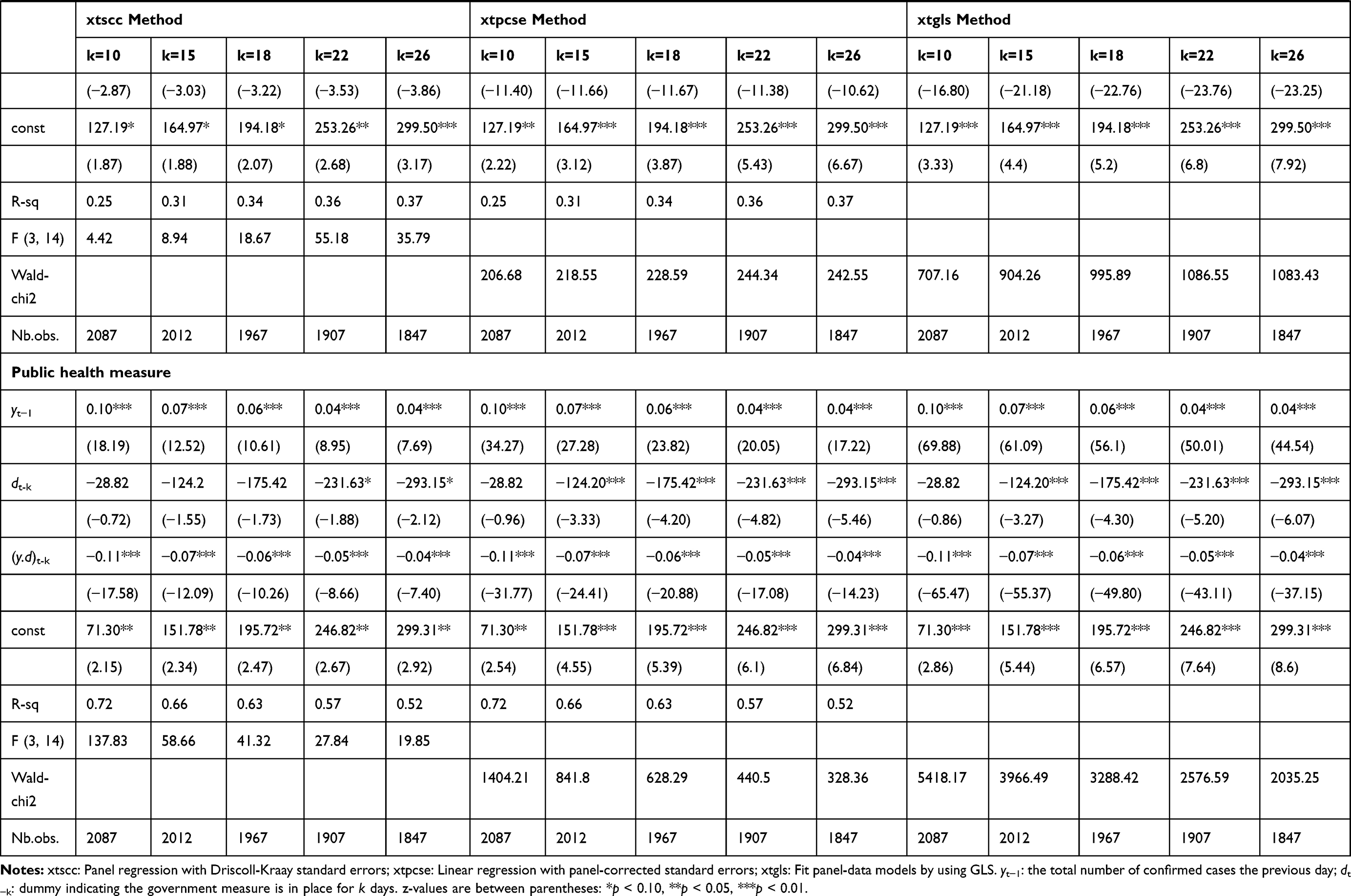Table 2 Robustness Checks

Results

Table 3 shows the results of the panel regressions with Driscoll–Kraay standard errors.³(³The robustness check of our selected estimation method is presented in Table 2. We estimated the panel regression model with Driscoll-Kraay standard (XTSCC), the linear regression with panel-corrected standard errors (PCSE), and the feasible generalized least squares (FGLS). The coefficients are closed.) There are, as expected, positive and statistically significant coefficients , suggesting that the more infection cases reported on previous days, the more new cases of the coronavirus there will be today. The number of detected viral new cases depends on both the total number of infections, and also the government measures already implemented. The effects of these two variables are related. We observe that the effect of the dummy variable is significantly positive over 8 days for the lockdown measure, and over 6 days for the other measures (social distancing, movement restrictions, …). We can also see that the benefits of government measures increase exponentially with the passing of days. These effects fall to statistical non-significance 9 days after the start of lockdown; 7 days after the start of social distancing and movement restriction measures. The coefficients become negative and significant after three weeks, suggesting a net benefit in having implemented the measures. Their magnitudes and statistical significance keep growing with an apparently exponential trend. In fact, the effect of the variable d will be negative after 22 days of lockdowns, and 21 days after each of the other implemented measures such as social distancing and movement restrictions. Estimates on the complete sample are reported in Figure 1 where the coefficients of the government measure dummies are computed from the date of implementation to 26 days after. We plot the coefficient for the health policies aimed at strengthening the capacity of the hospital systems and the policies aimed at reducing the viral transmission, such as lockdowns, social distancing and movement restriction measures.

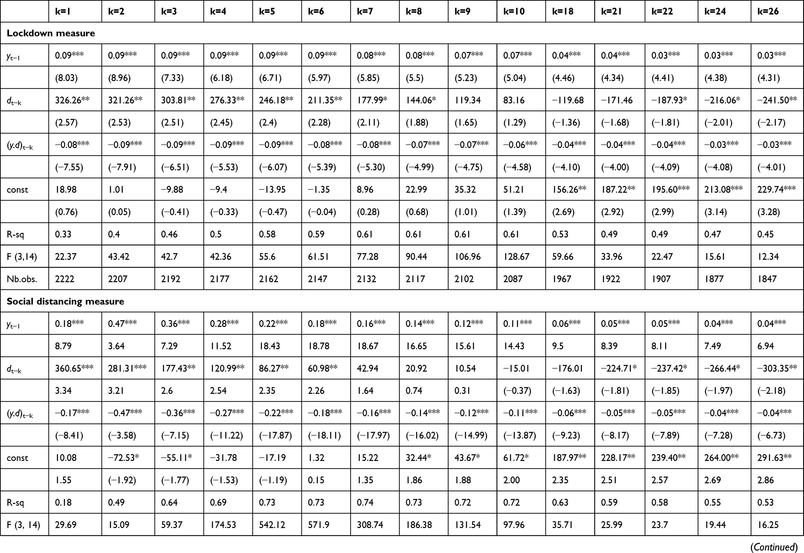Table 3 Panel Regression with Driscoll–Kraay Standard Errors (for the Complete Sample)

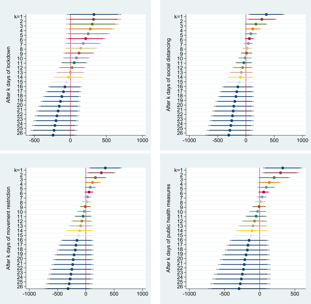Figure 1 Coefficients of government measure dummies for the complete sample.

Interestingly, when we account for the total number of infection cases on previous days (t-k) we notice that the government measures may be effective from the very first day of implementation. After estimating the parameters for several days (k days after the policy implementation), we determine, for each k, the number of total COVID-19 cases, , verifying (negative effects on the new confirmed cases) for the significantly positive coefficients . Figure 2 illustrates results calculated for the positive and statistically significant coefficients. Each point on the colored area corresponds to a negative effect on the number of new detected infections, ie a benefit due to the government measures. We can say that, after a week (more precisely, 8 days for lockdown or 6 days for the other four measures), the benefits of the government measures are related to the total number of COVID-19 cases confirmed on previous days. For example, after two days of lockdown, the net effect is negative and statistically significant if the total number of infections is less than 3695 on average, ie the spread of the virus is not already advanced. After nine days of lockdown, the effect of the total number of infections on the observed new cases will be reduced. The same remark concerns the other measures that governments take. Thus, the net effects of government measures can be divided into three phases: the first phase is within 9 days for lockdown, and within 7 days for the other measures. During this phase, benefits are not guaranteed when the total number of contamination cases is lower than the values corresponding to the points on the colored areas in Figure 2 for lockdown, social distancing, movement restrictions and public health measures. The second phase runs to the end of three weeks, and entails indirect benefits from each measure. During this second phase, the effects of the government dummy variables, d are statistically non-significant until 22 days after lockdown, and until 21 days after implementing social distancing, movement restriction, public health, and governance and socio-economic measures. The coefficients are statistically non-significant, and we observe only indirect effects revealed in the negative and significant signs of the interaction terms in the regression models. This means that the effect of the total confirmed cases, detected previous days, on the new confirmed infections may be reduced by the implementation of government measures. In the third phase, which begins three weeks after implementation, we observe the negative effects of government measures on the number of the confirmed viral cases, ie the direct benefits are observed (the coefficients become negative and statistically significant). For instance, lockdowns have negative and statistically significant coefficients, suggesting that countries that implemented the lockdown measures have fewer new cases than countries that did not. Figure 2 shows that, from the first week, lockdown with tighter restrictions is a major factor in reducing the contagion.¹³

Figure 2 Estimated cases verifying for the complete sample.

Thus, the spread of the coronavirus can be significantly reduced by preventive restrictions. The earlier measures are taken in relation to the stage of the epidemic, the lower the total cumulative incidence achieved during that epidemic wave. We show that the government measures can begin to take effect even in the first few days. This observation aligns with Sebastiani et al’s²⁸ findings that the time lag between the implementation of the government measures and the peaking of the “cumulative incidence” growth rate of COVID-19 (the first signs of effectiveness) was between 7 and 10 days. Containment measures should hence be introduced as early as possible to flatten the epidemic curve. Governments of countries hit later by coronavirus have, in principle, more time to implement policy measures that already proved effective in the countries already hit.

Our dependent variable is characterized by a large range of count values. The problem we have with the fully robust FE Poisson estimator is that clustering may not be justified for small N and large T. Thus, we fit population-averaged panel-data models using a GEE approach that allows for the heteroscedasticity and the specification of the within-group correlation structure for the panels. We note that the estimated parameters differ depending on what within-group correlation structure we choose. However, we find a large difference between the “independent” and “exchangeable” estimates, which indicate a failure of strict exogeneity. A goodness-of-fit test cannot help resolve this issue because it does not care about the exogeneity of the explanatory variables. Thus, we estimate a Poisson model with the continuous endogenous covariates frequently used to model nonnegative outcome variables. We use the two-step generalized method of moments (GMM) estimation procedure^46,62,84,85 where the variable is allowed to be instrumented by exogenous variables. To allow for heteroscedasticity of the errors, we use clustered robust standard errors to account for the correlation for groups of observations within clusters. The results confirm our findings of the non-discrete trajectory of the effects of government measures. In fact, the same three government intervention effect phases also emerge from this analysis.

Silva and Tenreyro^68,69 showed that maximum likelihood estimates (MLEs) for the Poisson regression may not exist for some data configurations. As a result, estimation algorithms may not be able to converge, or may converge to incorrect estimates. For this, we estimate the Poisson pseudo-likelihood regressions with multiway fixed effects, as described by Correia et al,^86,87 which are particularly useful in models with positive values, but without having to explicitly specify a distribution for the dependent variable. They lead to consistent estimates in the presence of heteroscedasticity, unlike the log-linearized models fitted by OLS.⁶⁷ The Poisson regression by the pseudo-maximum likelihood (PPML) method of Silva and Tenreyro⁶⁸ gives the same results. The estimation methods paint a very similar picture of the trajectory of the effects of government measures.

Table 4 shows the results of estimation of the Poisson pseudo-likelihood regression with high-dimensional fixed effects for the complete sample. The results are similar to those from the Driscoll–Kraay standard errors approach, which corrects for heteroscedasticity and auto-correlation, with shifts of 2 and 3 days, on average. Note that the interpretation of the parameters is not the same. Here, we should look at the partial effects of a change in the covariates on the modeled conditional expectation function because the model is nonlinear. The net effects of the government’s measures are shown, divided into three phases. The first phase runs for 6 days from the initial implementation of a government measure (lockdown, social distancing, movement restriction or public health measures). The coefficients are positive and statistically significant and the benefits are not guaranteed except when the total number of contamination cases (at day t-k) is lower than a certain value, verifying that . The second phase corresponds the period between one and three weeks when we found an indirect benefit of each measure. The effects of the government measure dummy variables, , are statistically non-significant for fewer than 18 days after lockdowns, fewer than 22 days after a social distancing measure, fewer than 21 days after a movement restriction measure, fewer than 24 days after a public health measure, and fewer than 23 days after a governance and socio-economic measure. In this phase, the coefficients are statistically non-significant and we observe only the indirect effects revealed in the negative and significant signs of the interaction terms in the regression models. After this phase ends, the negative and significant effects of the government measures are observed, indicating the direct benefits (the coefficients become negative and statistically significant).

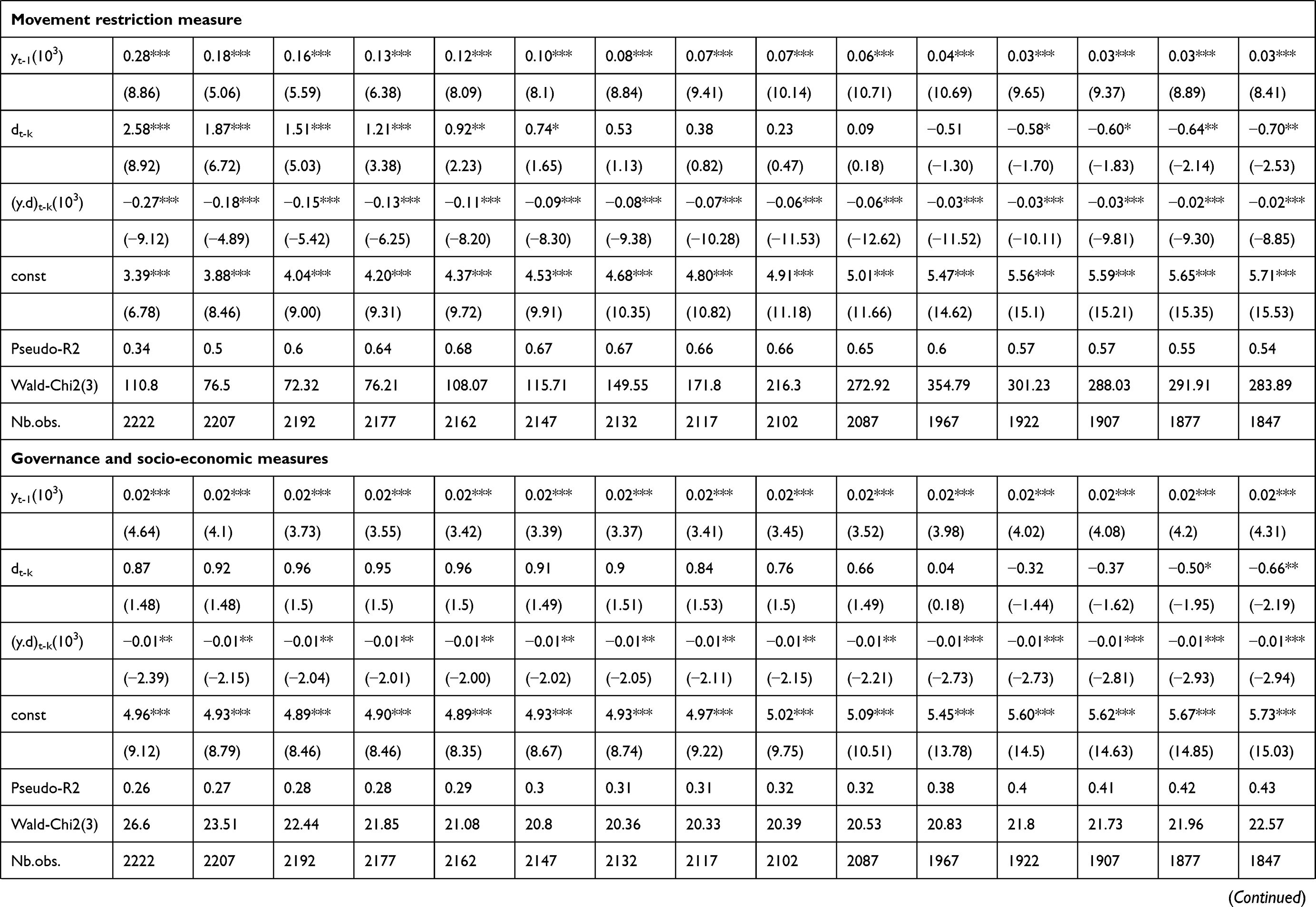Table 4 Poisson Pseudo likelihood Regression with Multiple Levels of Fixed Effects (for the Complete Sample)

Discussion

Among previous researches, Sebastiani et al²⁸ found that the time lag between the implementation of the government measures and the peaking of “cumulative incidence” growth rate (the first signs of effectiveness) was approximately 7 to 10 days. Alfano and Ercolano¹ show that lockdown is effective in reducing the number of new COVID-19 cases in countries that implement it, compared with countries that do not. This is especially true around 10 days after the implementation, and its efficacy continues to grow up to 20 days after implementation. Note that, in lockdown, all non-essential services and production are closed, and people cannot leave their houses apart for specific reasons that they must communicate to the authorities (full lockdown) or, for which they need to obtain a roaming license (partial lockdown). Social distancing measures consist of limiting public gatherings, canceling public events, closing schools, suspending social visits, etc. Movement restrictions entail additional health/documentation requirements upon arrival in a country, suspension of international flights, closure of land or sea borders, visa restrictions limiting specific nationalities from entering the country, or adding visa restrictions that did not exist before, etc. Public health measures may entail self-quarantine or isolation time upon arrival in a country—whether for all arrivals, arrivals experiencing symptoms, or arrivals who have been in touch with confirmed COVID-19 cases, health screenings and body temperature controls in airports and at border crossings, strengthening of the public health system. Strengthening the public health system could entail hiring more medical personnel, building new hospitals and medical centers or expanding current ones, requiring that protective gear be worn in public, psychological assistance. On the social front, authorities have implemented psychological assistance measures for the patients and their families, as well as for people in quarantine or lockdown. For the governance and socio-economic measures, authorities have taken economic measures in order to mitigate the impact that other restrictions have on the economy. To mitigate impacts on society, emergency administrative structures have been activated or established, such as Emergency Response committees, etc., in order to coordinate the response and/or decide on measures and/or monitor implementation, military deployment to support medical operations and ensure compliance with the measures. Product imports/exports have been limited and, in cases, authorities have declared a state of emergency. States of emergency are usually effected in order to permit other measures that are disallowed by constitution under normal conditions. States of emergency may include a state of necessity, exceptional state, or state of public health emergency.

We observe a slightly different situation in the European subsample with high numbers of daily confirmed COVID-19 cases (Italy, France, Spain and Turkey). The effects of government measures become negative after four weeks. This can be explained by the fact that the spread of the virus was already advanced. It is worth noting that, in Italy, the first registered infection case occurred on January 30th. From then to 15 March 2020, the number of confirmed cases increased exponentially, reaching 24,747 people, with 2335 reported recoveries and 1, 809 deaths. Even if Italy has one of the best public healthcare systems in the western world, the shared volume of infections, particularly those requiring intensive hospital care, has seriously challenged the system. This is a healthcare system that benefitted from general government expenditure equating to 8.84% of GDP in 2017 despite low GDP growth rates (0.3% in 2019).³⁷ Preventive measures were not implemented until after WHO’s international declaration of emergency. The strongest containment measures began on 21st February in selected “red zones,” and then extended throughout the north of the country on 22nd March all non-essential economic activities were closed. At the same, the coronavirus started to spread in Spain at the beginning of March 2020, reaching 7798 cases on the 15th March, with 517 recoveries and 289 reported deaths. In terms of infrastructure, the Spanish healthcare system is considered relatively developed. However, the very first measures came into force mid-March, both to limit viral spread and also to mitigate economic impact. In mid-March 2020, Italy and Spain both adopted social distancing measures, 13 days after the outbreak had started its exponential growth. By 12th May, Spain was the worst affected Mediterranean country, with over 224,000 confirmed cases, followed by Italy with 219,070 cases.

Conclusion

In this paper, we sought to provide empirical evidence for the effectiveness of Mediterranean government policy measures (lockdowns, social distancing, movement restrictions, public health measures, and governance and socio-economic measures) in response to the COVID-19 pandemic. We focused on how long these measures took to become effective, using longitudinal linear and count data regression models. We estimated the results for 15 Mediterranean countries—Spain, France, Italy, Croatia, Greece and Turkey (south European coast); Syria, Lebanon and Israel (Levantine coast); Egypt, Tunisia, Algeria, and Morocco (north African coast); and Malta and Cyprus within the Mediterranean Sea. For France, we excluded the overseas territories, and limited our sample to the observed COVID-19 cases in the metropolitan territory. The analysis is limited to the Mediterranean countries to avoid regional differences, such as cultural factors, that may influence the evolution of the viral pandemic. Though there are some commonality and connectedness around the Mediterranean, we may still be concerned about the socio-economic differences, government–civilian–military relationships (eg civilian compliance levels), health systems, and even physical features (climate, urban–rural structure, internal mobility) between the countries. The comparison of the different regions will be in a further paper.

Different estimation methods were used to investigate the heteroscedasticity, serial correlation and contemporaneous correlation of the disturbance term across the cross-section of countries. Our different estimation methods paint very similar pictures of the efficacy trajectory of governments’ measures. The benefits of governments’ measures increase exponentially as time passes, passing through three phases. In the first week, the benefits of government measures are not guaranteed unless the total number of contamination cases is less than certain values, ie unless the spread of the virus is not already advanced. In the second phase, indirect effects are revealed. In the third phase, which begins three weeks after implementation, we observe the negative effects of the government measures on the number of the new confirmed viral cases and, thus, direct net benefits are observed. The earlier the measures are taken in relation to the stage of the epidemic, the lower the total cumulative incidence achieved during that epidemic wave.

However, due to lack of information, the study did not take into account the incongruities in how the public undertook the protective health practices that governments asked of them. In fact, the study was done early at the first phase of the pandemic, on June 2020, at which time inconsistent public behavior could be expected, given the variation of psychological and social factors according to risk perception and civic engagement. Also, there are no comparator countries in which no government measures were in place.

Government responses to COVID-19 had, and have, various impacts. Thus, we relied on a five-category taxonomy: lockdowns, social distancing, movement restrictions, public health measures, and governance and socio-economic measures.

Our study contributes to the debate regarding the need for government policies, and it may contribute specifically to the debate on strategies and mitigation measures by using movement restrictions, public health measures, social distancing, lockdowns, and socioeconomic measures.

For instance, the governance and socio-economic measures may be represented in economic measures taken in order to mitigate the impact that other restrictions have on the economy and society, and in the implementation of emergency response committees and administrative structures for good response coordination, deciding on measures, and/or monitoring their implementation. Governance also consists of declaring a state of emergency, which includes a state of public health emergency, to permit emergency actions.

The net effects of government measures manifest in three phases, and each country can develop a strategy appropriate to its economic capabilities. Yet, the paper has not compared countries across a broad spectrum of GDP, health infrastructure and access to health care, due to the constraints of time and information availability.

References

1. Alfano V, Ercolano S. The efficacy of lockdown against COVID-19: a cross-country panel analysis. Appl Health Econ Health Policy. 2020;18:509–517. doi:10.1007/s40258-020-00596-3
2. Shah AUM, Safri SNA, Thevadas R, et al. COVID-19 outbreak in Malaysia: actions taken by the Malaysian government. Int J Infect Dis. 2020;97:108–116. doi:10.1016/j.ijid.2020.05.093
3. Saglietto A, D’Ascenzo F, Zoccai GB, De Ferrari GM. COVID-19 in Europe: the Italian lesson. Lancet. 2020;395(10230):1110–1111. doi:10.1016/S0140-6736(20)30690-5
4. Wu F, Zhao S, Yu B, et al. A new coronavirus associated with human respiratory disease in China. Nature. 2020;579(7798):265–269. doi:10.1038/s41586-020-2008-3
5. Gates B. Responding to Covid-19: a once-in-a-century pandemic? N Engl J Med. 2020;382(18):1677–1679. doi:10.1056/NEJMp2003762
6. Anderson RM, Heesterbeek H, Klinkenberg D, Hollingsworth TD. How will country-based mitigation measures influence the course of the COVID-19 epidemic? Lancet. 2020;395(10228):931–934. doi:10.1016/S0140-6736(20)30567-5
7. Shammi M, Bodrud-Doza M, Islam ARMT, Rahman MM. COVID-19 pandemic, socioeconomic crisis and human stress in resource-limited settings: a case from Bangladesh. Heliyon. 2020;6(5):e04063. doi:10.1016/j.heliyon.2020.e04063
8. Atalan A. Is the lockdown important to prevent the COVID-9 pandemic? Effects on psychology, environment and economy-perspective. Ann Med Surg. 2020;56:38–42. doi:10.1016/j.amsu.2020.06.010
9. Chakraborty I, Maity P. COVID-19 outbreak: migration, effects on society, global environment and prevention. Sci Total Environ. 2020;728:138882. doi:10.1016/j.scitotenv.2020.138882
10. Legido-Quigley H, Asgari N, Teo YY, et al. Are high-performing health systems resilient against the COVID-19 epidemic? Lancet. 2020;395(10227):848–850. doi:10.1016/S0140-6736(20)30551-1
11. Saez M, Tobias A, Varga D, Barcelo MA. Effectiveness of the measures to flatten the epidemic curve of COVID-19. The case of Spain. Sci Total Environ. 2020;727:138761. doi:10.1016/j.scitotenv.2020.138761
12. Djalante R, Lassa J, Setiamarga D, et al. Review and analysis of current responses to COVID-19 in Indonesia: period of January to March 2020. Prog Disaster Sci. 2020;6:100091. doi:10.1016/j.pdisas.2020.100091
13. Kraemer MUG, Yang CH, Gutierrez B, et al. The effect of human mobility and control measures on the COVID-19 epidemic in China. Science. 2020;368(6490):493–497. doi:10.1126/science.abb4218
14. Zhang S, Wang Z, Chang R, et al. COVID-19 containment: china provides important lessons for global response. Front Med. 2020;14(2):215–219. doi:10.1007/s11684-020-0766-9
15. Ahorsu DK, Lin CY, Imani V, Saffari M, Griffiths MD, Pakpour AH. The Fear of COVID- 19 Scale: development and Initial Validation. Int J Ment Health Addict. 2020;1–9. doi:10.1007/s11469-020-00270-8
16. Duan L, Zhu G. Psychological interventions for people affected by the COVID-19 epidemic. Lancet Psychiatry. 2020;7(4):300–302. doi:10.1016/S2215-0366(20)30073-0
17. Wang G, Zhang Y, Zhao J, Zhang J, Jiang F. Mitigate the effects of home confinement on children during the COVID-19 outbreak. Lancet. 2020;395(10228):945–947. doi:10.1016/S0140-6736(20)30547-X
18. Kuckertz A, Brändle L, Gaudig A, et al. Startups in times of crisis - A rapid response to the COVID-19 pandemic. J Bus Ventur Insights. 2020;13:e00169. doi:10.1016/j.jbvi.2020.e00169
19. Glover RE, van Schalkwyk MC, Akl EA, et al. A framework for identifying and mitigating the equity harms of COVID-19 policy interventions. J Clin Epidemiol. 2020;128:35–48. doi:10.1016/j.jclinepi.2020.06.004
20. Akim A, Ayivodji F. Interaction effect of lockdown with economic and fiscal measures against COVID-19 on social-distancing compliance: evidence from Africa. SSRN Electron J. 2020. SSRN-3621693. doi:10.2139/ssrn.3621693
21. Piguillem F, Shi L The optimal COVID-19 quarantine and testing policies. CEPR Discussion Paper No. DP14613; 2020.
22. ACAPS. COVID-19 government measures dataset. Geneva: The Assessment Capacities Project; 2020. Available from: https://www.acaps.org/covid19-government-measures-dataset.
23. Wahba K. Assessing the intervention’s effectiveness and health system efficiency during COVID-19 crisis using a signal-to-noise ratio index. medRxiv. 2020. doi:10.1101/2020.05.07.20094334
24. Atkeson A. What Will Be the Economic Impact of COVID-19 in the US? Rough Estimates of Disease Scenarios. National Bureau of Economic Research; 2020:w26867. doi:10.3386/w26867
25. Eichenbaum M, Rebelo S, Trabandt M. The Macroeconomics of Epidemics. National Bureau of Economic Research; March, 2020:w26882. doi:10.3386/w26882
26. Qiu Y, Chen X, Shi W. Impacts of social and economic factors on the transmission of coronavirus disease 2019 (COVID-19) in China. J Popul Econ. 2020;33:1127–1172. doi:10.1007/s00148-020-00778-2
27. Loayza NV. Costs and Trade-Offs in the Fight Against the COVID-19 Pandemic: A Developing Country Perspective. Washington, DC: World Bank Research and Policy Briefs; 2020. No.148535.
28. Sebastiani G, Massa M, Riboli E. Covid-19 epidemic in Italy: evolution, projections and impact of government measures. Eur J Epidemiol. 2020;35(4):341–345. doi:10.1007/s10654-020-00631-6
29. Gu E, Li L. Crippled community governance and suppressed scientific/professional communities: a critical assessment of failed early warning for the COVID-19 outbreak in China. J Chin Gov. 2020;5(2):160–177. doi:10.1080/23812346.2020.1740468
30. Varghese C, Xu W. Quantifying what could have been- The impact of the Australian and New Zealand governments’ response to COVID-19. Infect Dis Health. 2020;25(4):242–244. doi:10.1016/j.idh.2020.05.003
31. Cohen J, Kupferschmidt K. Countries test tactics in ‘war’ against COVID-19. Science. 2020;367(6484):1287–1288. doi:10.1126/science.367.6484.1287
32. Karnon J. A simple decision analysis of a mandatory lockdown response to the COVID- 19 pandemic. Appl Health Econ Health Policy. 2020;18(3):329–331. doi:10.1007/s40258-020-00581-w
33. Roma P, Monaro M, Muzi L, et al. How to improve compliance with protective health measures during the COVID-19 outbreak: testing a moderated mediation model and machine learning algorithms. Int J Environ Res Public Health. 2020;17(19):7252. doi:10.3390/ijerph17197252
34. Al-Tawfiq JA, Memish ZA. COVID-19 in the Eastern Mediterranean Region and Saudi Arabia: prevention and therapeutic strategies. Int J Antimicrob Agents. 2020;55(5):105968. doi:10.1016/j.ijantimicag.2020.105968
35. Barnett-Howell Z, Mobarak AM Should Low-income countries impose the same social distancing guidelines as Europe and North America to halt the spread of COVID-19? New Haven, CT: Yale School of Management; 2020.
36. Ayadi R Time for a decisive coordinated response to a costly global COVID- 19 systemic crisis: towards a Global Resilient System. EMEA - Euro-Mediterranean Economists Association; 2020.
37. Ayadi R, Ali SA, Alshyab N, et al. Covid-19 in the Mediterranean and Africa: diagnosis, policy responses, preliminary assessment and way forward. Euro-Mediterranean Economists Association; 2020.
38. Lauer SA, Grantz KH, Bi Q, et al. The incubation period of Coronavirus disease 2019 (COVID-19) from publicly reported confirmed cases: estimation and application. Ann Intern Med. 2020;172(9):577–582. doi:10.7326/M20-0504
39. Li Q, Guan X, Wu P, et al. Early transmission dynamics in Wuhan, China, of novel coronavirus–infected pneumonia. N Engl J Med. 2020;382(13):1199–1207. doi:10.1056/NEJMoa2001316
40. Linton NM, Kobayashi T, Yang Y, et al. Incubation period and other epidemiological characteristics of 2019 novel coronavirus infections with right truncation: a statistical analysis of publicly available case data. J Clin Med. 2020;9(2):538. doi:10.3390/jcm9020538
41. Dong E, Du H, Gardner L. An interactive web-based dashboard to track COVID-19 in real time. Lancet Infect Dis. 2020;20(5):533–534. doi:10.1016/S1473-3099(20)30120-1
42. Cameron AC, Trivedi PK. Micro-Econometrics Using Stata. College Station, Tex: Stata Press; 2009.
43. Wooldridge JM. Introductory Econometrics: A Modern Approach.
44. Breusch TS, Pagan AR. The Lagrange Multiplier Test and its applications to model specification in econometrics. Rev Econ Stud. 1980;47(1):239–253. doi:10.2307/2297111
45. Hausman JA. Specification tests in econometrics. Econometrica. 1978;46(6):1251–1271. doi:10.2307/1913827
46. Wooldridge JM. Econometric Analysis of Cross Section and Panel Data. MIT press; 2010.
47. Mundlak Y. On the pooling of time series and cross section data. Econometrica. 1978;46(1):69–85. doi:10.2307/1913646
48. Allison P. Fixed Effects Regression Models. Los Angeles: SAGE; 2009.
49. Schunck R. Within and between estimates in random-effects models: advantages and drawbacks of correlated random effects and hybrid models. Stata J. 2013;13(1):65–76. doi:10.1177/1536867X1301300105
50. Schunck R, Perales F. Within- and between-cluster effects in generalized linear mixed models: a discussion of approaches and the Xthybrid command. Stata J. 2017;17(1):89–115. doi:10.1177/1536867X1701700106
51. Wooldridge JM. Correlated random effects models with unbalanced panels. J Econom. 2019;211(1):137–150. doi:10.1016/j.jeconom.2018.12.010
52. Bell A, Fairbrother M, Jones K. Fixed and random effects models: making an informed choice. Qual Quant. 2019;53(2):1051–1074. doi:10.1007/s11135-018-0802-x
53. Hoechle D. Robust standard errors for panel regressions with cross-sectional dependence. Stata J. 2007;7(3):281–312. doi:10.1177/1536867X0700700301
54. Zellner A. An efficient method of estimating seemingly unrelated regressions and tests for aggregation bias. J Am Stat Assoc. 1962;57(298):348–368. doi:10.1080/01621459.1962.10480664
55. Parks RW. Efficient estimation of a system of regression equations when disturbances are both serially and contemporaneously correlated. J Am Stat Assoc. 1967;62(318):500–509. doi:10.1080/01621459.1967.10482923
56. Greene W. Econometric Analysis. New York, NY: Prentice Hall; 2018.
57. Maddala GS, Lahiri K. Introduction to Econometrics. A john Wiley and Sons, Ltd, publication; 2009.
58. Kmenta J. Elements of Econometrics. New York: Macmillan; 1986.
59. Beck N, Katz JN. What to do (and Not to Do) with time-series cross-section data. Am Political Sci Rev. 1995;89(3):634–647. doi:10.2307/2082979
60. Prais SJ, Winsten CB Trend estimators and serial correlation. Cowles Commission discussion paper. Chicago; 1954.
61. Driscoll JC, Kraay AC. Consistent covariance matrix estimation with spatially dependent panel data. Rev Econ Stat. 1998;80(4):549–560. doi:10.1162/003465398557825
62. Cameron AC, Trivedi PK. Regression Analysis of Count Data. Vol. 53.
63. Hilbe JM. Modeling Count Data. Cambridge University Press; 2014.
64. Hilbe JM. Negative Binomial Regression.
65. Winkelmann R. Econometric Analysis of Count Data. Berlin New York: Springer; 2008.
66. Hausman J, Hall BH, Griliches Z. Econometric models for count data with an application to the patents-R&D relationship. Econometrica. 1984;52(4):909–938. doi:10.2307/1911191
67. Silva JMCS, Tenreyro S. The log of gravity. Rev Econ Stat. 2006;88(4):641–658. doi:10.1162/rest.88.4.641
68. Silva JMCS, Tenreyro S. On the existence of the maximum likelihood estimates in Poisson regression. Econ Lett. 2010;107(2):310–312. doi:10.1016/j.econlet.2010.02.020
69. Silva JS, Tenreyro S. Poisson: some convergence issues. Stata J. 2011;11(2):207–212. doi:10.1177/1536867X1101100203
70. Wooldridge JM. Distribution-free estimation of some nonlinear panel data models. J Econom. 1999;90(1):77–97. doi:10.1016/S0304-4076(98)00033-5
71. Allison PD, Waterman RP. Fixed-effects negative binomial regression models. Sociol Methodol. 2002;32(1):247–265. doi:10.1111/1467-9531.00117
72. Liang KY, Zeger SL. Longitudinal data analysis using generalized linear models. Biometrika. 1986;73(1):13–22. doi:10.1093/biomet/73.1.13
73. Zeger SL, Liang KY. Longitudinal data analysis for discrete and continuous outcomes. Biometrics. 1986;42(1):121–130. doi:10.2307/2531248
74. Ballinger GA. Using generalized estimating equations for longitudinal data analysis. Organ Res Methods. 2004;7(2):127–150. doi:10.1177/1094428104263672
75. Hardin JW, Hilbe JM. Generalized Estimating Equations. Boca Raton: CRC Press; 2013.
76. Hilbe JM, Hardin JW. Generalized estimating equations for longitudinal panel analysis. In: Handbook of Longitudinal Research: Design, Measurement, and Analysis. Vol. 1. Burlington, VT: Elsevier; 2008:467–474.
77. Crouchley R, Davies RB. A comparison of population average and random-effect models for the analysis of longitudinal count data with base-line information. J R Stat Soc Ser. 1999;162(3):331–347. doi:10.1111/1467-985X.00139
78. Huber PJ The behavior of maximum likelihood estimates under nonstandard conditions.
79. White H. A Heteroskedasticity-consistent covariance matrix estimator and a direct test for Heteroskedasticity. Econometrica. 1980;48(4):817–838. doi:10.2307/1912934
80. Zeger SL, Liang KY. An overview of methods for the analysis of longitudinal data. Stat Med. 1992;11(14–15):1825–1839. doi:10.1002/sim.4780111406
81. Cui J. QIC program and model selection in GEE analyses. Stata J. 2007;7(2):209–220. doi:10.1177/1536867X0700700205
82. Zeger SL, Liang KY, Albert PS. Models for longitudinal data: a generalized estimating equation approach. Biometrics. 1988;44(4):1049–1060. doi:10.2307/2531734
83. Baum CF. Residual diagnostics for cross-section time series regression models. Stata J. 2001;1(1):101–104. doi:10.1177/1536867X0100100108
84. Hall A. Generalized Method of Moments. Oxford New York: Oxford University Press; 2005.
85. Windmeijer F. GMM for panel data count models. In: Advanced Studies in Theoretical and Applied Econometrics. Berlin Heidelberg: Springer; 2008:603–624.
86. Correia S, Guimarães P, Zylkin T. Fast Poisson estimation with high-dimensional fixed effects. Stata J. 2020;20(1):95–115. doi:10.1177/1536867X20909691
87. Correia S, Guimares P, Zylkin T Verifying the existence of maximum likelihood estimates for generalized linear models. ArXiv Working Paper. (arXiv: 1903.01633); 2019.
© 2021 The Author(s). This work is published and licensed by Dove Medical Press Limited. The full terms of this license are available at https://www.dovepress.com/terms.php and incorporate the Creative Commons Attribution - Non Commercial (unported, v3.0) License.
By accessing the work you hereby accept the Terms. Non-commercial uses of the work are permitted without any further permission from Dove Medical Press Limited, provided the work is properly attributed. For permission for commercial use of this work, please see paragraphs 4.2 and 5 of our Terms.