Secular Seasonality and Trend Forecasting of Tuberculosis Incidence Rate in China Using the Advanced Error-Trend-Seasonal Framework

Introduction

Tuberculosis (TB) still remains one of the top ten leading causes of death globally, despite an average decline of around 1.6% and 5% per year in TB morbidity and mortality rates, respectively, in the period 2000–2018, and since 2011 it has also been the foremost cause of death from a single infectious pathogenic factor, ranking above HIV/AIDS.^1–3 In 2018, there were an estimated 10.0 million people fallen sick with TB, and an estimated 1.2251 million deaths directly or indirectly attributable to TB.² In WHO’s list of 30 high TB burden countries with proportion up to 87% of all estimated incidents globally in 2018, eight of them made up two-thirds of the global totals.² Among them ranking the second is China (9%), in spite of progress in lowering TB morbidity (on average, approximately 3% annually) over the past decade.² Moreover, TB has caused catastrophic health expenditure (CHE) among TB-affected households, accounting for 49% of the average annual income of their families, and the latest publication documented that the CHE incidence was up to 66.8% in China, which was measured through household income.^4,5 To dramatically accelerate fight against this life-threatening disease, WHO has proposed the End TB Strategy in 2014, which includes milestones with a reduction of 20% and 50% in TB morbidity rate for 2020 and 2025, respectively, and targets with a decline of 80% and 90% in TB morbidity rate for 2030 and 2035, respectively, compared with the levels of 2015.⁶ At present, the slow fall in TB morbidity in China is attended by the increasing drug-resistant TB, TB-HIV dual infection, population movement, and other TB-related comorbidities such as influenza, diabetes, and hypertension, etc., these may result in a risk of recurrence in TB incidence.^1,7,8 Therefore, to be on track to achieve the WHO’s goals during different periods, accurate projection for the long-term seasonality and trends of TB epidemics will be significantly valuable for guiding emergency preparedness and decision-making process of TB control.

There is an abundance of computational models used to simulate and forecast time series in various research domains, such as business, environmental engineering, finance and economy, and medicine, etc.,^9–11 yet most of them focused on a short-term forecasting. Such a predictive period may provide limited clues for the process of the decision-making in applications. Thereby exploring a long-term predictive tool applied to model target time series is of great value for the optimization in resource allocations, particularly for infectious diseases. Currently, albeit the standard exponential smoothing (ES) methods under a linear assumption have widely been employed to handle numerous forecasting problems, recent advance in methodologies has embedded these methods into a modern dynamic nonlinear technique framework, designated as Error-Trend-Seasonal (ETS) framework.^12–14 Specifically, this ETS framework that gives an expansion to the standard ES methods such as Holt and Holt–Winters additive and multiplicative techniques and provides a theoretical basis for analysis of possible ES methods with state-space based likelihood calculations, this will in turn strengthen their status, and thus allowing them to not only reflect the internal state of a time series but to display the relationship between the internal state and the external inputs and outputs.^12,15 Also, the ETS techniques are able to describe the state of a system using the present and past minimum information in a time series, which allows the ETS approaches to handle any time series even with both heterogeneity and non-linearity, and hence having the potential to conduct long-term predictions for a time series.¹⁵ As a result, given its excellent properties of the ETS framework, in this study, we aimed to investigate its suitability for the application in analyzing and assessing the secular seasonality and trends of TB incidence in China. Meanwhile, in order to test and validate the ETS approaches’ favorable flexibility, we also modeled the TB incidence series using the most popular autoregressive integrated moving average (ARIMA) technique. Further, their mimic and predictive performances were compared.

Materials and Methods

Data Collection

We extracted the data on the monthly and yearly TB incidence counts from January 1997 to August 2019 and their corresponding population numbers from the National Health Commission of the People’s Republic of China (http://www.nhc.gov.cn/wjw/index.shtml), disease surveillance website (http://www.jbjc.org/) and China health statistical yearbook database. A total of 272 months’ data spanning 23 years were obtained. Then, we partitioned our data into different training and testing subsets (i.e. successive ahead forecasting datasets including 12, 24, 36, 48, 72, 96, 108, and 132 steps were reserved) so that a series of experiments were undertaken to compare their individual abilities of the short-run and long-run simulations and predictions between ARIMA and ETS approaches.

All data applied in this time series analysis were gathered in an anonymous format and failed to access to any personal identifying information in addition to the publicly available incidence counts, thus the consent is not entailed.

Establishment of SARIMA Method

As epidemiologically monthly time series often contains noticeable seasonal and cyclical fluctuations,¹⁶ hence in this study we constructed a seasonal ARIMA (SARIMA) method to model our data. In this model, the seasonality of TB incidence data was deemed as predictors and monthly TB incidence data as the response variable. Its general form is expressed as SARIMA(p, d, q) (P, D, Q)_s, where s denotes the seasonal period length; p, d, and q are the autoregressive order (AR), the non-seasonally differenced times and the moving average order (MA), respectively; P, D, and Q represent the seasonal AR (SAR), the seasonally differenced times, and the seasonal MA (SMA), respectively.¹⁷

The SARIMA methods were established with four steps containing data preprocessing, model parameters’ identification and estimation, diagnostic checking, and forecasting forward.¹⁸ Initially, the Augmented Dickey–Fuller (ADF) test was used to investigate its stationarity of TB incidence series as the prerequisite for SARIMA-erecting model is to satisfy this requirement.¹⁹ For a non-stationary series, the logarithm or square root transformation and differencing are commonly used to help stabilize its varying variance and average over time.²⁰ Secondly, using the autocorrelation function (ACF) and partial ACF (PACF) graphs to choose the possible values of p, q, P, and Q. By doing so, more models than one were identified.^16,18 Of them, the one that maximized the coefficient of determination (R²) and minimized the normalized Bayesian information criterion (BIC) was considered the best-conducting. Subsequently, statistical checking for the selected best-mimicking model, in which the identified parameters should show a significant difference (P<0.05) and its fitted residuals should display a white noise sequence.¹⁸ Finally, once this identified best-fitting model passed all above checking, a projection into the future can be performed with it.

Development of ETS Framework

The conventional ES methods often have a restricted capability to handle highly non-stationary or non-linear time series because of their linear essence, although there is a wide use in practice.¹⁵ In order to overcome this defect, researchers develop the ETS techniques that embed the standard ES models in a modern dynamic nonlinear model framework.¹² As such, this novel framework can be employed to handle more complicated time series as it considers the possible additive or multiplicative combinations of the trend, seasonality, and residual components of a time series using 30 alterative choices prior to choosing the best-fitting method to model this series.¹³ For an ETS specification, its individual components are presented in Table 1. And given any ETS framework, its parameters and initial states’ values can be specified as and , respectively, where and stand for the level and growth terms for the trends of a target time series, respectively; s and m signify the seasonal terms and the length of seasonal cycle of a target time series, respectively.²¹ Among the 30 candidate models, we selected the one that gave smaller values among four performance measures involving the Akaike information criterion (AIC), BIC, average mean square error (AMSE), and Hannan–Quinn criterion (HQ), coupled with greater values for the Likelihood (LL) and compact LL functions in both fitting and forecasting aspects as the preferred.²²

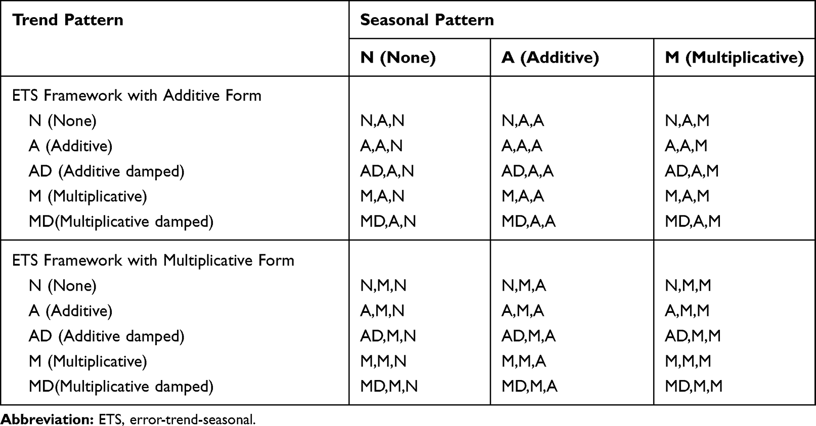Table 1 The 30 Alterative ETS Methods Associated with Various Combinations of Trend, Seasonality and Error

Performance Measures

Four measure indices including the mean absolute deviation (MAD), mean absolute percentage error (MAPE), root mean squared error (RMSE) and mean error rate (MER) were employed to compare and assess the mimic and predictive accuracies between the optimal SARIMA and ETS methods. The model that gives smaller values among the above indices in both fitting and projection parts is considered the best-performing.

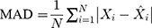
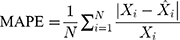
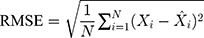
where is the actual TB incidence data, signifies the mimic and predictive TB incidence data, refers to the averages of the actual TB incidence data, represents the number of simulations and projections.

Data Analysis

We examined the secular TB epidemic trends and changes with the measures of annual percent change (APC) and average annual percentage change (AAPC) using the joinpoint regression program (version 4.7.0).²³ We employed the forecasting function of SPSS software (version 17.0, IBM Corp, Armonk, NY) and the packages of “forecast” and “tseries” of R software (version 3.4.3, R Development Core Team, Vienna, Austria) to develop the SARIMA method, and using the Eviews10.0 software (IHS, Inc. USA) to establish the ETS techniques. Statistical significance level was set at a two-sided P<0.05.

Results

Descriptive Analysis

From January 1997 until August 2019, there were 24,078,923 cases reported of TB in China with an average 88,526 cases per month, leading to an average monthly and annualized morbidity rates of 6.722 and 63.498 per 100,000 persons, respectively. As shown in Figure 1, the overall TB epidemic trend appeared to be significantly ascending with AAPC=4.167 (95% uncertainty interval: 3.104 to 5.240; Z=7.801, P<0.001) over the study period, yet since 2008, there was a clear decreasing trend in TB incidence with AAPC=−3.722 (95% uncertainty interval: −4.193 to −3.250; Z=−15.183, P<0.001). When the Seasonal-Trend decomposition procedure based on Loess (STL) was utilized to decompose the series into various components, we observed that there existed a notable cyclical fluctuation with 12 months and seasonal distribution in TB incidence, peaked in March until August of each year, particularly in March and April annually; troughed in September until February in the subsequent year, particularly in January and February annually (Figures 2 and 3).

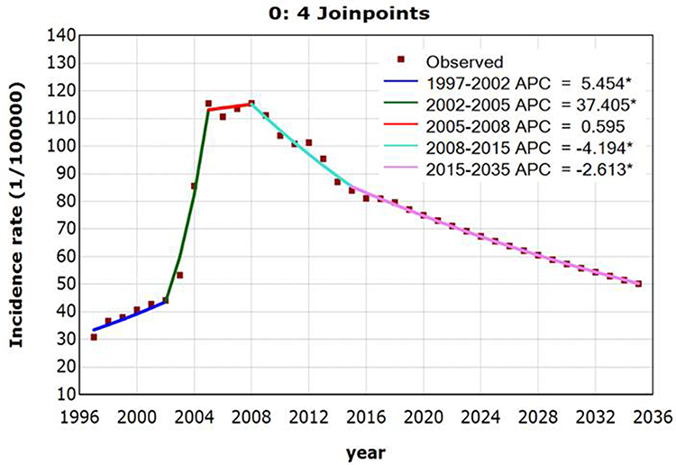Figure 1 Joinpoint regression displaying the TB epidemic trends over the period 1997–2035. *Showed that the annual percent change (APC) is significantly different from zero at the significance level.

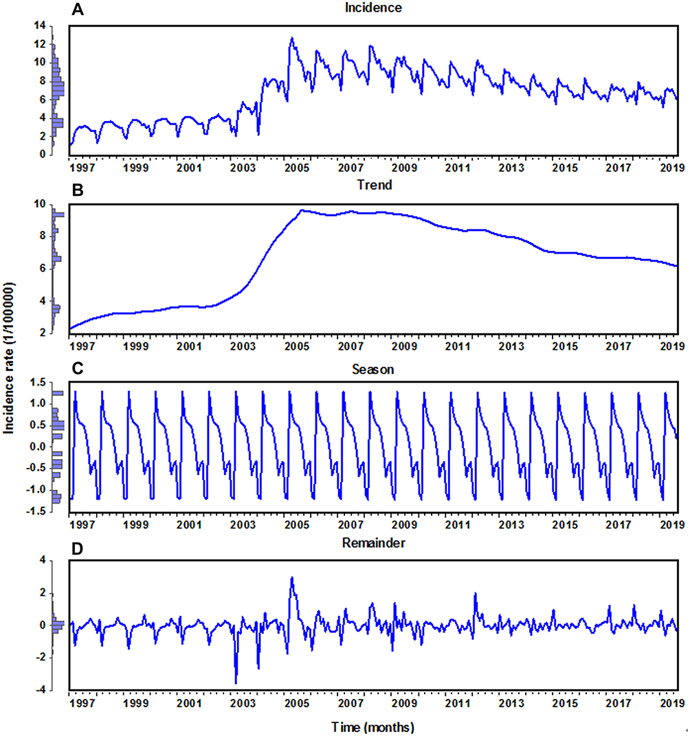Figure 2 Time-series plot for the monthly TB incidence in China from January 1997 to August 2019 and the seasonal decomposition consisting of different components of the TB series with the STL method. (A) TB incidence time series; (B) trend component; (C) seasonal component; (D) irregular component.

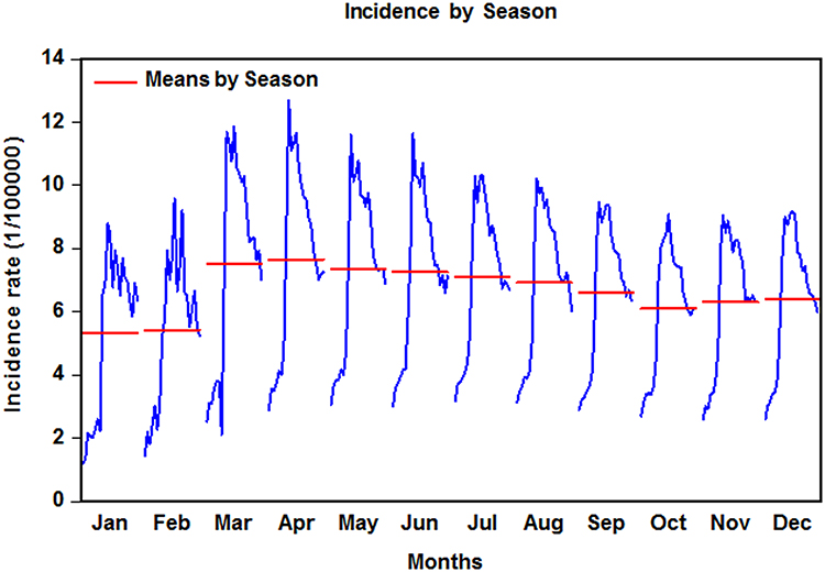Figure 3 Monthly TB incidence plot averaged by season.

The Best-Undertaking SARIMA Models

We performed an ADF test for the TB morbidity series prior to constructing models (ADF=−0.788, P=0.365), indicating that there was a unit root. Thus, based on the ADF test and the marked seasonal fluctuation in the TB incidence series (Figure 3 and S1), the log-transformation and square root transformation were applied to the series to stabilize its variance-varying over time. Looking at Figure S2, being suggestive of a similar trend between these two transformed series. We discovered that the square root transformation seemed to be more suitable for our data after trying these two approaches. Further, this transformed series was seasonally and non-seasonally differenced once, respectively, to meet the stationary need of SARIMA-developing model (ADF=−19.525, P<0.001), suggesting that it is now stationary (Figures S3 and S4). Subsequently, according to the spikes in the ACF and PACF graphs plotted with the differenced series, some possible SARIMA models were selected to perform further investigation. After attempting by trial and error, we noticed that a sparse coefficient SARIMA (0,1,(1,10))(0,1,1)₁₂ model was supposed to be the best-undertaking among all candidate models as this model gave the largest stationary R² of 0.617 and R² of 0.931 as well as the minimum normalized BIC of −0.753 (Table 2). Moreover, all the identified parameters showed a statistical significance and the residuals produced by this sparse coefficient model actualized a white noise sequence (Table 2 and Figure 4). Therefore, 12-step ahead forecasts could finally be completed by employing this best-fitting model (Figure 5A). Likewise, following the modeling procedures in the 12-data ahead predictions, we could obtain the best-performing SARIMA models for 24, 36, 48, 72, 96, 108, and 132 data ahead projections (Table 2 and Figure 5 and S5-S11).

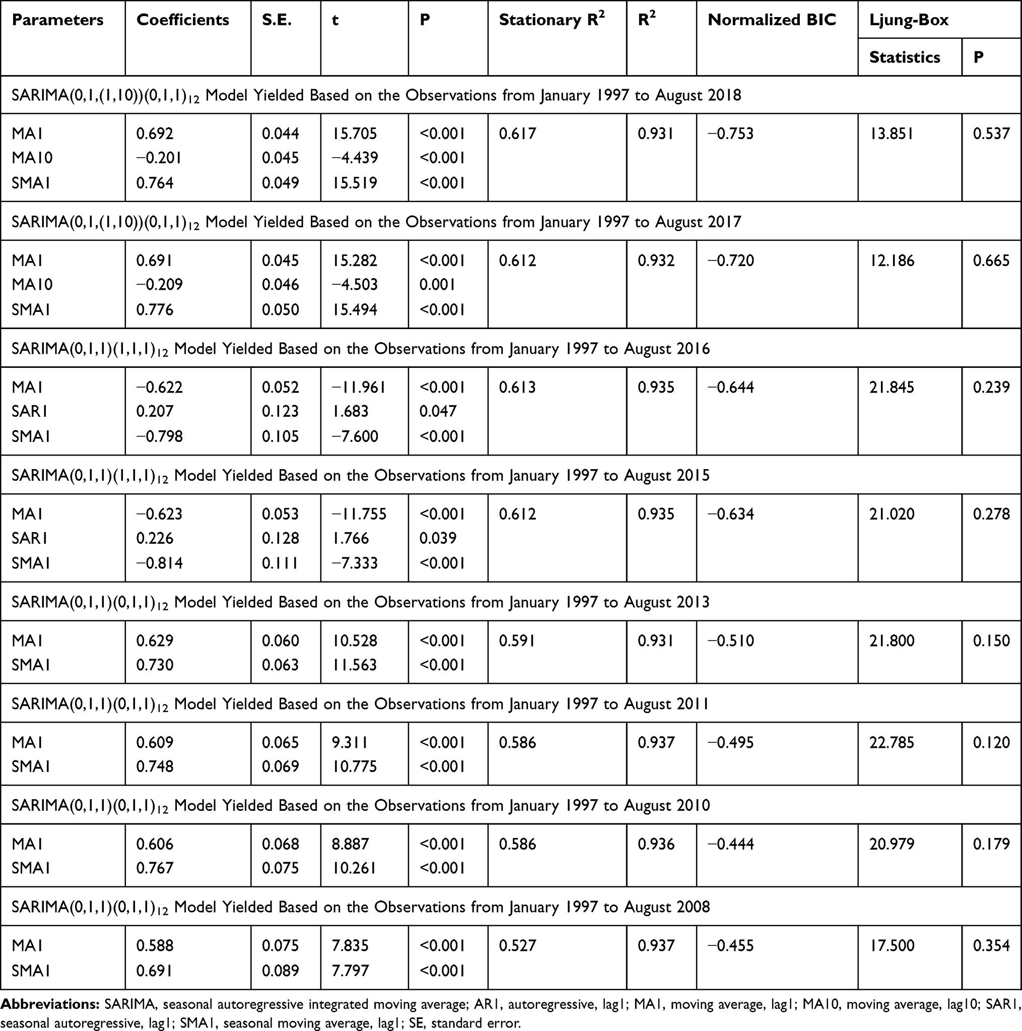Table 2 The Best-Performing SARIMA Models Obtained from Various Training Sets and Goodness of Fit Tests for Their Parameters

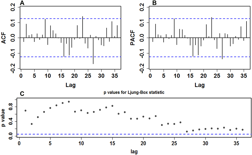Figure 4 Goodness of fit test for the residuals generated by the SARIMA(0,1,(1,10))(0,1,1)12 approach established with the training data from January 1997 to August 2018. (A) Autocorrelation function (ACF); (B) partial autocorrelation function (PACF); (C) P values for Ljung–Box statistic. Almost all of correlation coefficients fell into the 95% uncertainty levels and all P values at different lags were greater than the significance level of 0.05, indicating that this approach showed a good adequacy for this series.

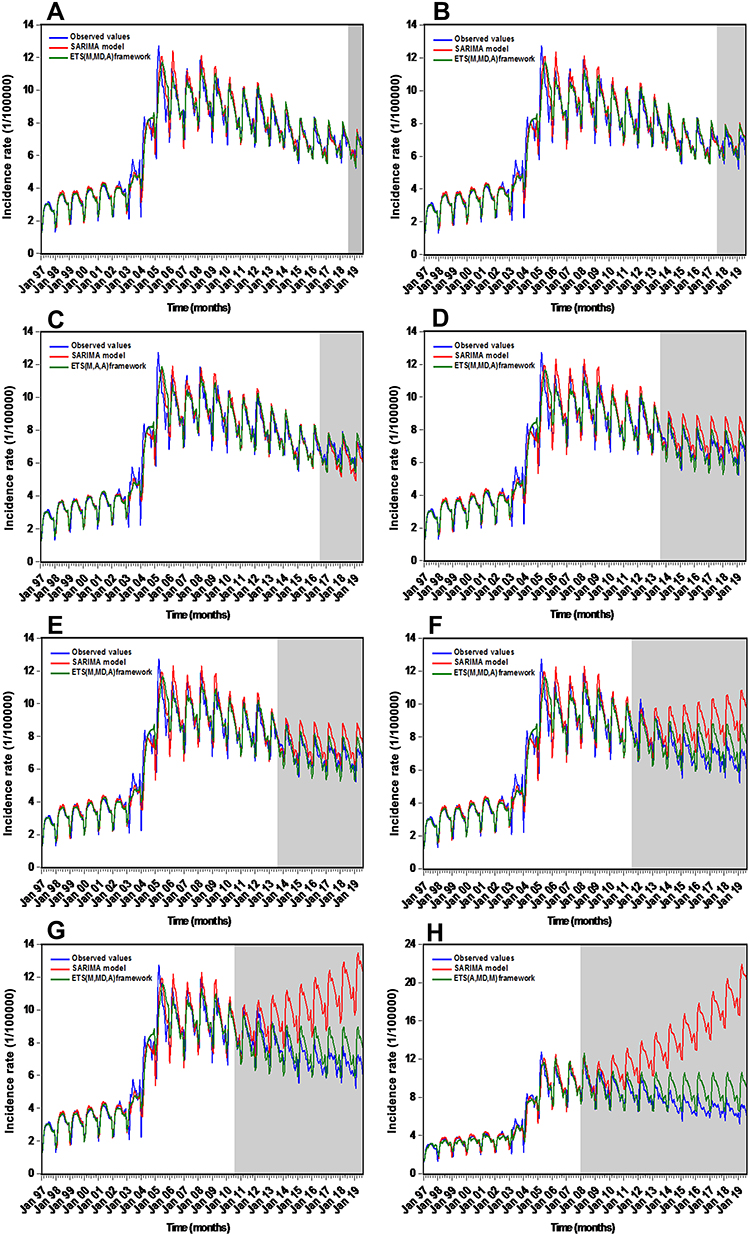Figure 5 Comparative time series plots measuring the approximations to the hold-out data on different-step-ahead predictions using the SARIMA and ETS methods. (A) 12 data ahead forecasts; (B) 24 data ahead forecasts; (C) 36 data ahead forecasts; (D) 48 data ahead forecasts; (E) 72 data ahead forecasts; (F) 96 data ahead forecasts; (G) 108 data ahead forecasts; (H) 132 data ahead forecasts. In these plots, the shaded areas displayed the predictive results using the SARIMA and ETS models, suggesting that the ETS methods captured the dependent structures well, particularly for the long-term forecasting time steps.

The Best-Undertaking ETS Models

Altogether 30 candidate models were derived by applying the ETS framework to the TB incidence data from January 1997 to August 2018 (Table S1). Among which the ETS(M,MD,A) approach composing of multiplicative errors, a damped multiplicative trend and multiplicative seasonality was expected to be elected as the best-undertaking because there were four out of six performance indices that tended to choose the ETS(M,MD,A) method (Compact LL=−590.972, LL=−237.007, AIC=1215.944, BIC=1276.475, HQ=1240.278, and AMSE=0.495), and its parameters and initial states’ values are presented in Tables 3 and S2. Furthermore, this method showed a similar performance on training and forecasting sets, so there is likely no overfitting (Table 4). Based on these results, we believed that this derived best-conducting ETS method is appropriate for the TB morbidity series forecasting (Figure 5A). In the same way, we could also identify the preferred ETS approaches used to conduct a prediction into future 24, 36, 48, 72, 96, 108 and 132 months by comparing the above six performance measures in the training subsamples and judging whether there was overfitting between training and testing subsets (Tables S3–S15 and Figure 5).

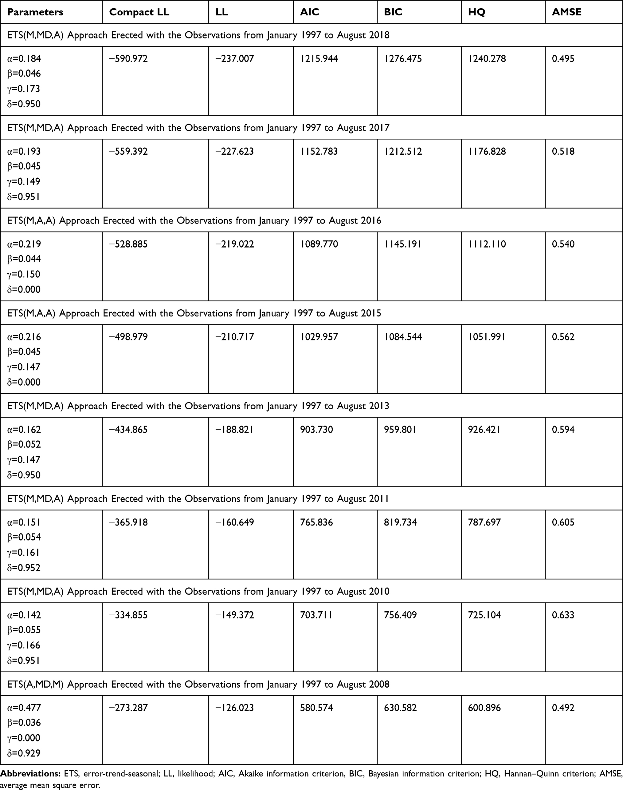Table 3 The Best-Performing ETS Models Obtained from Various Training Sets and Goodness of Fit Tests for Their Parameters

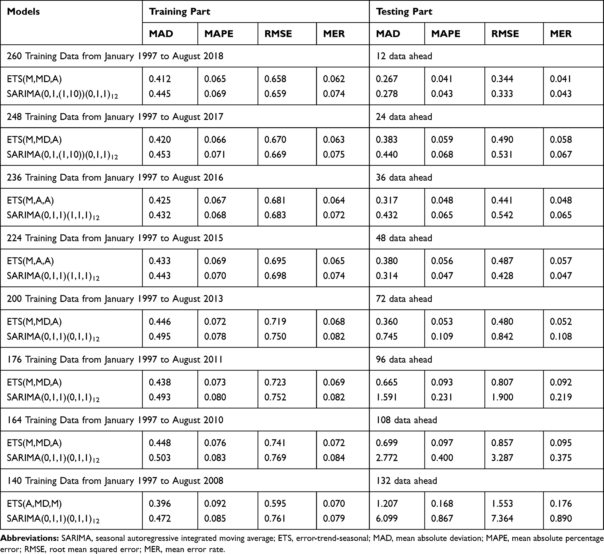Table 4 Comparative Results of the Performances Between the Best-Undertaking SARIMA Methods and the Best-Undertaking ETS Methods on the Different Training and Testing Sets

Performance Comparisons Among Models

The constructed ETS methods were compared with the SARIMA approaches from two aspects of simulation and projection based on the measures including MAD, MAPE, RMSE, and MER. As shown in Table 4, it was seen that the ETS models displayed lower values of performance indices in both training and testing sets except for the 48-step ahead forecasting. And as presented in Figure 5, together the ETS approaches could better capture the secular epidemic trends and seasonality of TB incidence though the predictive accuracies continued to slightly degrade, in tandem with the increases of the ahead forecasting time steps. By contrast, the SARIMA models have deviated from the epidemic trajectories of TB morbidity after 48-data ahead forecasting. Due to its superiority of the ETS framework in modeling TB morbidity series, we thus established the ETS(M,M,M) method derived from the entire dataset to project TB incidence rate into 2035 (Figure 6). As illustrated in Figure 1, albeit the TB incidence continued to display a downward trend at 2.613% (95% uncertainty interval: 2.473% to 2.752%) per year during the projection periods, it showed major challenges ahead to achieve the WHO’s milestones and goals in China.

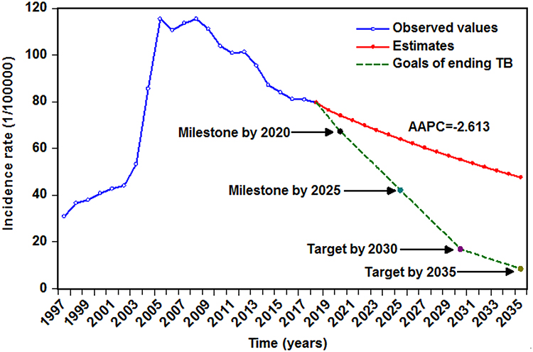Figure 6 Annual TB incidence projections up to 2035 using the ETS(M,M,M) method based on the entire dataset. As illustrated, albeit the TB incidence continued to display a declined trend at 2.613% per year in China, it showed major challenges ahead to achieve the WHO’s milestones and goals.

Discussion

TB invariably remains a major public health issue in China and worldwide.¹ Early warning for its long-term epidemic trajectories may serve as a base for the decision-making process and facilitate the allocation of health-care resource under dynamic demand. In this work, we explored its potential of the ETS framework and its suitability through a series of comparative experiments for the application in analyzing and estimating the long-term epidemic seasonality and trends of TB incidence in China. As far as we know, no published research has been found until now to perform a long-run TB incidence prediction using this framework. Our findings revealed that by comparison with the SARIMA models, overall the ETS techniques provide a higher-precision approximation to the secular seasonality and trends of TB incidence in both the short-run and long-run forecasting periods. Moreover, although there is a reduction performance with the increased time steps, the long-term predictive results still remain robust and reliable as the performance measure of MAPE presents a value of less than 0.2 in all multi-step-ahead predictions. The MAPE value is commonly utilized to measure accuracy of a forecast, a model with this index value lower than 0.2 is deemed good.¹³ Our prior study documented that the mixed SARIMA-nonlinear autoregressive neural network with exogenous variables technique also has the potential to assess the secular epidemic trends of TB notified cases, in which the prediction performance into the future 75 time steps was MAPE=0.221.²⁴ However, we found that the ETS framework (MAPE=0.053 and MAPE=0.093 for 72-data and 96-data ahead forecasting, respectively) still showed a remarkable improvement over the above mixed method by comparing their forecasting performances. Therefore, the ETS models can emerge as a useful tool in studying the long-term epidemic patterns of TB incidence in China. Further, this ETS framework can also play an important part in evaluating the long-term effects of new prophylaxis, such as the optimization of the current tools, the introduction of the new vaccine, the directly observed antimicrobial treatment, and/or other intervention strategies. If the estimated TB epidemic levels are higher than that of the actual after a new intervention has been applied in the population, showing that such a measure is effective. Besides, we noted that the predictive results using the SARIMA model were highly accurate before 48-data ahead, whereas after that, this model failed to be applicable to estimate the TB epidemic behaviors. This finding further validates the usefulness of ARIMA as a short-or medium-term forecasting method.

The ARIMA method is comprised of an autoregressive method and a moving average method.²⁵ Since this approach is without requirement for a previous assumption regarding the development model of a time series; hence, it has widely been adopted to model diseases morbidity or mortality time series with both non-seasonality and seasonality.²⁶ Even for a non-stationary time series, after preprocessing with the transformed method of logarithm or square root and/or difference, the ARIMA model is also applicable.²⁵ For instance, Liu et al established a SARIMA(0,1,2)(0,1,1)₁₂ method to estimate the TB epidemic trends in Jiangsu Province of China.²⁶ Earnest et al constructed an ARIMA (1,1,0) approach to forecast the prostate cancer incidence and mortality rates in Australia.²⁷ Though the above models attained a satisfactory performance for their target time series, the linear essence of the ARIMA model gives rise to a restricted capability to unearth the non-linear relationship in a time series,¹⁸ this may account for the reason that the ARIMA model is adept in conducting short-  or medium-term predictions. Nevertheless, differing from the ARIMA model, for a given either stationary or non-stationary time series, the ETS framework containing 30 possible combinations of error, trend, and seasonality by incorporating the conventional ES techniques with the state space techniques can not only explore the linear relationship using its seasonality and trend terms but investigate the non-linear relationship with its error term,¹⁵ which enables it to extract both linear and nonlinear information. Considering its superiority of the ETS framework in analyzing time series, it appears that this framework may be transferable to investigate the long-term epidemic patterns for other infectious diseases or TB incidence in other areas, while much work is still needed to validate its suitability. In addition, it should be noted that the Lee-Carter and GenericPred methods are recently shown to be helpful in examining the long-term epidemic behaviors of diseases incidence.^11,28 Thus, future researches are expected to make comparison about their long-term forecasting performances between the ETS framework and the above-mentioned methods. Another worth noting is that there may be underprojection or overprojection during the process of ETS model development, which may have an effect on its generalization ability of this model.²⁶ In our research, to avoid such an effect, we selected the preferred ETS model based on multiple performance indices, and then we could identify whether there was an underfitting or overfitting by comparing their performances between in-sample data and hold-out data. As such, we can eventually obtain the optimal and the most appropriate one.

In this study, we detected that TB is a seasonal disease with high-risk seasons mainly occurring in spring and early summer. The seasonal characteristics agree with those observed in earlier researches in China,^24,29 also in line with those in the United States, Korea, Mongolia, and Kuwait.³⁰ But inconsistent with whose in Spain (which peaked June),³¹ Japan (which showed a semi-annual high-risk season peaking in June and October, respectively),³² and Iraq (which peaked in spring and winter).³³ To date, there is in the absence of exact causes that can be used to account for the seasonal patterns of TB incidence in China, yet given that there is an average incubation period of 4 to 8 weeks from TB infection to onset of symptoms and it still is required for an about 2-month delay from symptom appearance to clinical diagnosis.³⁴ The following causes seem to be of special concern. Firstly, growing work has been documenting that ambient air pollutants including PM_2.5, PM₁₀, CO, NO₂, O₃, SO₂ and air quality index (AQI) are positively linked with TB seasonality.^35,36 While the air pollutant has been a major public health problem in recent years in China, especially in winter per year, the mean concentrations of pollutants are much higher than their standards.³⁵ Secondly, a previous systematic review and meta-analysis suggested a positive correlation between low serum vitamin D levels and TB.³⁷ Importantly, several studies have found that the decreased sunshine hours and its potential effect on vitamin D levels in winter appear to be in relation to TB incidence.^38,39 Nonetheless, further studies with strong causal inference are required to verify this potential mechanism. Thirdly, greater indoor crowding in winter may lead to an increased likelihood of TB transmission.³² Finally, the most important reasons may be attributed to the “spring festival effect”, prior publications have provided an in-depth discussion regarding this effect.²⁹ Additionally, the hunt for other plausible interpretations for the seasonal distribution of TB incidence is supposed to go on.

TB incidence has continued to be plunging at the rate of 3.722% annually in China since 2008, which may be closely related to the government’s ongoing efforts such as the increased scale up of vaccination coverage, the increasingly improved monitoring system for infectious diseases, an increased budget and an effective control and treatment.²⁵ Nevertheless, the downturn of TB morbidity starts to retard to be falling at 2.613% per year since 2015, which may be ascribed to the continuously upsurged drug-resistant TB, the increased floating population and the coinfections of HIV-TB as well as other TB-related comorbidities such as influenza, diabetes and hypertension, and the like in recent years.^1,7,8 Further, we used the ETS framework to estimate the TB incidence into future until 2035, indicating that TB incidence rate will continue to descend at about 2.613% per year between 2019 and 2035. But such a rate of decline in TB incidence being reached falls far short of what is required to achieve the WHO’s milestones for 2020 and 2025 and targets for 2030 and 2035.² Therefore, there is still an urgent need for China that takes particular measures to dramatically accelerate the progress toward eliminating TB.

The occurrence of TB is often affected and constrained by many complicated factors, which enables the TB incidence series to exhibit complex linear and nonlinear interactions, and thus simply using the single linear or non-linear methods fails to excavate its entire information reasonably well.^29,40 In this study, we devoted to constructing a forecasting method with robust and accurate performance that can be used to analyze and estimate its secular trends and seasonal variation by considering the linear and non-linear clues hidden behind the TB morbidity series in China simultaneously. Moreover, the results emerged from a series of comparative experiments proved that we have succeeded. Nevertheless, there are still some shortcomings. Firstly, the TB incidence data used in our analysis are derived from the passive monitoring system of notifiable infectious diseases, the underreporting is thus inevitable. Secondly, we cannot obtain the detailed information (age and sex) concerning the TB cases, which precludes further sensitivity analysis in our work. Finally, the current findings might not be representative of the ETS framework is applicable for long-term forecasting for other infectious diseases, further experiments are still required.

Conclusions

The ETS framework can be used to undertake long-term forecasting for the epidemic trends and seasonality of TB incidence, and thus helping health professionals and decision-makers in offering advanced warning for epidemic characteristics of TB in order to better inform prevention initiatives depending on the early detection for its long-term trends. Besides, under the present dropping trend of TB incidence, it is unlikely to realize the goals of ending TB epidemic by 2035. It is imperative that a particular TB control programme should be formulated to address this issue.

References

1. Singh R, Dwivedi SP, Gaharwar US, Meena R, Rajamani P, Prasad T. Recent updates on drug resistance in Mycobacterium tuberculosis. J Appl Microbiol. 2019;1–21. doi:10.1111/jam.14478
2. WHO. Global tuberculosis report. 2019. Available from: https://wwwwhoint/tb/publications/global_report/en/.
3. WHO. Global strategy and targets for tuberculosis prevention, care and control after 2015. Available from: https://wwwwhoint/tb/post2015_strategy/en/.
4. Zhou C, Long Q, Chen J, et al. Factors that determine catastrophic expenditure for tuberculosis care: a patient survey in China. Infect Dis Poverty. 2016;5:6. doi:10.1186/s40249-016-0100-6
5. Xu CH, Jeyashree K, Shewade HD, et al. Inequity in catastrophic costs among tuberculosis-affected households in China. Infect Dis Poverty. 2019;8(1):46. doi:10.1186/s40249-019-0564-2
6. WHO. The End TB Strategy. 2014. Available from: https://wwwwhoint/tb/End_TB_brochurepdf.
7. Ayelign B, Negash M. Immunological impacts of diabetes on the susceptibility of mycobacterium tuberculosis. J Immunol Res. 2019;2019:6196532. doi:10.1155/2019/6196532
8. Walaza S, Cohen C, Tempia S, et al. Influenza and tuberculosis co-infection: a systematic review. Influenza Other Respir Viruses. 2019. doi:10.1111/irv.12670
9. Zhou Q, Jiang H, Wang J, Zhou J. A hybrid model for PM2.5 forecasting based on ensemble empirical mode decomposition and a general regression neural network. Sci Total Environ. 2014;496:264–274. doi:10.1016/j.scitotenv.2014.07.051
10. Khan MT, Kaushik AC, Ji L, Malik SI, Ali S, Wei DQ. Artificial neural networks for prediction of tuberculosis disease. Front Microbiol. 2019;10:395. doi:10.3389/fmicb.2019.00395
11. Golestani A, Gras R. Can we predict the unpredictable? Sci Rep. 2014;4:6834. doi:10.1038/srep06834
12. Chatfield C, Koehler AB, Ord JK, Snyder RD. A new look at models for exponential smoothing. J R Stat Soc. 2001;50(2):147–159. doi:10.1111/1467-9884.00267
13. Ke G, Hu Y, Huang X, et al. Epidemiological analysis of hemorrhagic fever with renal syndrome in China with the seasonal-trend decomposition method and the exponential smoothing model. Sci Rep. 2016;6:39350. doi:10.1038/srep39350
14. Hyndman RJ, Khandakar Y. Automatic time series forecasting: the forecast package for R. J Stat Softw. 2008;27(3):1–22. doi:10.18637/jss.v027.i03
15. Hyndman RJ, Koehler AB, Keith OJ, Snyder RD. Forecasting with Exponential Smoothing the State Space Approach. berlin: springer-verlag; 2008.
16. Zhang X, Pang Y, Cui M, Stallones L, Xiang H. Forecasting mortality of road traffic injuries in China using seasonal autoregressive integrated moving average model. Ann Epidemiol. 2015;25(2):101–106. doi:10.1016/j.annepidem.2014.10.015
17. Mao Q, Zhang K, Yan W, Cheng C. Forecasting the incidence of tuberculosis in China using the seasonal auto-regressive integrated moving average (SARIMA) model. J Infect Public Health. 2018;11(5):707–712. doi:10.1016/j.jiph.2018.04.009
18. Wei W, Jiang J, Liang H, et al. Application of a combined model with Autoregressive Integrated Moving Average (ARIMA) and Generalized Regression Neural Network (GRNN) in forecasting hepatitis incidence in Heng County, China. PLoS One. 2016;11(6):e0156768. doi:10.1371/journal.pone.0156768
19. Wang YW, Shen ZZ, Jiang Y. Comparison of autoregressive integrated moving average model and generalised regression neural network model for prediction of haemorrhagic fever with renal syndrome in China: a time-series study. BMJ Open. 2019;9(6):e025773. doi:10.1136/bmjopen-2018-025773
20. Wu W, An SY, Guan P, Huang DS, Zhou BS. Time series analysis of human brucellosis in mainland China by using Elman and Jordan recurrent neural networks. BMC Infect Dis. 2019;19(1):414. doi:10.1186/s12879-019-4028-x
21. Hyndman RJ, Koehler AB, Snyder RD, Grose S. A state space framework for automatic forecasting using exponential smoothing methods. Int J Forecast. 2000;18(3):439–454. doi:10.1016/S0169-2070(01)00110-8
22. Wang Y, Xu C, Zhang S, Wang Z, Zhu Y, Yuan J. Temporal trends analysis of human brucellosis incidence in mainland China from 2004 to 2018. Sci Rep. 2018;8(1):15901. doi:10.1038/s41598-018-33165-9
23. Zhao Y, Lafta R, Hagopian A, Flaxman AD. The epidemiology of 32 selected communicable diseases in Iraq, 2004-2016. Int J Infect Dis. 2019;89:102–109. doi:10.1016/j.ijid.2019.09.018
24. Wang Y, Xu C, Zhang S, et al. Temporal trends analysis of tuberculosis morbidity in mainland China from 1997 to 2025 using a new SARIMA-NARNNX hybrid model. BMJ Open. 2019;9(7):e024409. doi:10.1136/bmjopen-2018-024409
25. Li Z, Wang Z, Song H, et al. Application of a hybrid model in predicting the incidence of tuberculosis in a Chinese population. Infect Drug Resist. 2019;12:1011–1020. doi:10.2147/idr.s190418
26. Liu Q, Li Z, Ji Y, et al. Forecasting the seasonality and trend of pulmonary tuberculosis in Jiangsu Province of China using advanced statistical time-series analyses. Infect Drug Resist. 2019;12:2311–2322. doi:10.2147/idr.s207809
27. Earnest A, Evans SM, Sampurno F, Millar J. Forecasting annual incidence and mortality rate for prostate cancer in Australia until 2022 using autoregressive integrated moving average (ARIMA) models. BMJ Open. 2019;9(8):e031331. doi:10.1136/bmjopen-2019-031331
28. Ku CC, Dodd PJ. Forecasting the impact of population ageing on tuberculosis incidence. PLoS One. 2019;14(9):e0222937. doi:10.1371/journal.pone.0222937
29. Cao S, Wang F, Tam W, et al. A hybrid seasonal prediction model for tuberculosis incidence in China. BMC Med Inform Decis Mak. 2013;13(1):56. doi:10.1186/1472-6947-13-56
30. Kim EH, Bae JM. Seasonality of tuberculosis in the Republic of Korea, 2006-2016. Epi Heal. 2018;40:e2018051. doi:10.4178/epih.e2018051
31. Luquero FJ, Sanchez-padilla E, Simon-soria F, Eiros JM, Golub JE. Trend and seasonality of tuberculosis in Spain, 1996-2004. Int J Tuberc Lung Dis. 2008;12(2):221–224.
32. Sumi A, Kobayashi N. Time-series analysis of geographically specific monthly number of newly registered cases of active tuberculosis in Japan. PLoS One. 2019;14(3):e0213856. doi:10.1371/journal.pone.0213856
33. Mohammed SH, Ahmed MM, Al-mousawi AM, Azeez A. Seasonal behavior and forecasting trends of tuberculosis incidence in Holy Kerbala, Iraq. Int J Mycobacteriol. 2018;7(4):361–367. doi:10.4103/ijmy.ijmy_109_18
34. Li XX, Wang LX, Zhang H, et al. Seasonal variations in notification of active tuberculosis cases in China, 2005-2012. PLoS One. 2013;8(7):e68102. doi:10.1371/journal.pone.0068102
35. Wang H, Tian C, Wang W, Luo X. Temporal cross-correlations between ambient air pollutants and seasonality of tuberculosis: a time-series analysis. Int J Environ Res Public Health. 2019;16(9). doi:10.3390/ijerph16091585
36. Blount RJ, Pascopella L, Catanzaro DG, et al. Traffic-related air pollution and all-cause mortality during tuberculosis treatment in California. Environ Health Perspect. 2017;125(9):097026. doi:10.1289/ehp1699
37. Nnoaham KE, Clarke A. Low serum vitamin D levels and tuberculosis: a systematic review and meta-analysis. Int J Epidemiol. 2008;37(1):113–119. doi:10.1093/ije/dym247
38. Xiao Y, He L, Chen Y, et al. The influence of meteorological factors on tuberculosis incidence in Southwest China from 2006 to 2015. Sci Rep. 2018;8(1):10053. doi:10.1038/s41598-018-28426-6
39. Koh GC, Hawthorne G, Turner AM, Kunst H, Dedicoat M. Tuberculosis incidence correlates with sunshine: an ecological 28-year time series study. PLoS One. 2013;8(3):e57752. doi:10.1371/journal.pone.0057752
40. Xu G, Mao X, Wang J, Pan H. Clustering and recent transmission of Mycobacterium tuberculosis in a Chinese population. Infect Drug Resist. 2018;11:323–330. doi:10.2147/idr.s156534
© 2020 The Author(s). This work is published and licensed by Dove Medical Press Limited. The full terms of this license are available at https://www.dovepress.com/terms.php and incorporate the Creative Commons Attribution - Non Commercial (unported, v3.0) License.
By accessing the work you hereby accept the Terms. Non-commercial uses of the work are permitted without any further permission from Dove Medical Press Limited, provided the work is properly attributed. For permission for commercial use of this work, please see paragraphs 4.2 and 5 of our Terms.