Reconstructing brain magnetic susceptibility distributions from T2* phase images by TV-regularized 2-subproblem split Bregman iterations

Introduction

It is known that the source of T2*-weighted magnetic resonance imaging (T2*MRI) involves a diversity of causes,¹ including fieldmap inhomogeneity (T2′ effect), random spin–spin interaction (tissue-specific T2 effect), as well as random spin diffusion. Through the use of an EPI (echo-planar imaging) sequence, a T2*MRI study produces an output of complex-valued image (denoted by T2* complex image) consisting of a pair of magnitude and phase components (denoted by T2* magnitude image and T2* phase image). For brain imaging, the underlying source of T2*MRI is primarily an inhomogeneous magnetic susceptibility distribution (denoted by χ) of brain tissues, which undergoes a magnetization process (or magnetic polarization) in a main field and incurs an inhomogeneous fieldmap for T2*-effect image formation. The intra-cranial dynamic χ perturbation associated with a neuronal activity has been described by the BOLD fMRI model (blood oxygenation level dependent functional MRI).^2–4 In principle, for brain imaging, we can reconstruct the χ-expressed source from T2* complex images by solving an inverse problem (a 3D deconvolution problem), which provides a more direct representation of the brain state (either a static anatomic or a dynamic functional state) than the T2*MRI-acquired image (experimental raw data), primarily due to the removal of dipole effect. This consensus has inspired discussion of the hot topic of quantitative susceptibility mapping (QSM),^5–12 which is also termed magnetic susceptibility tomography (denoted by χ tomography) in the context of medical imaging,^13–15 conveying the digital internal source reproduction from observed images with spatial conformance by computationally solving an inverse problem.

A T2*MRI procedure involves a 3D spatial convolution that describes a fieldmap formation as a result of material magnetization in a main field.^7,13,16 Due to the spatial spread and anisotropy of the 3D convolution kernel (dipole field distribution), the 3D magnetization process dictates a morphological mismatch between the input source χ (intrinsic magnetic property of material) and either the magnitude or phase of the output T2* complex image. Recent research^{7,12,13,17,18} has shown that the χ tomography can be implemented by performing an inverse T2*MRI computation, as described by computed inverse MRI (CIMRI).¹³ The core technology of CIMRI-based χ tomography lies in solving the inverse problem of the 3D convolution, an ill-posed 3D deconvolution problem.

In principle, 3D magnetic susceptibility reconstruction from a fieldmap could be completely solved via matrix algebra,^17,19,20 which involves converting the 3D convolution operation into a matrix equation (with a 2D convolutional matrix) and performing a Tikhonov regularization on the ill-conditioned matrix. In practice, this matrix inverse method is limited to a small χ map reconstruction (typically less than 16 × 16 × 16),¹⁷ due to the computational difficulty of finding the inverse of a large matrix.

In the Fourier domain, a 3D deconvolution is represented by a 3D inverse filtering that involves 3D element-wise division. Due to a zero surface embedded in the 3D convolution kernel, the inverse filtering suffers from a divide-by-zero problem. The simplest way to regularize the divide-by-zero singularity is to truncate the inverse filter at the zero surface by thresholding (called filter truncation), which has been used for reconstructing brain χ maps.^6,8,10,12,21 However, the data alteration due to truncation regularization may cause stripe artifacts^6,10,12 and non-conservation of image energy (image intensity values).¹³

Recently, total variation (TV) regularization has been explored for iterative image restoration.^22–25 It has been shown that a TV-regularized minimization problem can be effectively implemented by a split Bregman iteration technique.^22,23 In the framework of numerical methods and convex optimization theory, the split Bregman TV iteration method is excellent for image restoration in the presence of noise, blurring, and in-painting contaminations. More details about the 2D TV-regularized image restoration theory can be found in various studies.^{22,23,26–28} We have generalized the 2D TV-regularized image restoration method for 3D χ tomography with a 3-subproblem split scheme.¹³ In this paper, we will report on a 3D TV-regularized iteration with a 2-subproblem Bregman split algorithm, which can efficiently provide an intact brain magnetic susceptibility state from T2* phase image.

Methods

Feldmap establishment in T2*MRI

Let χ(x, y, z) denote the χ expression (intrinsic magnetic property) of an object under scanning, and b(x, y, z) the fieldmap (specifically, the z-component of the vector field resulting from material magnetization in a main field B₀). Under linear magnetization of non-magnetic (strictly weak-magnetic) material such as brain tissues for brain imaging, the χ-induced fieldmap is related to the susceptibility distribution by a 3D convolution by^16,29

where * denotes a 3D convolution, r = (x, y, z) the space domain, h(r) is a convolution kernel (the field distribution of a point magnetic dipole),³⁰ and ε(r) the additive noise. By configuring the random vascular geometry in a brain cortical region, we can simulate χ-expressed brain physiological state. Under vascular blood magnetization in a B₀ field, we can calculate the χ-induced fieldmap by Equation 1, thereby numerically simulating the multivoxel brain functional imaging.^13,31,32 According to h(r) ≠ δ(r), b(r) is morphologically different from χ(r) by a 3D spatial convolution in Equation 1, which is described as the dipole effect.

Implementation of χ tomography: CIMRI

Let C(x, y, z) denote a T2* complex image acquired by T2*MRI with an echo time T_E, its magnitude image is defined by A₀(x, y, z) = |C(x, y, z)|, and its phase by P₀(x, y, z) = ∠C(x, y, z). For magnitude images, we are concerned with the magnitude loss which assumes minimal zeros in the non-decay regions and maximal numbers in the most decay regions. For convenience, we normalize the magnitude image to [0,1], whereas the phase image is normalized to the range (−π, π] radian. For an n-bit digital phase data, we convert the digital number into a radian expressed by

For numerical simulations, we can directly calculate the magnitude loss images and phase angle accrual images from T2* complex images.³³

In a small phase angle regime (a linear phase approximation condition: exp(iφ) ≈ 1 + iφ), the fieldmap is related to the phase image by³⁴

where ‘s.t.’ stands for ‘subject to’. It is observed that the phase angle accrual is linearly proportional to T_E and b(x, y, z) in Equation 3, and the main field B₀ plays a scale factor in the fieldmap establishment in Equation 1. The linear scale relation in Equation 3 indicates no information loss between the fieldmap and the T2* phase image, which allows us to calculate the susceptibility source (denoted by χ^recon(x, y, z)) from the fieldmap by solving the inverse problem of Equation 1, that is,

where *⁻¹ denotes deconvolution, and h(x, y, z) the same kernel as used for the 3D convolution defined in Equation 1. The main topic in this report focuses on technically solving the 3D deconvolution problem in Equation 4, or conceptually implementing dipole inversion.

The small phase angle regime in Equation 3 is a strict condition of theoretical linear approximation of intravoxel dephasing signal (subject to |P|<<π). In practice, the fieldmap is usually calculated from a phase image (unwrapping is needed when phase angle is wrapped, |P|>π).⁶ For brain imaging experiments with 30 milliseconds T_E, the phase angle of complex EPI data is usually small (typically <0.3 rad) such that it remains phase unwrapped in the brain cortex region. Approximately, we can calculate the intracranial fieldmap from the brain T2* phase image using Equation 3, and thereby proceed to reconstruct the intracranial χ distribution using Equation 4.

Deconvolution solvers

In general, the 3D deconvolution solvers can be classified into three categories:¹³ Tikhonov-regularized matrix inverse, inverse filtering by truncating the singular inverse filter, and iteration minimization. It has been shown that the matrix inverse solver is limited to applications to small 3D multivoxel images,¹⁷ and that both the 3D inverse filtering and 3D TV iteration solvers manipulate the 3D matrices in a manner of element-wise arithmetic (addition, subtraction, multiplication, and division), which allows us to accommodate a large 3D matrix effortlessly (eg, 512 × 512 × 512). In what follows, we will only address the filter truncation and TV iteration solvers.

Inverse filtering (filter truncation solver)

In the Fourier domain, the 3D convolution in Equation 1 is converted into a 3D multiplication formula. The inverse filtering with truncated inverse filter can be expressed by^{6,13,33,35,36}

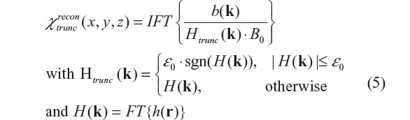
where FT and IFT stand for Fourier transform and inverse Fourier transform, respectively, b(k) denotes the Fourier transform of b(r), sgn a sign function (sgn(t) =1 for t≥0 and =–1 for t<0), and ε₀ a small constant for truncation threshold.^6,13 The implementation of filter truncation in Equation 5 may assume a variation, such as using a distributive threshold map rather than a constant⁶ and ignoring the sign.¹² Due to data alteration resulting from thresholding, the χ reconstruction by using Equation 5 suffers from stripe artifacts^10,11 and image energy non-conservation.³³

TV-regularized split Bregman iteration (TV iteration solver)

In this subsection, we generalize the TV-regularized iteration algorithm to accommodate our 3D deconvolution problem that has a 3D anisotropic bipolar-valued convolution kernel.¹³

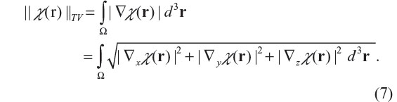
Mathematically, the TV norm for 3D χ(r) is defined as

where g denotes a vector functional variable that is bounded by |g|≤1, and Ω the 3D space domain over which χ(r) is defined, ▽ the spatial gradient operator, and ||·||₈ the infinite norm (maximum norm). Strictly speaking, ||χ||_TV is a semi-norm in which ||χ||_TV =0 is allowed for χ≠0. For a 3D smooth function χ(r), the TV norm is also given by³⁷

For a non-differentiable function χ(r), the gradient is interpreted as subgradient (a subgradient of J at v, denoted by ∂J(v), is defined by an inequality: J(u) – J(v) ≥ <∂J(v), u– v> for all u around v, where <x, y> denotes the inner product between x and y). Assuming a Gaussian noise model for ε(r), we can solve the inverse problem (as expressed in Equation 4) by a TV-regularized unconstrained minimization problem,^{22,23,26–28} as expressed by

where BV is a bounded variation function space, and λ is the Lagrange multiplier or the regularization parameter. The TV regularization lies in its searching over all possible distributions in a bounded variation space (χ∈BV) to find an optimal distribution χ^recon such that it minimizes TV norm and the data fidelity error simultaneously. The algorithm implementation of Equation 8 is nontrivial. Recent research^13,22,38 has shown that the TV iteration can be effectively implemented by a split Bregman iteration algorithm. The basic idea of the split Bregman algorithm is to transform a constrained optimization problem into a series of unconstrained subproblems, and then to solve each subproblem by a Bregman-distance-based iteration. The Bregman distance is defined for an objective function J(u) as

where ∂J(v) is a subgradient of function J(v) at v. The subgradient ∂J(v) is used to relax the differentiation condition so as to admit spatial discontinuity (jumps) and non-smoothness. For a spatial differentiable distribution, a subgradient reduces to a regular gradient. Intuitively, the Bregman distance in Equation 9 can be construed to be the difference between the value of function J at point u and the value of the first-order Taylor expansion of J around point v evaluated at point u. It has been proved that the use of Bregman distance in Equation 9 can ensure fast convergence.^22,23

Let J(χ)=||χ||_TV with an initialization of χ₀ =0, then the Bregman iteration produces a series {χ_k, k =1, 2, …} by

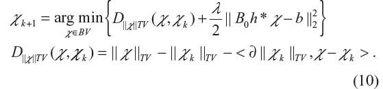
The Bregman iteration can also be equivalently achieved by introducing an auxiliary variable u and carrying out the following iteration (with initiation u₀ =0)

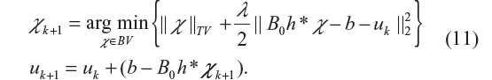
In the result, the Bregman iteration produces a series {(χ_k, u_k), k =1, 2, …}. It is noted that u_k is updated by adding back the residual in Equation 11, which may manifest as comeback noise (usually appearing randomly and sparsely in uniform regions). The iteration is stopped when a criterion is satisfied or the specified maximum iteration number is reached.

To solve our 3D deconvolution problem in Equation 8, we need to cope with the Bregman iterations in Equation 10 or Equation 11 in 3D scenarios. In our previous publication,¹³ we report on a 3-subproblem split Bregman iteration algorithm, which splits the TV-regularized minimization problem into three Bregman iteration subproblems. We refer readers to other studies^22,23 for mathematical details. In what follows, we propose a 2-subproblem split Bregman iteration algorithm for 3D χ reconstruction with easy implementation. By introducing an auxiliary variable d=▽χ, we can convert the 3D deconvolution in Equation 8 into a minimization problem of two split Bregman TV iteration subproblems, that is

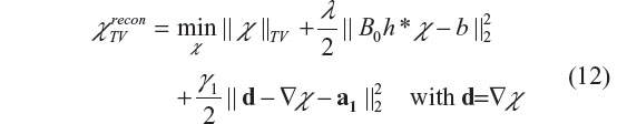
where the parameters {γ₁, a₁} are introduced for splitting the regularization term (the data fidelity term in Equation 8) and for fast convergence. In particular, γ₁ is a built-in regularization parameter in an iteration program, that can be set to a constant, for example, γ₁ =5 as suggested by Goldstein and Osher,²³ and Chambolle and Lions;²⁶ a₁ is an iterative vector variable, that is updated during each iteration. The split two subproblems (with respect to {‘d’,‘χ’}) are alternatively iterated, solving one subproblem at a time while keeping the other fixed. There exist closed forms for the 2-subproblem Bregman iterations which can be described as follows.

1. The d-subproblem, with χ fixed, is



Its solution in a closed form is given by^22,23



2. The χ-subproblem, with d fixed, is

In the Fourier domain, the optimization equation of the minimization problem in Equation 15 is given by^22,23

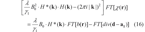
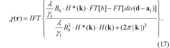
where ‘div’ denotes vector divergence, and FT stands for Fourier transform. Therefore, the solution of the χ-subproblem minimization is given by

In programming implementation, the 2-subproblem split Bregman iteration algorithm for the TV-regularized minimization problem in Equation 12 can be summarized by the following algorithm^22,23

Initialize χ=0, d=a₁=0

Do

Minimization of χ-subproblem with d fixed;

Minimization of d-subproblem with χ fixed;

Update a₁: =a₁+▽χ–d

While ‘not converged’

The solution of the split Bregman iteration in Equation 12 is dependent upon the selection of the regularization parameter λ, which produces spatial over-smoothing effect if λ is too small (eg, λ<20) and textural enhancement if λ is too large (eg, λ>1000). It has been shown^22,23,26 that the regularization parameter λ may assume a wide range of settings for obtaining an optimal solution. In practice, for brain χ tomography, where the ground truth is unknown, the appropriate setting for the regularization parameter λ is based on experimental calibrations through the use of brain-tissue-equivalent phantoms.

Goodness of χ tomography

We tested our χ reconstruction algorithms using both numerical simulations and phantom experiments. With numerical simulation, we can predefine a digital input source χ^true, and then calculate the output T2* complex image by numerically simulating T2*MRI, and proceed to reconstruct χ using a CIMRI solver. For numerical characterization of the goodness of χ tomography, we suggest a measure of pattern correlation (a spatial correlation coefficient), that is defined as

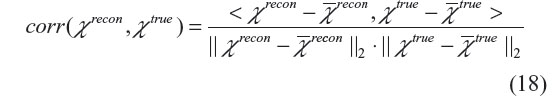
where <·,·> denotes inner production, the overbar denotes mean (or average). The pattern correlation is bounded between –1 and 1, with corr =1 representing a perfect match. For example, in the small phase angle regime we have corr(b, P) =1 due to the linear relationship in Equation 3. The 3D pattern correlation in Equation 18 is also used to numerically characterize the phantom experiments of χ tomography, where the phantom geometry defines a ground truth of χ^true.

Numerical simulations and experiment results

In the context of medical imaging development, we demonstrate the CIMRI-based χ tomography with two numerical simulations, one dye phantom experiment, and one in vivo subject brain imaging experiment. We compare two χ map reconstruction methods: inverse filtering with a truncated filter and TV iteration with a split Bregman algorithm.

Numerical simulation of cylindrical χ reconstruction

We defined a cylindrical χ source (ground truth) in a field of view (FOV) using a 3D matrix of 64 × 64 × 64 voxels, in which the cylinder is located along a central axis with a diameter of 16 voxels. Assuming that the cylinder axis is perpendicular to a main field B₀(=3T), we calculated its χ-induced fieldmap by 3D convolution in Equation 1, in which we added a 3D Gaussian noise (noise level =0.1). By T2*MRI simulation, the fieldmap can be obtained from the T2* phase image with a scale difference. From the 3D fieldmap, we reconstruct χ by solving the 3D deconvolution in Equation 4 by three methods: filter truncation in Equation 5 (denoted by ‘trunc recon’), 2-subproblem split TV iteration in Equation 12 (denoted by ‘TV2 recon’), and 3-subproblem split TV (denoted by ‘TV3 recon’).¹³ The reconstruction results are shown in Figures 1 and 2. The reconstruction goodness measures for ‘trunc recon’, ‘TV3 recon’, and ‘TV2 recon’ are 0.790, 0.996, 0.995, respectively (calculated by Equation 18). It is seen that both TV3 and TV2 could produce similar reconstructions that almost reproduce the predefined truth (corr>0.99). In what follows, we only provide the susceptibility reconstruction by the ‘TV2 recon’ method (denoted by ‘TV recon’ henceforth) without the repetition of ‘TV3 recon’, and provide the comparison with ‘trunc recon’.

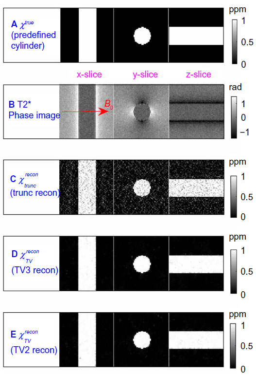Figure 1 Numerical simulation results of cylindrical magnetic susceptibility reconstructions. The 3D cylindrical volumes are displayed with three orthogonal central slices (x-slice, y-slice, and z-slice). (A) A predefined cylindrical susceptibility map (ground truth). (B) T2* phase image (calculated by T2*MRI simulation). Note that the main field B0 (marked in red arrow) is perpendicular to the cylinder axis; (C) χ reconstruction by filter truncation solver (‘trunc recon’) (Equation 5 with threshold ε0=0.12); (D) χ reconstruction by TV-regularized 3-subproblem Bregman iteration solver (‘TV3 recon’);13 (E) χ reconstruction by TV-regularized 2-subproblem Bregman iteration solver (‘TV2 recon’) (Equation 12). Both TV3 recon and TV2 recon were performed with the same settings: λ=50 and 15 iterations. Abbreviations: MRI, magnetic resonance imaging; TV, total variation.

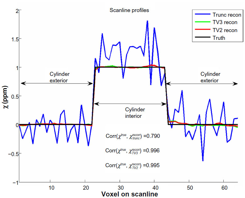Figure 2 Scan line profiles of the numerical simulations of the cylindrical susceptibility reconstructions in Figure 1. The scan line assumes a diameter of the cylinder. The ground truth is a uniform susceptibility distribution inside a cylinder, as represented by a rectangular profile. Abbreviation: TV, total variation; Trunc recon, reconstruction by filter truncation.

Numerical simulation of blob-shaped χ reconstruction

For numerical simulation of a T2*MRI capture of a dynamic brain BOLD process, we configure a cortical FOV using a support matrix of the size of 2048 × 2048 × 2048 gridels (a gridel is a grid element at a grid resolution,^32,39 which can be construed as a 1 × 1 × 1 μm³ cube in our numerical simulation) and fill the FOV with random beads (radius =3 μm) with 2% blood volume fraction. It is noted that the reason we filled the FOV with beads, instead of with random cylindrical vessels as reported previously,^13,40 was to have a good control of the 2% blood volume fraction for each cortical voxel in the cortical FOV. To simulate a local neuron stimulus on the cortical region, we defined a local Gaussian-shaped neuronal activity blob (NAB), with (σ_x, σ_y, σ_z) = (0.125, 0.125, 0.167) size (FOV), and assumed that it induces a local vascular χ perturbation by modulating the blood magnetism of cortical vasculature (random beads in our simulation). That is, we predefined a NAB-induced χ perturbation source (χ^true) using the spatial multiplication between the Gaussian distribution of the local NAB stimulus and the binary sparse volume of the bead-filled FOV, based on a linear neurovascular coupling model.⁴⁰

Considering χ^true a χ-expressed brain functional state, we carried out the T2*MRI simulation. Firstly, we calculated the 3D fieldmap (in a 3D matrix of 2048 × 2048 × 2048 gridels) using Equation 1 with B₀ =3T and an additive Gaussian noise ε(x, y, z) (with 0.1 noise level). Then, we calculated the T2* complex image (in a 3D matrix of 64 × 64 × 64 voxels) in the presence of spin diffusion⁴¹ with the following settings: T_E =30 milliseconds, δt=1 millisecond, and voxel size =32 × 32 × 32 gridels. Finally, we obtained the T2* magnitude and phase images from the T2* complex image using Equation 2. The results of the T2*MRI simulation are shown in Figure 3, in which χ^true(x, y, z) and b(x, y, z) are represented in multivoxel matrices of the size of 64 × 64 × 64 voxels.

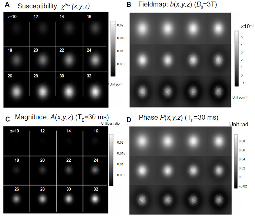Figure 3 Numerical simulation results of BOLD fMRI with a single T2* complex image acquisition by T2*MRI (a capture of dynamic BOLD processes at one time point). The 3D data matrices (at a size of 64 × 64 × 64) are displayed with a selection of z-slices (z=10:2:32 with the central z-slice at z=32) in a montage layout: (A) the predefined susceptibility source χ (see text for vascular geometry configurations); (B) the calculated fieldmap; (C) the calculated T2* magnitude image; and (D) the calculated T2* phase image. Abbreviation: BOLD fMRI, blood oxygenation level dependent functional MRI.

From the T2* phase images, we carried out χ reconstruction by implementing the filter truncation solver (threshold ε₀ =0.12, which was slightly higher than the noise level 0.1) and the TV iteration solver (λ=50). We calculated the reconstruction goodness by Equation 18 and obtained 0.99 for the TV iteration solver and 0.91 for the filter truncation solver. In Figure 4A, we show the central z-slices for the predefined χ truth and reconstructed χ maps for visual comparison. In Figure 4B, we provide scan line profiles and the pattern correlations (calculated using Equation 18) for numerical comparison. Figure 5 shows the typical iteration behavior of the split Bregman TV iteration method used for the 3D χ reconstructions. In our experience, the TV iteration algorithm converges typically in fewer than 15 iterations at an acceptable tolerance.

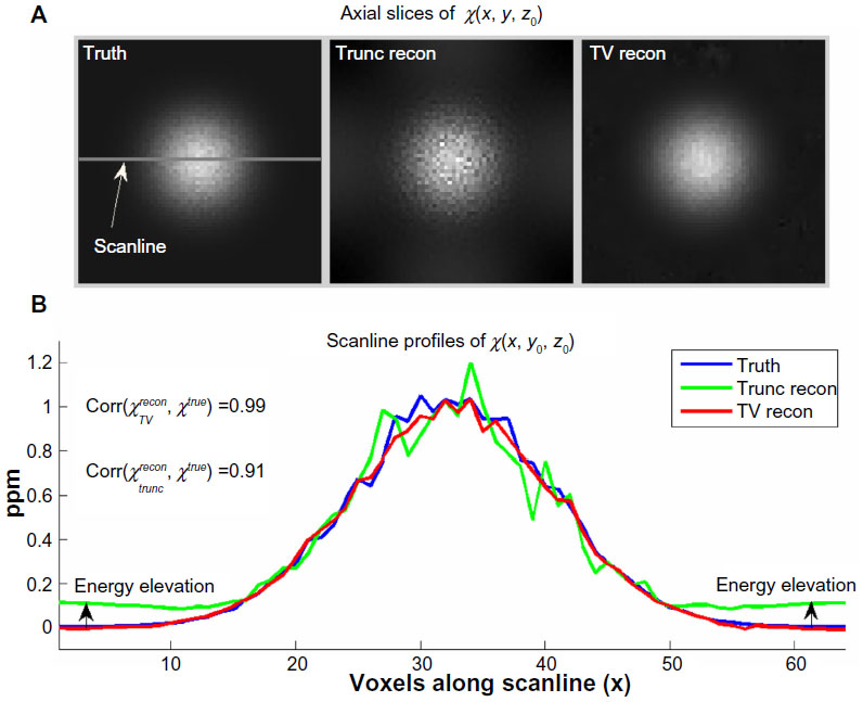Figure 4 Numerical simulation results of magnetic susceptibility reconstructions from the T2* phase images in Figure 3D by two methods: filter truncation and TV iteration. Only the central z-slices (z0=32) of the 3D 64 × 64 × 64 data matrices are shown in (A). The scan line profiles extracted from the corresponding images in (A) are shown in (B). It is noted that roughness in the predefined χ map indicates the randomness of the vascular structure in the FOV (simulated with 2% filling with random beads). The ‘trunc recon’ solver produces a noisy reconstruction with an image energy shift. The ‘TV recon’ solver produces a smooth reconstruction. The correlation values between the reconstructions and the truth (0.99 for ‘TV recon’ and 0.91 for ‘trunc recon’) were calculated using Equation 18. Abbreviations: FOV, field of view; TV, total variation; Trunc recon, truncation reconstruction.

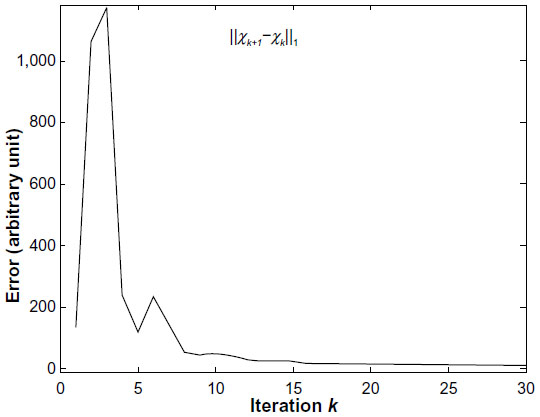Figure 5 A typical iteration behavior of the split Bregman TV iteration algorithm (with the initial setting χ1(x, y, z) = 0). Abbreviation: TV, total variation.

Phantom experiment

We created a dye phantom by adding diluted Gadolinium (Gd) dye to a plastic tube (made of polycarbonate, wall thickness =1 mm, diameter =15 mm, length =100 mm) with a 0.4 mL/30 mL dilution of clinical Gd injection (Gd concentration =287 mg/mL) in water. We used the static Gd-tube phantom to simulate a single snapshot state of a dynamic magnetic susceptibility perturbation. The Gd-tube was immersed in a water container and posed in a vertical orientation, perpendicular to the main field B₀ during scanning on a Siemens TrioTim 3T system (Munich, Germany; standard gradient-recall EPI sequence with complex output, flip angle =75°, T_E =30 milliseconds, voxel size =3 × 3 × 3 mm³). The Gd-tube provided a cylindrical χ distribution on the water background. Since we are concerned with the spatial distribution of susceptibility contrast, we normalized the susceptibility distribution of the Gd solution relative to the water background in a range of [0,1]. As a result of normalization, the Gd-tube phantom provided a binary χ distribution, χ^true χ[0,1] in dimensionless units, which is different from the distribution of absolute χ values (in units of ppm) by a constant scale. Along a scan line across a cylinder diameter, the Gd-tube phantom provides a ground truth of 1D rectangular χ distribution relative to the water background. The experiment output was a complex-valued image in a matrix of 32 ×32 ×32 voxels. From the phase image, we calculated the interim fieldmap and then calculated the source χ using both the filter truncation and TV iteration solvers. The image results are shown in Figure 6A and the scan line profiles along a tube diameter are shown in Figure 6B. The reconstruction goodness is 0.98 for the TV iteration solver and 0.91 for the filter truncation solver (calculated using Equation 18). We should point out that this Gd-tube phantom experiment was intended to justify the numerical simulation of cylindrical χ reconstruction (see Figure 1). To avoid the phase wrapping problem, we needed to dilute the clinical Gd injection such that the T2* phase image in Figure 6B remained phase unwrapped (|P(x, y, z)|<π). It is noted in Figure 6 that the left-hand side (water region) of χ^recon is slightly lower than the right-hand side (water region), which was due to imperfect field shimming over the FOV, as indicated by the unevenness of the T2* magnitude (that is, the left side appears to be slightly lifted relative to the right side). Upon this observation, we attributed the unexpected slopes in χ^recon (both inside and outside the tube regions) to the systematic experimental error (eg, imperfect field shimming) during the phantom scanning, not to the reconstruction algorithms.

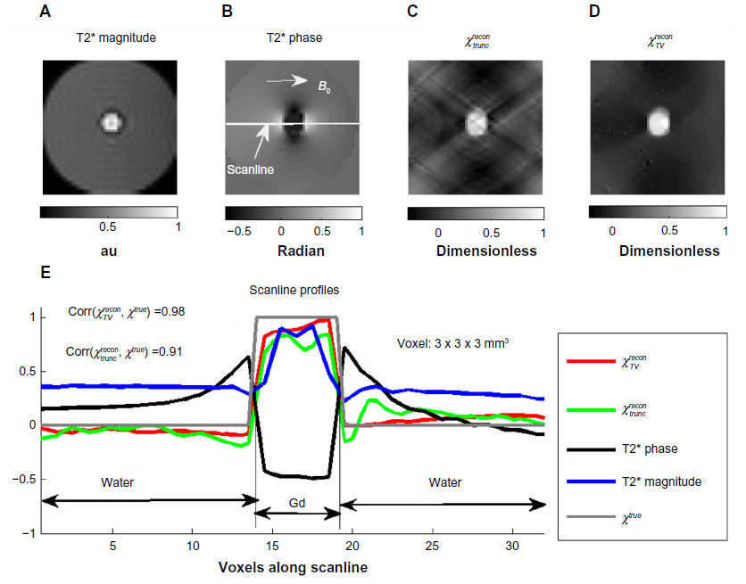Figure 6 Magnetic susceptibility reconstructions of a phantom experiment. Experiment setting: B0=3T, FOV matrix: 32 × 32 × 32 voxels, voxel size: 3 × 3 × 3mm3, phantom: a round water tank containing a Gd-filled tube (diameter =15 mm, length =100 mm), scanning direction: B0 is perpendicular to the tube axis. The data matrices (at a size of 32 × 32 × 32) are displayed with the central z-slices (z=16) in (A) for the T2* magnitude image in dimensionless arbitrary units (au); (B) the T2* phase image in units of radian; (C) the reconstructed χ map by ‘trunc recon’; and (D) the reconstructed χ map by ‘TV recon’, where the reconstructed susceptibility values in units of ppm are different from the absolute values by an undefined constant scale. The scan line profiles from the corresponding z-slices in (A) through (D) are plotted in (E). The scan line assumes a diameter of the water container (through a plastic tube diameter as marked in B). The uniform diluted Gd solution inside the tube defines a ground truth of rectangular susceptibility distribution (normalized to [0,1] by scaling) along the scan line. The reconstructed χ values are represented in dimensionless units due to normalization. The corr values (calculated in Equation 18) represent the goodness of χ reconstructions. Abbreviations: FOV, field of view; TV, total variation.

Subject experiments

Figure 7 provides a human subject experiment for in vivo brain χ tomography. The T2* complex images were acquired with a complex-enabled gradient-recall EPI sequence by scanning a healthy human brain performing a finger tapping task in a Siemens TrioTim 3T scanner, with a task paradigm: five repetitions of ‘30 seconds off | 30 seconds on’ pattern. The experimental settings were as follows: T_R/T_E =2000/29 milliseconds, B₀=3T, flip angle =75°, voxel size =2 ×2 × 2 mm³, FOV =256 × 256 × 60 mm³ in the primary motor cortex, pixel bandwidth =2,170 Hz, GRPPA reconstruction of 12-channel Head Matrix coils, B₀ // superior–inferior axis.

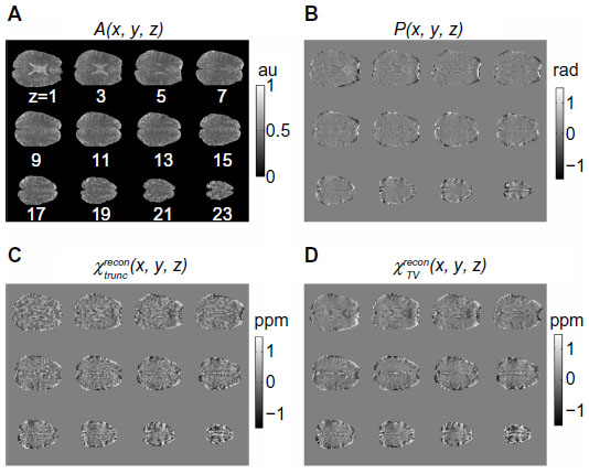Figure 7 An in vivo brain χ tomography experiment. The MRI scanning on a healthy subject performing finger tapping in a Siemens 3T TrioTim System produced both magnitude and phase time series images (EPI sequence, TR/TE =2000/29 milliseconds, voxel =2 × 2 × 2 mm3, FOV =256 × 256 × 60 mm3), image matrix: 128 × 128 × 30. (A) Magnitude image volume at a snapshot captured at an onset =20TR in the time series dataset; (B) phase image volume (processed); (C) brain χ volume reconstructed by filter truncation solver (Equation 5, with ε0 =0.12); and (D) brain χ reconstructed by TV iteration solver (Equation 12, with λ =60 and γ1 =5). Notes: Units: au (arbitrary units), rad (radian), ppm (parts per million in SI metric). Only 12 z-slices out of 128 × 128 × 30 data matrices are montage displayed (with the z labels in A). Abbreviations: FOV, field of view; TV, total variation.

We normalized the T2* magnitude images using [0,1] to produce a representation in dimensionless arbitrary units, and converted the T2* phase images using Equation 2 into a representation in units of radian and in range of (-pi, pi). From the 3D magnitude image, we calculated a 3D volume mask by thresholding with a threshold of 0.20. By spatially multiplying the 3D mask, we excluded the airspace outside the brain (setting to 0). For the 3D phase image, we performed a complex division on the 4D complex-valued fMRI dataset (dividing the complex time series dataset using the complex image from the starting time point) to reduce the phase wrapping effect.^42,43 In Figure 7A and B are respectively shown the preprocessed magnitude and phase images with a snapshot capture at an onset =20T_R out of 150 time points, where 12 z-slices out of 128 × 128 × 30 data matrices are montage displayed. It is noted in Figure 7B that inside the brain interior, the phase image takes on small values (|P|<0.3 rad), and that at the anterior and posterior boundaries, the phase image suffers from large values (|P|>1 rad) resulting from residual air/tissue interface effects during complex-division processing.

Based on the linear identity between phase and fieldmap in Equation 3, we proceeded to reconstruct 3D χ maps using both the filter truncation solver (in Equation 5 with threshold ε₀ =0.12) and the TV iteration solver (in Equation 12 with λ=60 and γ₁=5). With a computer setting of Intel Core i7CPU860 @2.80 GHz, 3GB Ram, the calculation time for reconstructing a 64 × 64 × 32 χ matrix is 0.03 seconds for the filter-truncation solver and 2 seconds for the TV-iteration solver (for 15 iterations). Figure 7C and D show the reconstructed intracranial functional χ maps using two different 3D deconvolution solvers. Figure 8 displays the z-slices at z₀ =3 in Figure 7 for visual scrutiny, where the arrows indicate the air/tissue effect that occurs at the brain boundaries in the phase image and propagates to the reconstructed χ maps. It can be seen that the filter truncation solver induces gritty textural noise and the TV iteration solver produces a smooth reconstruction. It is worth mentioning that, in this particular experiment, both reconstructions suffer from air/tissue interface effects at the brain boundaries (at the anterior and posterior regions in Figure 8D) where the complex division operation cannot completely remove the phase wrapping phenomenon.

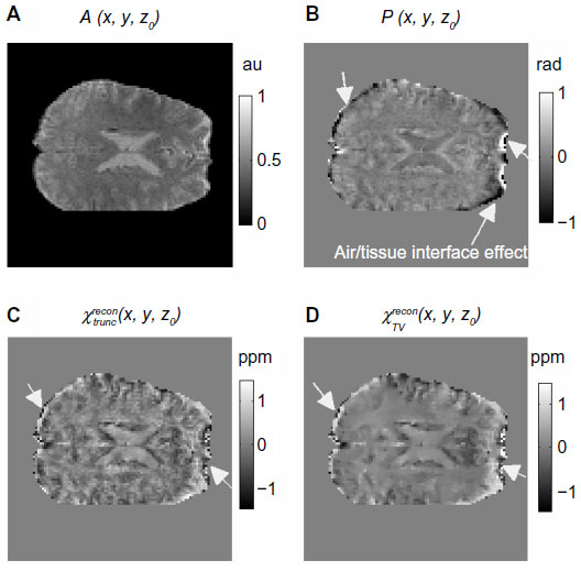Figure 8 Display of image slices at z0=3 from volumes in Figure 7: (A) magnitude image; (B) phase image (processed); (C) reconstructed χ map by filter truncation solver; and (D) reconstructed χ map by TV iteration solver. The arrows indicate air/tissue interface effects, which occur in T2* phase images and propagate to the reconstructed χ maps. Abbreviation: TV, total variation.

For an in vivo human subject experiment, the true χ distribution in the subject brain is always unknown (to be reconstructed using χ tomography), therefore, strictly speaking, we do not have the ground truth for a human brain susceptibility state that we may use to compare with the reconstructions. In principle, for tomographic medical imaging, the reconstructed χ distribution in Figures 7D and 8D can be accepted for in vivo brain state depiction as long as the brain χ tomography is well calibrated through the use of brain-tissue-equivalent phantoms.

Discussion

The main challenge of brain χ tomography lies in an ill-posed 3D deconvolution problem due to an unusual 3D bipolar-valued anisotropic kernel. The embedded zero surface of the 3D kernel manifests as a divide-by-zero problem in both matrix inverse and inverse filtering. The filter truncation method is conceptually intuitive (dealing with the 3D zero surface of dipole filter in Fourier domain) and computationally simple (data manipulation by element-wise division during 3D inverse filtering). However, this reconstruction method suffers from certain types of noises (eg, uniform random textural patterns), as demonstrated in Figure 1 with numerical simulations, in Figure 6 with a phantom experiment, and in Figure 7D with a subject experiment.

Based on numerical simulations, we conclude that the split Bregman TV iteration solver outperforms the filter truncation solver in the following aspects: 1) it denoises the data while preserving edges, therefore there is no need to smooth an MR phase image (note that the TV iteration method was originally developed for image denoising⁴⁴ and that smoothing is prone to suppressing image features and incurs irreversible information loss); 2) it is an iterative algorithm that is of numerical stability, and in particular, the split Bregman iteration ensures a fast convergence;^23,25,45 3) it is insensitive to the setting of regularization parameters due to the minimization searching of TV iterations. In our experience, the setting of λ=[30,500] could produce similar iteration results.¹³ Based on numerical simulations (in Figures 1 and 2), we show that both 3-subproblem split Bregman iteration algorithm¹³ and the 2-subproblem split algorithm in Equation 12 reveal similar convergence, λ-selection dependence, and reconstruction performance. The 2-subproblem split is preferable for its easy implementation.

In a small phase angle regime, all the phase values are small and unwrapped, such that the phase image differs from the fieldmap by a T_E-dependent factor (related by the Larmor law; see Equation 3). The small phase angle condition may be invalid for long T_E, high field B₀, and high spatial resolution.⁴⁶ For whole brain imaging, the phase wrapping phenomenon primarily occurs in sinus/tissue and air/brain boundary regions. In our subject finger tapping experiments, we were concerned with the primary motor cortex in the parietal lobe, where the T2* phase image using the complex-enabled EPI sequence (with T_E =30 milliseconds, B₀ =3T) maintains phase unwrapping (|P|<π). During T2* phase image processing, we excluded the extra-cranial airspace by 3D masking (with a binary mask volume calculated from the magnitude image volume). For fMRI dataset processing, we performed complex division to find the relative phase changes, which serves three purposes: 1) to remove the static brain χ distribution for functional brain χ tomo-graphy, 2) to remove the phase wrapping phenomenon if it existed; and 3) to reduce the static background field effect. From a time series of T2* phase images (4D dataset), 4D brain χ tomography can be implemented by repeating the 3D χ reconstruction for each snapshot volume. Obviously, this practice demands tremendous computation cost. Under the linear T2*MRI model, the susceptibility-based brain functional mapping can be calculated from the phase action map by rendering a 3D deconvolution only once, without repeating 3D χ map reconstructions for all the time points.³³ In comparison, the brute-force 4D χ tomography (based on individual 3D χ tomography at snapshots) is in general applicable for T2*MRI-based MRI datasets, not subject to the linear MRI data acquisition condition.

For large phase angle scenarios, the linear approximation in Equation 3 is not well held for calculating the interim fieldmap from the output T2* phase image due to the emergence of high-order nonlinearity in the spin precession signal expansion. A very large phase angle (|P|>π) can incur a phase wrapping phenomenon that must be corrected (by a phase unwrapping algorithm) for fieldmap calculation.⁶ For brain functional imaging, the complex division on phase image processing can reduce the phase wrapping effect to some extent. However, it cannot completely remove large phase jumps at the air/tissue interface at brain boundaries (see Figures 7B and 8B). The residual of the air/tissue interface effect due to incomplete phase image processing will propagate to the reconstructed χ maps (see Figures 7D and 8D). The T2* phase nonlinearity and air/tissue interface effect are practical aspects of brain χ tomography, which deserve further investigation.

In this report, we are concerned with functional brain χ tomography for each snapshot in an fMRI dataset. The complex division operation may largely remove static information during phase image processing. The dynamic information (including neurovascularly-coupled BOLD perturbation and inherent physiological oscillation) is retained in the processed phase images, and it will propagate to the reconstructed χ dataset. Upon the dynamic χ dataset, we can render χ-depicted functional brain mapping and investigate the cardiac and respiration effect on the functional χ perturbation using statistical χ data analysis, in the same way as statistical parametric mapping (SPM) is widely adopted for fMRI data analysis. These are ongoing research topics.

Conclusion

The goal of magnetic susceptibility (χ) tomography is to reconstruct the internal magnetic susceptibility distribution of an object from T2* phase images (as acquired by T2*MRI experiments) by rendering a computed inverse T2*MRI procedure (as described in the framework of computed inverse MRI: CIMRI).¹³ The core technology of CIMRI consists of solving a 3D ill-posed deconvolution problem, for which we have reported on a 3D total variation (TV) minimization method with a 3-subproblem split Bregman iteration algorithm in Chen and Calhoun¹³ and in this paper we report on a 2-subproblem split Bregman iteration algorithm for easy implementation. Based on numerical simulations and phantom experiments, we show that the 3D χ tomography can be successfully implemented by the TV iteration solver (source reproduction ≈99% in terms of pattern correlation). By reproducing the intact internal χ distribution from the acquired T2* phase image, brain χ tomography provides a new χ data space for more direct and truthful brain state depiction due to the removal of dipole effect and other transformations introduced during T2* image acquisition.

In this report, we claim that the internal magnetic susceptibility distribution can be reconstructed from T2* phase images (called brain χ tomography) by solving the dipole inversion problem using a TV-regularized split Bregman iteration algorithm. This claim is applicable for T2*MRI data acquisition in small phase angle condition. For more general practical applications, the T2* phase image may suffer from air/tissue interface effect and phase-wrapping phenomenon, which should be removed for the interim fieldmap calculation and the final χ calculation. Another practical aspect of brain χ tomography is the system calibration through the use of brain-tissue-equivalent phantom experiment.

Acknowledgment

This work was in part supported by NSF grants #0715022 and 0840895.

Disclosure

The authors report no conflicts of interest in this work.

---

References

1.	Chavhan GB, Babyn PS, Thomas B, Shroff MM, Haacke EM. Principles, techniques, and applications of T2*-based MR imaging and its special applications. Radiographics. 2009;29(5):1433–1449.
2.	Ogawa S, Tank DW, Menon R, et al. Intrinsic signal changes accompanying sensory stimulation: functional brain mapping with magnetic resonance imaging. Proc Natl Acad Sci U S A. 1992;89(13):5951–5955.
3.	Ogawa S, Menon RS, Tank DW, et al. Functional brain mapping by blood oxygenation level-dependent contrast magnetic resonance imaging. A comparison of signal characteristics with a biophysical model. Biophys J. 1993;64(3):803–812.
4.	Boxerman JL, Hamberg LM, Rosen BR, Weisskoff RM. MR contrast due to intravascular magnetic susceptibility perturbations. Magn Reson Med. 1995;34(4):555–566.
5.	de Rochefort L, Liu T, Kressler B, et al. Quantitative susceptibility map reconstruction from MR phase data using Bayesian regularization: validation and application to brain imaging. Magn Reson Med. 2010;63(1):194–206.
6.	Haacke EM, Tang J, Neelavalli J, Cheng YC. Susceptibility mapping as a means to visualize veins and quantify oxygen saturation. J Magn Reson Imag. 2010;32(3):663–676.
7.	Liu J, Liu T, de Rochefort L, et al. Morphology enabled dipole inversion for quantitative susceptibility mapping using structural consistency between the magnitude image and the susceptibility map. Neuroimage. 2012;59(3):2560–2568.
8.	Schweser F, Deistung A, Lehr BW, Reichenbach JR. Quantitative imaging of intrinsic magnetic tissue properties using MRI signal phase: an approach to in vivo brain iron metabolism? Neuroimage. 2011;54(4):2789–2807.
9.	Schweser F, Sommer K, Deistung A, Reichenbach JR. Quantitative susceptibility mapping for investigating subtle susceptibility variations in the human brain. Neuroimage. 2012;62(3):2083–2100.
10.	Shmueli K, de Zwart JA, van Gelderen P, Li TQ, Dodd SJ, Duyn JH. Magnetic susceptibility mapping of brain tissue in vivo using MRI phase data. Magn Reson Med. 2009;62(6):1510–1522.
11.	Wharton S, Bowtell R. Whole-brain susceptibility mapping at high field: a comparison of multiple- and single-orientation methods. Neuroimage. 2010;53(2):515–525.
12.	Wharton S, Schafer A, Bowtell R. Susceptibility mapping in the human brain using threshold-based k-space division. Magn Reson Med. 2010;63(5):1292–1304.
13.	Chen Z, Calhoun V. Computed inverse resonance imaging for magnetic susceptibility map reconstruction. J Comput Assist Tomogr. 2012;36(2):265–274.
14.	Sepulveda NG, Thomas IM, Wikswo JP. Magnetic susceptibility tomography for three-dimensional imaging of diamagnetic and paramagnetic objects. IEEE Trans Magnetics. 1994;30(6):5062–5069.
15.	Chen Z, Calhoun V. 4D Magnetic Susceptibility Tomography for Susceptibility-Based Functional Imaging. Seattle, WA: Organization for Human Brain Mapping; 2013; #1934.
16.	Chen Z, Chen Z, Calhoun VD. Voxel magnetic field disturbance from remote vasculature in BOLD fMRI. In: Pelc NJ, Samei E, Nishikawa RM, editors. Physics of Medical Imaging. Orlando, FL: SPIE Physics in Medical Imaging; 2011; #79613x.
17.	Li L, Leigh JS. Quantifying arbitrary magnetic susceptibility distributions with MR. Magn Reson Med. 2004;51(5):1077–1082.
18.	Liu T, Liu J, de Rochefort L, et al. Morphology enabled dipole inversion (MEDI) from a single-angle acquisition: comparison with COSMOS in human brain imaging. Magn Reson Med. 2011;66(3):777–783.
19.	Kressler B, de Rochefort L, Liu T, Spincemaille P, Jiang Q, Wang Y. Nonlinear regularization for per voxel estimation of magnetic susceptibility distributions from MRI field maps. IEEE Trans Med Imag. 2010;29(2):273–281.
20.	Schweser F, Deistung A, Lehr BW, Reichenbach JR. Differentiation between diamagnetic and paramagnetic cerebral lesions based on magnetic susceptibility mapping. Med Phys. 2010;37(10):5165–5178.
21.	Li W, Wu B, Liu C. Quantitative susceptibility mapping of human brain reflects spatial variation in tissue composition. Neuroimage. 2011;55(4):1645–1656.
22.	Cai J, Osher S, Shen Z. Split Bregman methods and frame based image restoration. Multiscale Model Simul. 2009;8(2):337–369.
23.	Goldstein T, Osher S. The split Bregman method for L1-regularized problems. SIAM J Imaging Sci. 2009;2(2):323–343.
24.	Osher S, Burger M, Goldfarb D, Xu J, Yin W. An iterative regularization method for total variation-based image restoration. Multiscale Model Simul. 2005;4(2):30.
25.	Vogel CR, Oman ME. Fast, robust total variation-based reconstruction of noisy, blurred images. IEEE Trans Image Process. 1998;7(6):813–824.
26.	Chambolle A, Lions PL. Image recovery via total variational minimization and related problems. Numer Math. 1997;76:22.
27.	Chan T, Esedoglu S, Park F, Yip A. Recent developments in total variation image restoration. In: Paragios N, Chen Y, Faugeras O, editors. Handbook of Mathematical Models in Computer Vision. New York: Springer; 2005.
28.	Combettes PL, Pesquet JC. Image restoration subject to a total variation constraint. IEEE Trans Image Process. 2004;13(9):1213–1222.
29.	Cheng YC, Neelavalli J, Haacke EM. Limitations of calculating field distributions and magnetic susceptibilities in MRI using a Fourier based method. Phys Med Biol. 2009;54(5):1169–1189.
30.	Reitz JR, Milford FJ, Christy RW. Foundations of Electromagnetic Theory. New York: Addison-Wisley; 1993.
31.	Chen Z, Calhoun V. Volumetric Computational Model for Neurovascular Coupling and BOLD fMRI. Quebec, CA: Organization for Human Brain Mapping; 2011.
32.	Chen Z, Calhoun VD. Magnitude and phase behavior of multiresolution BOLD signal. Concepts Magn Reson. 2010;37B(3):129–135.
33.	Chen Z, Liu J, Calhoun VD. Susceptibility-based functional brain mapping by 3D deconvolution of an MR-phase activation map. J Neurosci Methods. 2013;216(1):33–42.
34.	Chen Z, Calhoun VD. Two pitfalls of BOLD fMRI magnitude-based neuroimage analysis: non-negativity and edge effect. J Neurosci Methods. 2011;199(2):363–369.
35.	Liu T, Spincemaille P, de Rochefort L, Kressler B, Wang Y. Calculation of susceptibility through multiple orientation sampling (COSMOS): a method for conditioning the inverse problem from measured magnetic field map to susceptibility source image in MRI. Magn Reson Med. 2009;61(1):196–204.
36.	Yao B, Li TQ, Gelderen P, Shmueli K, de Zwart JA, Duyn JH. Susceptibility contrast in high field MRI of human brain as a function of tissue iron content. Neuroimage. 2009;44(4):1259–1266.
37.	Persson M, Bone D, Elmqvist H. Total variation norm for three-dimensional iterative reconstruction in limited view angle tomography. Phys Med Biol. 2001;46(3):853–866.
38.	Joshi SH, Marquina A, Osher SJ, Dinov I, Van Horn JD, Toga AW. MRI resolution enhancement using total variation regularization. Proc IEEE Int Symp Biomed Imag. 2009;2009:161–164.
39.	Chen Z, Calhoun V. A computational multiresolution BOLD fMRI model. IEEE Trans BioMed Eng. 2011;58(10):2995–2999.
40.	Chen Z, Calhoun V. Volumetric BOLD fMRI simulation: from neurovascular coupling to multivoxel imaging. BMC Med Imag. 2012;12:8.
41.	Chen Z, Calhoun V. Computed diffusion contribution in the complex BOLD fMRI signal. Concepts Magn Reson. 2012;40A(3):128–145.
42.	Arja SK, Feng Z, Chen Z, et al. Changes in fMRI magnitude data and phase data observed in block-design and event-related tasks. Neuroimage. 2009;59(4):14.
43.	Feng Z, Caprihan A, Blagoev KB, Calhoun VD. Biophysical modeling of phase changes in BOLD fMRI. Neuroimage. 2009;47(2):540–548.
44.	Rudin L, Osher S, Fatemi E. Nonlinear total variation based noise removal algorithms. Physics D. 1992;60:259–268.
45.	Joshi SH, Marquina A, Osher SJ, et al. Edge-enhanced image reconstruction using total variation and Bregman refinement. Lect Notes Comput Sci. 2009;5567:389–400.
46.	Chen Z, Chen Z, Calhoun VD. Blood oxygenation level-dependent functional MRI signal turbulence caused by ultrahigh spatial resolution: numerical simulation and theoretical explanation. NMR Biomed. 2013;26:248–264.