Prediction of cardiovascular outcomes with machine learning techniques: application to the Cardiovascular Outcomes in Renal Atherosclerotic Lesions (CORAL) study

Introduction

We have known for some time that atherosclerotic renal artery stenosis (ARAS) increases the risk of kidney function decline leading to chronic kidney disease (CKD), cardiovascular disease, and death.^1–3 However, the effect of renal artery revascularization by stenting on renal and cardiovascular outcomes is inconsistent. Specifically, two large randomized controlled trials, namely the ASTRAL and Cardiovascular Outcomes in Renal Atherosclerotic Lesions (CORAL) studies, have demonstrated virtually identical outcomes in patients treated with medical therapy alone or medical therapy plus stenting.^4,5 That said, it is very clear that patients may have very different responses to renal artery stenting, leading many clinicians to believe that prediction of responses to renal artery stenting may be possible. One of the challenges for the completion of the CORAL study was the difficulty of convincing physicians at participating centers that there was, in fact, equipoise regarding the utility of stenting across the varied clinical presentations of ARAS. While convincing the physicians of equipoise was difficult, careful analysis of the CORAL data set to date has not yielded clinical scenarios where medical therapy plus stenting was either markedly better or worse than medical therapy alone.

On this background, there are a number of machine learning methods which can be applied to clinical data sets. A few studies have recently reported on the utility of these methods for predicting renal outcomes in the classic MDRD study.⁶ To the best of our knowledge, neither CORAL nor ASTRAL data sets have been analyzed with machine learning approaches. With the idea that these machine learning methods might discern patterns which are opaque to routine clinical judgment, the following reanalysis of the CORAL data set was undertaken.

Methods

CORAL trial

CORAL is a prospective, international, multicenter clinical trial that randomly assigned 931 participants with ARAS who received optimal medical therapy to stenting vs no stenting. Enrollment began on May 16, 2005 and concluded on January 30, 2012 with follow-up until September 28, 2012, at which time study objectives were accomplished and statistical power was sufficient for the primary trial outcome analyses. The study protocol adhered to the principles of the Declaration of Helsinki and was approved by the institutional review boards (IRBs) or the ethics committees at each participating site. A list of these IRBs can be found in the IRB supplement. All participating subjects provided written informed consent. Participants with ARAS were randomized in a 1:1 ratio to medical therapy plus stenting or medical therapy alone. Neither participants nor the investigators or the study coordinators were blinded to group assignment. Both groups received anti hypertensive therapy with a stepwise approach to achieve the blood pressure target, starting with an angiotensin receptor blocker or an angiotensin-converting-enzyme inhibitor.

The primary endpoint for CORAL, as well as for the current study, was the first occurrence of a major cardiovascular or renal event – this was a composite of death from cardiovascular or renal causes, stroke, myocardial infarction, hospitalization for congestive heart failure, progressive renal insufficiency or need for renal replacement therapy. Detailed study entry criteria and main outcomes of this trial have been published.⁵ Patients with renal artery stenosis of at least 60% were eligible if they had hypertension while receiving two or more antihypertensive agents or had an estimated glomerular filtration rate (eGFR) <60 mL/min/1.73 m². Angiograms were analyzed for verification of stenosis by the Angiography Core Lab for the study at the University of Virginia.

Statistical analyses

All analysis was performed using the open source program R.⁷ Although 931 patients were present in the initial data set, many of these patients had missing values (especially baseline laboratory values). The data were cleaned by excluding variables with large numbers of missing values (>40% missing values). Variables with more moderate amounts of missing values that had numeric data had the average value placed into missing value categories (<20% missing values). Missing non-numerical data (eg, race, gender, smoking) caused us to drop the subjects from further analysis. Analysis of 573 subjects with complete records was then performed. The R code was employed to clean these data as shown in Supplementary material 1. Parameters used for subsequent analysis are shown in Box 1. Before analyzing the data set without missing values, multiple methods of imputation for both missing categorical and continuous data were employed and yielded results were similar to the results of analysis of the cleansed data (data not shown).

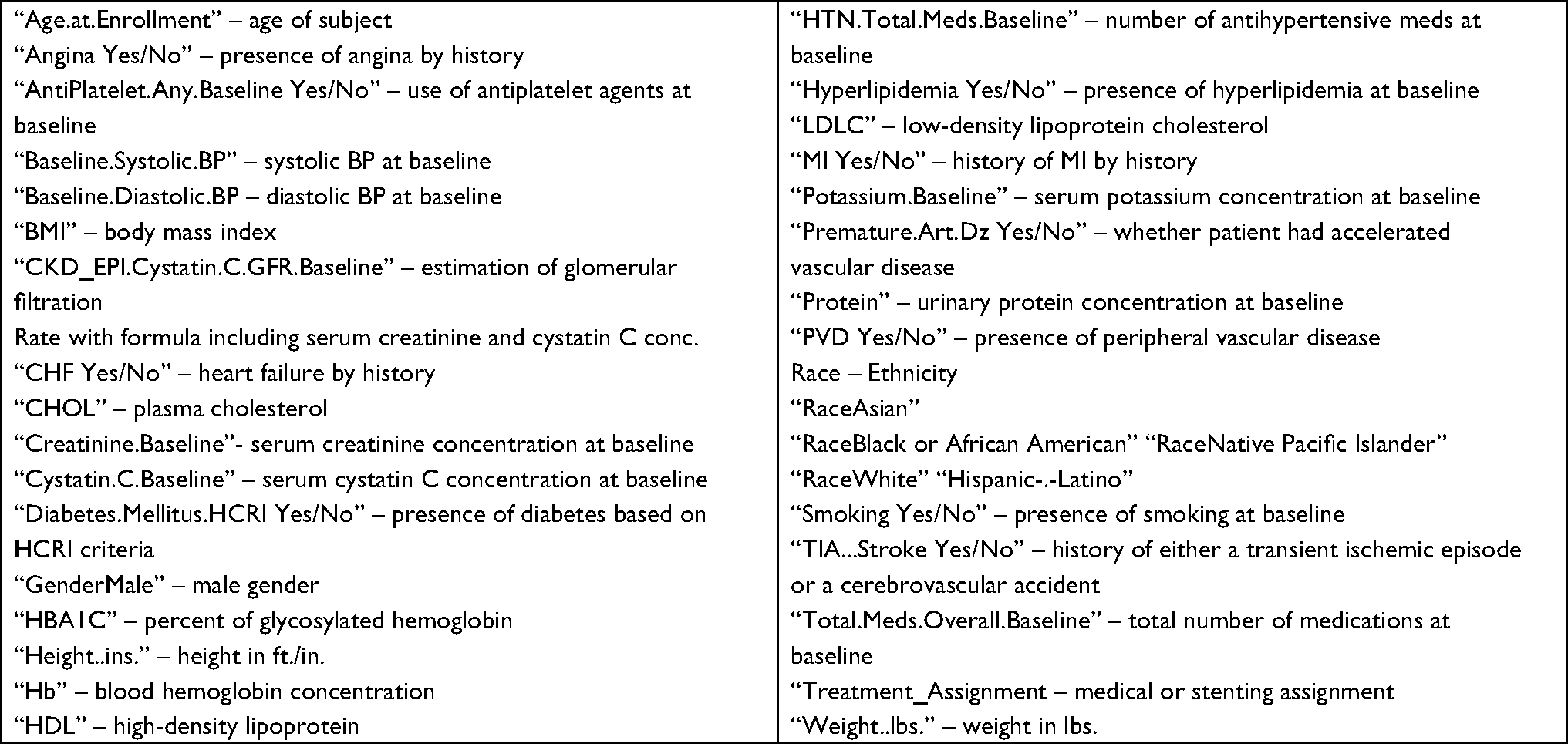Box 1 Data used for predictive models. Abbreviations: MI, myocardial infarction; MI, myocardial infarction; CKD, chronic kidney disease; conc., concentration; HCRI, Harvard Clinical Research Institute.

Logistic regression and support vector machine

We used a generalized linear (logistic regression) model our default⁸ using only baseline variables for the prediction of composite endpoint outcomes. In addition, we examined the utility of a support vector machine (SVM) which involves the multidimensional sorting of data based on the development of a hyperplane which best segregates the two classes.⁸ Using the CARET package,⁹ we employed two tuning parameters to control the performance of the SVM: kernel and C. Kernel is a complex function, which takes input from a lower dimension and transforms it to a higher dimension, and is useful in a nonlinear separation problem. We used the radial kernel option from the CARET package. When radial kernel is applied, one additional parameter, Sigma, needs to be specified, since higher values of Sigma tend to cause an over-fitting problem. The second tuning parameter used was C, which is a regularization parameter and specifies the penalty for misclassification. Larger values of C indicate a larger misclassification penalty, and thus, the optimization will choose a hyperplane that separates cases with as small a margin of misclassification as possible. Alternatively, a smaller value of C would yield a larger-margin separating hyperplane, even if it misclassifies more points compared with smaller-margin hyperplane. The best combination of C and Sigma values is determined using cross-validation.¹⁰ Sigma and C values were optimized within the CARET package, and values of 1e-3 and 32 were used thereafter.

Random forest

The third method we applied is the random forest, which employs decision trees to construct a predictive model using a set of binary rules applied to calculate a target value.¹¹ It can be used for both classification and regression. The decision tree approach utilized three or more nodes. Random forest uses a tree-based resembling method for reducing bias and combines (average) the results from many decision tree models obtained by bootstrap samples. There are two tuning parameters for the random forest: the number of trees (ntree) we would like to average and the number of variables (mtry) randomly sampled as candidates at each split in each tree. We examined the performance of decision trees with the RPART package and random forests with the randomForest package.^12,13 With the random forest technique, ntree was set at 1,000 and mtry was optimized at 9.

Neural network

We also tried a feed-forward neural network.¹⁴ Neural network passes information through multiple layers of processors. Similarly, neural network takes input from the data forming the bottom layer, processes it through multiple neurons from multiple hidden layers, and returns the result forming the top layer. The outputs of nodes in one layer are inputs to the next layer where the inputs to each node are combined using a weighted linear combination. Three tuning parameters are needed: one is the number of hidden layers, the second one is the number of nodes in each hidden layer, and the third one is the decay parameter. The decay parameter restricts the weighting from being too large. Different feed-forward neural network architectures were explored using the nnet and neuralnet packages.¹⁵ We found optimal performance with one hidden layer containing nine hidden neurons with a decay value of 0.24 after initial exploration.

Model comparisons

The CARET package was used for comparison of the mature models employing ten folds and three repeats.^9,16 Other packages within R were used for different specific tasks (eg, nnet for construction of the neural network and random forest [randomForest] for constructing random forests).^7,11,15–24 All numerical data were centered and scaled prior to analysis with all of the above methods. The R code used for these analyses is shown in Supplementary material 2.

Training and test sets

In the first phase, we varied the tuning parameters on a training subset with the CARET package. For all analyses, three repeats of the ten folds were used. For the SVM, the Sigma and C values were varied from 0.1 to 1. Once these parameters were optimized for the different methods, we used different seed values to split the training and testing sets (80% training:20% testing). We then employed the strategy of three repeats of the ten-folds with CARET on the different training subsets achieved, varying the seed to initiate randomization to divide the set into training and testing subsets. Areas under the curve for the receiver operator curve (ROC) were improved by ~5%–7% by the inclusion of these baseline laboratory values (data not shown).

Statistical comparisons of ROC values determined with ten different seed values for splitting training and testing sets were performed on data obtained both with the training and testing sets. The overall data sets were compared with one-way ANOVA and individual group means compared using unpaired t-test with Holm–Sidak correction for multiple comparisons.⁷

Results

The results of the training and testing subsets are shown in Table 1. Although the methodologies were quite different, it was clear that all the machine learning methods except the simple decision tree yielded very similar ROC areas and accuracy values. A comparison of the ROC curves from one analysis which illustrates this is shown in Figure 1.

Table 1 ROC values achieved with training and testing sets Notes: Results expressed as mean ± SD of n=10 trials with different seed values used to split CORAL data set into training and testing subsets. Statistical comparison of both training and testing ROC by ANOVA showed it to be highly significant. Comparison of group means using Holm–Sidak correction for multiple comparisons shown with significance reported as NS, P<0.05, and P<0.01 levels. Abbreviations: CORAL, Cardiovascular Outcomes in Renal Atherosclerotic Lesions; GLM, generalized linear method; NS, nonsignificant; ROC, receiver operator curve; nnet, neural network; RF, random forest; RPART partition; SVM, support vector machine.

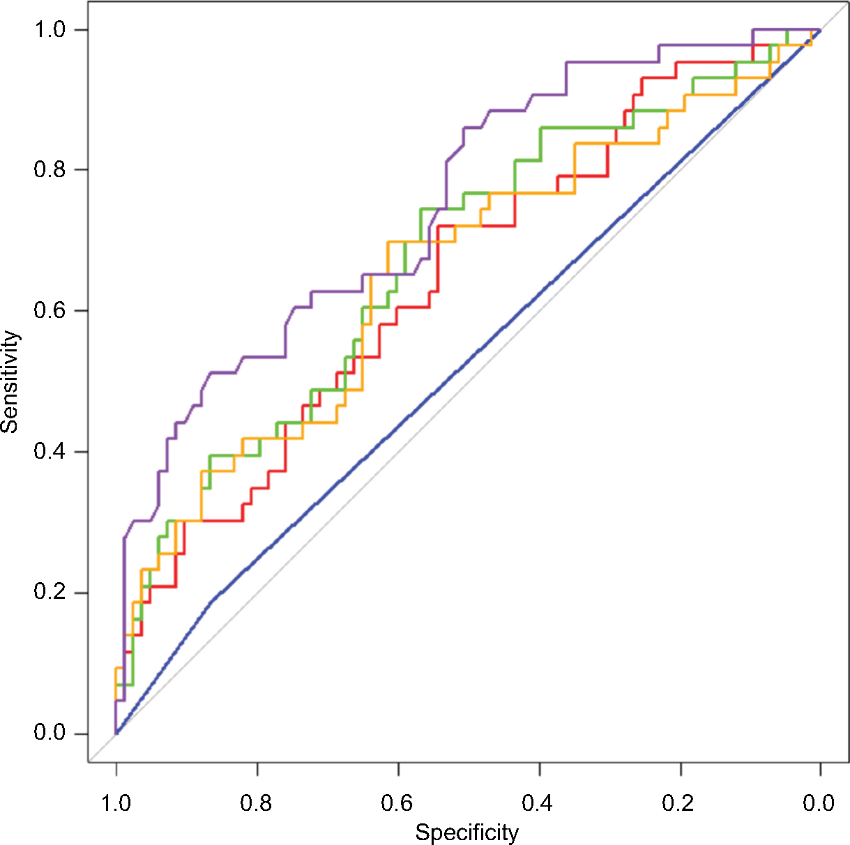Figure 1 Representative ROCs generated with different models with a seed of 2. Red is generalized linear, green the support vector machine, blue the decision tree, orange the neural network, and purple the random forest model. Abbreviation: ROC, receiver operator curve.

Representative confusion matrices are shown in Table 2. Clearly, the SVM method was very much slanted toward negative values. Balancing the training set with outcomes avoided that solution which approached the trivial, but did not improve overall accuracy (data not shown). The other methods yielded more balanced results with training set chosen randomly. The balance between sensitivity and specificity was probably the best with the neural network model (Table 2), although the random forest method yielded the highest accuracy in most of the simulations (Table 1).

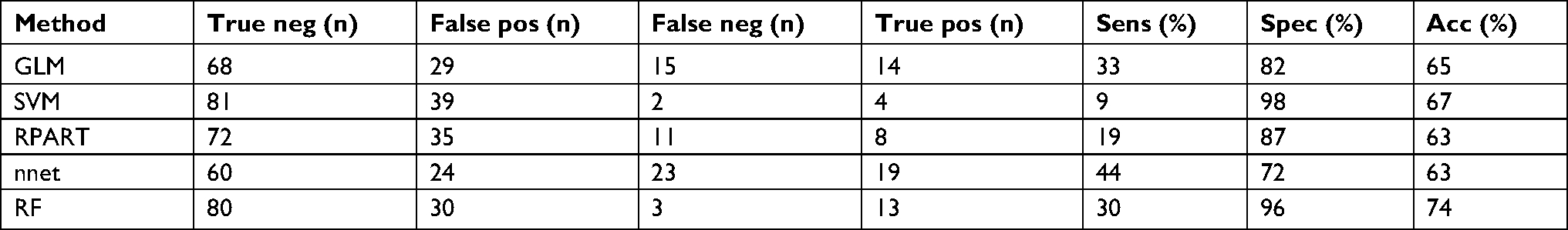Table 2 Confusion matrices in different models Notes: Results selected from analysis performed with seed 2 chosen to generate training and testing sets. Sens refers to sensitivity at detecting a composite outcome (true pos/[true pos + false neg]). Spec refers to specificity at excluding a composite outcome (true neg/[true neg + false pos]), and Acc refers to the accuracy of the assignment. Although results are only shown with seed 2, results were very similar with different seeds, varying only by a few percentage points. Abbreviations: GLM, generalized linear method; neg, negative; pos, positive; nnet, neural network; RF, random forest; RPART partition; SVM, support vector machine.

Examining the factors emphasized by the machine learning methods, it is worthwhile to note that, while different measurements were emphasized by the different techniques, the treatment assignment was not considered a strong predictor by any model (Table 3). This supports the overall conclusion of the CORAL study that stenting did not add materially to medical therapy in the avoidance of composite cardiovascular outcomes in ARAS. In contrast, the baseline SBP as well as estimates of renal function appeared to be consistently featured by the different models as top predictors of adverse outcomes. This is also consistent with the CORAL findings that, although the treatment groups were similar at baseline with regard to SBP and measures of renal function, higher SBP and lower eGFR were prevalent in subjects who experienced a composite endpoint event. While there may be some correlation among estimates of renal function, creatinine was consistently chosen as a top predictor of adverse outcomes by the models, while eGFR, based on the CKD-epidemiology collaboration cystatin C equation, was selected by only one model as the fourth in importance.

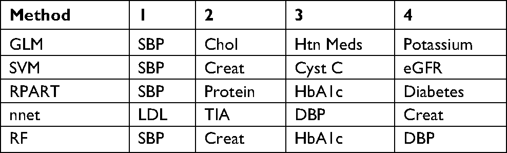Table 3 Top four important variables with different models Notes: Data derived from seed =2. Similar results with different seeds for all models. Abbreviations: Chol, cholesterol; Creat, creatinine; eGFR, estimated glomerular filtration rate; GLM, generalized linear method; HbA1c, glycated hemoglobin; Htn, hypertension; LDL, low-density lipoprotein; nnet, neural network; RF, random forest; RPART partition; SVM, support vector machine; TIA, transient ischemic attack.

Discussion

We attempted to apply machine learning methods to develop a strategy for predicting outcomes in atherosclerotic renal artery disease. The CORAL data set was used as the substrate for these methods.

Although we found that some classification methods outperformed others, the results were somewhat disappointing with ROC values generally <0.7. We would emphasize that these results were somewhat inferior to what we saw when a similar suite of machine learning methods were applied to the modification of diet in renal disease (MDRD) data set. Although the MDRD data set was somewhat larger, we expect that the clinical course of the subjects studied in the MDRD (patients with advanced CKD) was somewhat easier to predict than that of the CORAL patients.^5,6 This showed, the random forest approach generally outperformed the other methods, with the SVM having particular problems in identifying patients who achieved composite endpoints when trained with the unbalanced training set. The decision tree also performed quite poorly, and we would emphasize that this machine learning method most closely mirrors human decision making with a limited number of measurements used for categorization. This latter point along with the absence of the treatment assignment on the top predictor lists sadly supports the contention that the prediction of outcomes in patients with atherosclerotic renal artery disease based on baseline clinical parameters is not trivial, and that stenting does not materially affect outcomes in either the overall population or any clearly defined subset based on these baseline clinical parameters.

In the current analysis, urinary protein derived from the baseline urinalysis was used in our machine learning methods rather than urinary albumin creatinine ratio as reported by Murphy et al,²⁵ as there were fewer missing values. Urinary protein was not a consistently important predictor in any of the models (Table 3). On this note, SBP and creatinine were commonly included as important factors in the models studied. However, treatment group assignment was not, underlining the ineffectiveness of stenting to improve outcomes in this population.

Data sharing statement

De-identified data from the CORAL data set are available for other investigators to review or analyze on the NHLBI BioLINCC website (https://biolincc.nhlbi.nih.gov/studies/coral/?q=CORAL). Procedures for accessing these data are detailed on the BioLINCC website.

Acknowledgments

The CORAL clinical trial was supported by a grant from the National Heart, Lung, and Blood Institute (NHLBI) of the National Institutes of Health under Award Numbers U01HL071556, U01HL072734, U01HL072735, U01HL072736, and U01HL072737. Study drugs were provided by AstraZeneca and Pfizer. Study devices were provided by Cordis Corporation, and supplemental financial support was granted by both Cordis Corporation and Pfizer Inc. None of the sponsors had any role in design and conduct of the study, collection, management, analysis, and interpretation of the data, or review or approval of the manuscript. The trial was registered at ClinicalTrials.gov number, NCT00081731.

The authors express their sincere appreciation for the support and encouragement provided by Diane M Reid, MD, Medical Officer, Division of Cardiovascular Sciences, NHLBI, Bethesda, MD.

Author contributions

All authors contributed toward data analysis, drafting and critically revising the paper, gave final approval of the version to be published, and agree to be accountable for all aspects of the work. The content of this paper is solely the responsibility of the authors. TC had full access to the data. She, along with JIS wrote the R code used for machine learning and analyzed the CORAL data set with these methods. She also contributed to the writing of the manuscript. PB had full access to the data. She prepared and summarized data for subsequent machine learning analysis. She also contributed to the writing of the manuscript. KRT was responsible for study design, and conduct. LDD was involved in the design of the study, collection and analysis of data. WH provided input on data inclusion and analyses. BAG and ST contributed to review of study data. MS supervised generation of data from the research laboratory. KJ contributed to design of the present analyses, review of study data, and writing of the manuscript. KP, JMM, RBD Sr, and DEC were responsible for and conducted the data analyses. RBD Sr also contributed considerable input and review as the senior statistician for the CORAL clinical trial. DEC also made substantial contribution to study design and data acquisition along with critical review of the manuscript for intellectual content as well as final approval of the manuscript. He agrees to be accountable for all aspects of the work. TPM provided input into writing the manuscript and edited final revisions. CJC was responsible for study design and analysis, and the writing of the manuscript. JIS contributed to writing and editing the manuscript. He also served as the enrollment chairman during the performance of the CORAL trial.

Disclosure

KRT has received grants from the NHLBI and the National Institute of Diabetes, Digestive, and Kidney Diseases (NIDDK). She has received consulting fees from Eli Lilly and Company, Amgen, and Noxxon Pharma, as well as research support from Eli Lilly and Company. LDD has received grants from the National Institutes of Health (NIH) and research support from Pfizer, Astra Zeneca, and Johnson & Johnson. BAG and MS have received grants from the NIH. ST has received personal fees from AbbVie. KJ has received grants from the Medical College of Toledo. KP has received grants from the NHLBI. JMM has received personal fees from the Harvard Clinical Research Institute and grants from the NHLBI. RBD Sr has received grants from the NHLBI. DEC has received grants from the NHLBI and research support from Medtronic, Boston Scientific, and Abbott Vascular. CJC has received research funding from Cordis, study drugs from AstraZeneca, and study drugs and research funding from Pfizer. JIS has received grants from the NIH, BrickStreet Insurance Endowment, and the Huntington Foundation Endowment. The authors report no other conflicts of interest in this work.

References

1.		Conlon PJ, Athirakul K, Kovalik E, et al. Survival in renal vascular disease. J Am Soc Nephrol. 1998;9(2):252–256.
2.		Chábová V, Schirger A, Stanson AW, Mckusick MA, Textor SC. Outcomes of atherosclerotic renal artery stenosis managed without revascularization. Mayo Clin Proc. 2000;75(5):437–444.
3.		Zalunardo N, Tuttle KR. Atherosclerotic renal artery stenosis: current status and future directions. Curr Opin Nephrol Hypertens. 2004;13(6):613–621.
4.		Wheatley K, Ives N, Gray R, et al. Revascularization versus medical therapy for renal-artery stenosis. N Engl J Med. 2009;361(20):1953–1962.
5.		Cooper CJ, Murphy TP, Cutlip DE, et al. Stenting and medical therapy for atherosclerotic renal-artery stenosis. N Engl J Med. 2014;370:13–22.
6.		Khitan Z, Shapiro AP, Shah PT, et al. Predicting adverse outcomes in chronic kidney disease using machine learning methods: data from the modification of diet in renal disease. Marshall J Med. 2017;3(4):67–79.
7.		R Core Team. R: a Language and Environment for Statistical Computing. Vienna, Austria: R Foundation for Statistical Computing; 2017.
8.		Gullo CA, McCarthy MJ, Shapiro JI, Miller BL. Predicting medical student success on licensure exams. Med Sci Educ. 2015;25:447–453.
9.		Kuhn M, Wing J, Weston S, et al. CARET: classification and regression training; 2017. Available from: https://CRAN.R-project.org/package=caret. Accessed March 13, 2019.
10.		Sing T, Sander O, Beerenwinkel N, Lengauer T. ROCR: visualizing classifier performance in R. Bioinformatics. 2005;21(20):3940–3941.
11.		Liaw A, Wiener M. Classification and regression by randomForest. R News. 2002;2:5.
12.		Chen T, Cao Y, Zhang Y, et al. Random forest in clinical metabolomics for phenotypic discrimination and biomarker selection. Evid Based Complement Alternat Med. 2013;2013(11):1–11.
13.		Khondoker MR, Bachmann TT, Mewissen M, et al. Multi-factorial analysis of class prediction error: estimating optimal number of biomarkers for various classification rules. J Bioinform Comput Biol. 2010;08(06):945–965.
14.		Venables WN, Ripley BD. Modern Applied Statistics with S. New York, NY: Springer; 2002.
15.		Zhang Z. A gentle introduction to artificial neural networks. Ann Transl Med. 2016;4(19):370.
16.		Tsiliki G, Munteanu CR, Seoane JA, Fernandez-Lozano C, Sarimveis H, Willighagen EL. RRegrs: an R package for computer-aided model selection with multiple regression models. J Cheminform. 2015; 7(1):46.
17.		Liu R, Li X, Zhang W, Zhou H-H. Comparison of nine statistical model based warfarin pharmacogenetic dosing algorithms using the racially diverse international warfarin pharmacogenetic Consortium cohort database. PLoS One. 2015;10(8):e0135784.
18.		Robin X, Turck N, Hainard A, et al. pROC: an open-source package for R and S+ to analyze and compare ROC curves. BMC Bioinformatics. 2011;12(1):77.
19.		Emir B, Johnson K, Kuhn M, Parsons B. Predictive modeling of response to pregabalin for the treatment of neuropathic pain using 6-week observational data: a spectrum of modern analytics applications. Clin Ther. 2017;39(1):98–106.
20.		Hengl T, Mendes de Jesus J, Heuvelink GBM, et al. SoilGrids250m: global gridded soil information based on machine learning. PLoS One. 2017;12(2):e0169748.
21.		Gallo S, Hazell T, Vanstone CA, et al. Vitamin D supplementation in breastfed infants from Montreal, Canada: 25-hydroxyvitamin D and bone health effects from a follow-up study at 3 years of age. Osteoporos Int. 2016.
22.		Heuer C, Scheel C, Tetens J, Kühn C, Thaller G. Genomic prediction of unordered categorical traits: an application to subpopulation assignment in German Warmblood horses. Genet Sel Evol. 2016;48(1):13.
23.		Wickam H. Elegant Graphics for Data Analysis. New York, NY: Springer-Verlag; 2009.
24.		Kennedy DJ, Burket MW, Khuder SA, Shapiro JI, Topp RV, Cooper CJ. Quality of life improves after renal artery stenting. Biol Res Nurs. 2006;8(2):129–137.
25.		Murphy TP, Cooper CJ, Pencina KM, et al. Relationship of albuminuria and renal artery stent outcomes: results from the coral randomized clinical trial (cardiovascular outcomes with renal artery lesions). Hypertension. 2016;68(5):1145–1152.

Supplementary materials

Supplementary material 1: Data import and cleaning

setwd(“C:/Users/shapiroj/Dropbox/Current Stuff/work”)

library(dplyr)

dat <- read.csv(“temp_coral_v3c.csv”,stringsAsFactors=FALSE,na.string=c(“”,NA,” “,”U”,”Unk”))

dim(dat)

dat1 = dat[,!apply(is.na(dat), 2, all)] # automatically get rid of empty cols at the end

dim(dat1)

# get rid of time to event days and make outcome yes or no

k1 = ncol(dat1)-1;k1

colnames(dat1)[k1] <- “output1”

temp = dat1[,k1]

dat1[temp==1,k1] <- “yes”

dat1[temp==0,k1] <- “no”

dat1[,k1] <- factor(dat1[,k1])

dat2 <- dat1[,-ncol(dat1)] # get rid of last Days.to.Prim.Endpoint

keep <- (apply(dat2,2,function(x) sum(is.na(x))) < 400)

sum(keep)

dat_temp = dat2[,keep]

dat1=dat_temp

# merge the clinical and laboratory data

cc=colnames(dat1)[1]

# add in labs

x1=read.csv(“TG.csv”)

x2=read.csv(“CHOL.csv”)

x3=read.csv(“HBA1C.csv”)

x4=read.csv(“HDL.csv”)

x5=read.csv(“LDL.csv”)

x6=read.csv(“Hb.csv”)

# create final dataset

dat1=full_join(x1,dat1, by=cc, copy=T)

dat1=full_join(x2,dat1, by=cc, copy=T)

dat1=full_join(x3,dat1, by=cc, copy=T)

dat1=full_join(x4,dat1, by=cc, copy=T)

dat1=full_join(x5,dat1, by=cc, copy=T)

dat1=full_join(x6,dat1, by=cc, copy=T)

# clean up memory

rm(x1)

rm(x2)

rm(x3)

rm(x4)

rm(x5)

rm(x6)

# average in missing numerical data to reduce missing values

vv=c(2:8,12:14,16:21,26,28)

#

mm=NULL

for(j in 1:length(vv)){

mm[j]=mean(dat1[,vv[j]],na.rm=T)

}

for(i in 1:length(vv)){

dat1[,vv[i]][is.na(dat1[,vv[i]])]=mm[i]

}

#sum(!complete.cases(dat3))

z=dat1[complete.cases(dat1),]

z=z[,-1]

z=z[complete.cases(z),]

Supplementary material 2: Some variations used, version to determine variable importance as well as area under the curve (AUC) for receiver operator curve (ROC) and confusion matrix generation

library(ROCR)

library(pROC)

library(rpart)

library(caret)

library(nnet)

library(C50)

library(ggplot2)

library(randomForest)

# Could be run as a loop, but to avoid crashing, I ran them individually

# kk=NULL

# #run simulations and save data

# kk=c(2,14,25,33,57,61)

sink(“VIP_coral”,append=FALSE)

print(“VIP_coral”)

sink()

# seed value set for 61 below, could have been a loop

kk=61

set.seed(kk)

ind = sample(2, nrow(z), replace = TRUE, prob = c(0.8, 0.2))

trainset = z[ind == 1,]

testset = z[ind == 2,]

control = trainControl(method = “repeatedcv”, seeds=c(539, 704, 483, 253, 63, 887, 105, 65, 62, 343, 633, 870, 457, 422, 53, 189, 605, 628, 950, 781, 981, 284, 498, 198, 822, 150, 55, 166, 99, 874, 431), number = 10, repeats = 3, classProbs = TRUE, summaryFunction = twoClassSummary)

glm.model = train(output1 ~ ., data = trainset, method = “glm”, metric = “ROC”, trControl = control, preProc=c(“center”,”scale”))

t=varImp(glm.model)

sink(“VIP_coral”,append=TRUE)

print(“glm”)

print(t)

sink()

tunGrid_svm=expand.grid(sigma=1e-3, C=32)

svm.model = train(output1 ~ ., data = trainset, method = “svmRadial”,metric = “ROC”, tuneGrid=tunGrid_svm, trControl = control, preProc=c(“center”,”scale”))

t=varImp(svm.model)

sink(“VIP_coral”,append=TRUE)

print(“svm”)

print(t)

sink()

rpart.model = train(output1 ~ ., data = trainset, method = “rpart”, metric = “ROC”, trControl = control, preProc=c(“center”,”scale”))

t=varImp(rpart.model)

sink(“VIP_coral”,append=TRUE)

print(“rpart”)

print(t)

sink()

tunGrid=expand.grid(size=c(9),decay=c(0.24))

nnet.model = train(output1 ~ ., data=trainset, method = “nnet”, metric=”ROC”, trace=FALSE, trControl=control, tuneGrid=tunGrid, preProc=c(“center”,”scale”))

t=varImp(nnet.model)

sink(“VIP_coral”,append=TRUE)

print(“nnet”)

print(t)

sink()

tunegrid=expand.grid(.mtry=9)

rfor.model = train(output1 ~ ., data=trainset, method = “rf”, metric=”ROC”, trControl=control,tuneGrid=tunegrid, preProc=c(“center”,”scale”))

t=varImp(rfor.model)

sink(“VIP_coral”,append=TRUE)

print(“rfor”)

print(t)

sink()

# make ROC comparisons

glm.probs = predict(glm.model, testset[,! names(testset) %in% c(“output1”)], type = “prob”)

svm.probs = predict(svm.model, testset[,! names(testset) %in% c(“output1”)], type = “prob”)

rpart.probs = predict(rpart.model, testset[,! names(testset) %in% c(“output1”)], type = “prob”)

nnet.probs=predict(nnet.model, testset[,! names(testset) %in% c(“output1”)], type = “prob”)

rfor.probs=predict(rfor.model, testset[,! names(testset) %in% c(“output1”)], type = “prob”)

windows()

glm.ROC = roc(response = testset[, c(“output1”)], predictor = glm.probs $yes, levels = levels(testset[, c(“output1”)]))

plot(glm.ROC,add=F, col =” red”)

svm.ROC = roc(response = testset[, c(“output1”)], predictor = svm.probs $yes, levels = levels(testset[, c(“output1”)]))

plot(svm.ROC, add = TRUE, col =”green”)

rpart.ROC = roc(response = testset[, c(“output1”)], predictor = rpart.probs $yes, levels = levels(testset[, c(“output1”)]))

plot(rpart.ROC, add = TRUE, col =”blue”)

nnet.ROC=roc(response = testset[, c(“output1”)], predictor = nnet.probs $yes, levels = levels(testset[, c(“output1”)]))

plot(nnet.ROC, add = TRUE, col =”orange”)

rfor.ROC=roc(response = testset[, c(“output1”)], predictor = rfor.probs $yes, levels = levels(testset[, c(“output1”)]))

plot(rfor.ROC, add = TRUE, col =”purple”)

#make confusion matrix

print(“glm”)

glm.pred=predict(glm.model,testset[,!names(testset)%in% c(“output1”)])

t=table(glm.pred,testset[,c(“output1”)])

tt=confusionMatrix(glm.pred,testset[,c(“output1”)])

print(tt)

print(“svm”)

svm.pred=predict(svm.model,testset[,!names(testset)%in% c(“output1”)])

t=table(svm.pred,testset[,c(“output1”)])

tt=confusionMatrix(svm.pred,testset[,c(“output1”)])

print(tt)

print(“rpart”)

rpart.pred=predict(rpart.model,testset[,!names(testset)%in% c(“output1”)])

t= table(rpart.pred,testset[,c(“output1”)])

tt=confusionMatrix(rpart.pred,testset[,c(“output1”)])

print(tt)

print(“nn”)

nnet.pred=predict(nnet.model,testset[,!names(testset)%in% c(“output1”)])

t= table(nnet.pred,testset[,c(“output1”)])

tt=confusionMatrix(nnet.pred,testset[,c(“output1”)])

print(tt)

print(“rfor”)

rfor.pred=predict(rfor.model,testset[,!names(testset)%in% c(“output1”)])

t=table(rfor.pred,testset[,c(“output1”)])

tt=confusionMatrix(rfor.pred,testset[,c(“output1”)])

print(tt)