Longitudinal analysis of an antihypertensive trial comparing the single pill combination of telmisartan and amlodipine with their monotreatments

Introduction

A double-blind, Phase III clinical trial was designed to study the treatment effect of a single pill combination (SPC) of 80 mg telmisartan and 10 mg amlodipine in lowering systolic blood pressure (SBP). This was an 8-week study with three treatment groups, ie, SPC, telmisartan, and amlodipine. A forced titration schedule for amlodipine was applied, ie, patients who were randomized to amlodipine or to SPC were treated for the first 2 weeks with amlodipine 5 mg, and then titrated to 10 mg of amlodipine for another 6 weeks. A constant dose of 80 mg telmisartan was applied for the entire 8-week treatment period.

After a single-blind washout of 3–4 weeks, a total of 858 subjects with severe hypertension (SBP >180 mmHg) were randomized in a 2:1:1 ratio to the three treatment groups. In total, 421 subjects were randomized to SPC, 217 subjects were randomized to telmisartan, and 220 to amlodipine.

Blood pressure was measured at baseline (immediately before randomization, week 0), and at 1, 2, 4, 6, and 8 weeks post baseline. The primary endpoint was change from baseline in mean SBP (seated trough cuff) following 8 weeks of treatment. The key secondary endpoints were changes from baseline in mean seated trough cuff SBP following 1, 2, 4, and 6 weeks of treatment. In this setting, the interest was that after successfully demonstrating superiority of the SPC over both of its components at study termination, the secondary objective was to evaluate at what stage in time such superiority is observed. The secondary objective can be considered as determining the time to onset of drug action. The study design is shown in Figure 1.

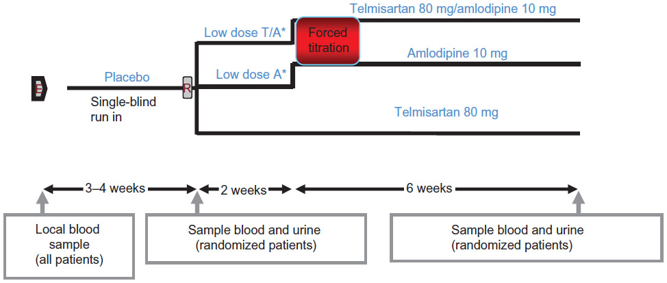Figure 1 Study design for this Phase III antihypertensive trial. Notes: *Low-dose telmisartan/amlodipine and low-dose amlodipine indicate that patients were randomized to SPC or to the amlodipine group and received 5 mg of amlodipine during the first 2 weeks. This is a double-blind study. After a 3–4-week single-blind run-in period, patients are randomized to 8 weeks of double-blind treatment in a 2:1:1 ratio. Abbreviations: A, amlodipine; T, telmisartan; SPC, single pill combination.

The protocol-specified testing procedure starts with the following primary hypotheses:

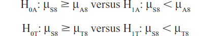
where μ_S8 is the mean change in SBP from baseline to week 8 in the SPC-treated group, and μ_A8 and μ_T8 are the respective changes in the amlodipine and telmisartan groups. The primary interest is to demonstrate that the SPC is superior to both of the component drugs after 8 weeks of treatment. Hence, both primary null hypotheses need to be rejected in order to demonstrate the efficacy of the SPC after 8 weeks of treatment and no adjustment for multiple testing is necessary. Because the objective is to show superiority, one-sided hypotheses are used. In Phase III, conventionally the two-sided α type I error is 0.05, and therefore, for these one-sided hypotheses tests, α=0.025 is used in testing each individual hypothesis.

If both of the above primary null hypotheses are rejected, the SPC can be claimed to be superior to both of the component drugs after 8 weeks of treatment and the primary objective of this study is achieved. However, if either one of the primary null hypotheses is not rejected, then further testing is stopped and the SPC cannot be claimed to be superior to both of the component drugs.

If the primary null hypotheses are rejected, then (as prespecified in the protocol) the following sets of key secondary hypotheses are tested:

where μ_Si is the mean change in SBP from baseline to week i in the SPC-treated group, μ_Ai and μ_Ti are the respective changes in the amlodipine and telmisartan groups; i = 6, 4, 2, and 1.

First, testing of the key secondary hypotheses at week 6 was planned. Again, if both respective null hypotheses can be rejected, superiority of the SPC after 6 weeks of treatment is demonstrated. This testing procedure continues to week 4, week 2, and week 1 in a stepwise sequence until either all the secondary null hypotheses (at week 6, week 4, week 2, and week 1) are all rejected (each at the one-tailed significance level of 0.025) or until at least one null hypothesis is not rejected. This follows a gatekeeping procedure and hence no alpha adjustment is necessary.

Statistical considerations

Longitudinal datasets are almost never complete and the analyst has to cope with missing data.¹ Traditionally, such datasets following patients over time were analyzed using last observation carry forward (LOCF) methodology in most of the Phase III clinical trials. The advantages of LOCF include: it implements the intent-to-treat principle; it satisfies the one-patient, one-vote approach; and it is easy to understand for nonstatisticians. Mallinckrodt et al² recommended using a mixed model with repeated measures (MMRM) for analysis of longitudinal clinical data. Siddiqui et al³ also argued that MMRM can be considered as an appropriate model of longitudinal data analysis in regulatory submissions. MMRM models are valid under missing at random assumptions.⁴ This Phase III antihypertensive study comparing the SPC of telmisartan and amlodipine with its monocomponents was conducted in 2008/2009 and the prespecified primary analytical model was MMRM in the protocol. Based on the study protocol, the proposed sensitivity analysis of the primary endpoint was LOCF.

The dataset for this study is interesting for three reasons: the timing of this study is around the time when the pharmaceutical industry and regulatory agencies are evolving statistical analysis from LOCF to MMRM; with an 8-week design and five time points for analysis, this study offers enough flexibility for consideration of a wide variety of statistical models; and the nature of this study requires analysis of each time point in a sequential fashion (week 8, then week 6, then week 4, then week 2, and finally week 1). Furthermore, clinical scientists have plenty of experience with antihypertensives, as blood pressure is a well established clinical endpoint, and it is a continuous measure (with normal distribution) where both LOCF and MMRM can readily be applied for data analysis. With over 800 patients recruited for this study, model convergence is not likely to be an issue. The results of the study are summarized in Figure 2.

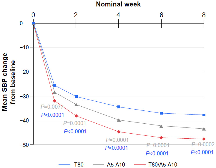Figure 2 Changes in SBP from baseline over 8 weeks. Notes: T80, telmisartan 80 mg; A5, amlodipine 5 mg; A10, amlodipine 10 mg. Abbreviation: SBP, systolic blood pressure.

The next section provides the primary analysis results based on MMRM, including the sensitivity analysis (LOCF) for the primary endpoint. This is followed by two sections describing alternative analyses. Finally a discussion is presented.

Primary analysis and sensitivity analyses

The prespecified primary analysis is based on an MMRM model, where the response is SBP change from baseline to week 8. Fixed effects include treatment, week, and treatment by week interaction. Baseline SBP is used as a fixed continuous covariate, and the baseline by week interaction is also included as a fixed effect. In this model, the patient is considered as a random effect, and an unstructured variance/covariance matrix is used for this random effect. For analyzing the primary endpoint, an MMRM model with high-dose amlodipine is used; this model included responses (SBP changes from baseline) at weeks 4, 6, and 8. For the analysis of response at weeks 1 and 2, a low-dose MMRM is used. In this low-dose MMRM, only responses at weeks 1 and 2 are included. Both models follow the specifications recommended in the 2008 Pharmaceutical Research and Manufacturers of America (PhRMA) position paper.²

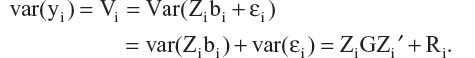
Linear mixed models have appeared extensively in the literature. We summarize some pertinent results below for convenience. Let i = 1, 2, … N index the number of subjects in a study, and let y_i be the column vector of observations made on the i-th subject. The dimensions of y_i, denoted by n_i, may be different across individuals, either by design or due to missing values. We consider a general linear mixed model of the form

where β is a column vector of fixed effects, X_i is a design (incidence) matrix relating the observations of the i-th subject to β, b_i is a column vector of random effects, Z_i is a design (incidence) matrix relating the observations of the i-th subject to b_i, and µ_i is a column vector of random errors. Assuming b_i and µ_i are independently distributed with zero mean and variance-covariance matrices, G and R_i, respectively, we have

and

The primary model includes five time points, ie, changes in SBP from baseline to weeks 1, 2, 4, 6, and 8. The variance-covariance matrix G was modeled as unstructured (UN). The SAS code of the primary model is given below:

proc mixed data=dta1235;

class ptno atr nomwk;

model syschg=atr nomwk atr*nomwk bsysse bsysse*nomwk/ddfm=kr s;

repeated nomwk/subject=ptno type=un r;

lsmeans atr*nomwk/pdiff cl;

run;

Note that two models were used in the clinical trial report for this study; one is the low-dose model, which includes responses up to weeks 1 and 2 and the other is a high-dose model that includes responses up to weeks 4, 6, and 8. In this paper, all these time points are included in a single model. The analytical results are summarized in Table 1.

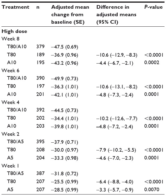Table 1 Summary of results from primary and secondary analysis using the PhRMA model Notes: T80, telmisartan 80 mg; A5, amlodipine 5 mg; A10, amlodipine 10 mg. Abbreviations: PhRMA, Pharmaceutical Research and Manufacturers of America; SE, standard error; CI, confidence interval.

Based on these results, it is clear that the SPC is significantly different from both of the component drugs at week 8 (P<0.0001 for the comparison of SPC against telmisartan and P=0.0002 for the SPC against amlodipine). Following the prespecified sequence of secondary endpoints, both null hypotheses (SPC compared with telmisartan and SPC compared with amlodipine) are rejected for week 8, week 6, week 4, week 2, and week 1: P-values for week 6 are <0.0001 and 0.0001; P-values for week 4 are <0.0001 and 0.0001; P-values for week 2 are <0.0001 and 0.0001; and finally, for week 1, the P-values are <0.0001 and 0.0070, respectively. Therefore, the primary analysis for the primary and secondary endpoints indicates that the SPC is superior to both of the component drugs across all time points (week 8, week 6, week 4, week 2 and week 1). In other words, the superiority of SPC against the individual component of either telmisartan or amlodipine started at week 1, and the separation continues throughout the entire 8 weeks.

For the primary endpoint (change in SBP at week 8) and the secondary endpoints, the sensitivity analysis is also performed, ie, LOCF up to weeks 8, 6, 4, 2, and 1. In these analyses, there are only two fixed effects, ie, the treatment effect and the continuous baseline covariate. Hence an analysis of covariance is performed to compare the treatment effect at weeks 8, 6, 4, 2, and 1 using the LOCF data. Note that when all of the post-baseline measurements are missing, the baseline is not carried forward.

From Table 2, the statistical significance at week 8 is detected when SPC is compared with telmisartan (P<0.0001) and with amlodipine (P<0.0001). These significant findings continue from week 8 down to week 6 (P-values are <0.0001 and 0.0002), week 4 (P-values are <0.0001 and 0.0002), week 2 (P-values are <0.0001 and 0.0002), and week 1 (P-values are <0.0001 and 0.0064). Results of these sensitivity analyses further support the primary analyses of both the primary and the secondary endpoints, indicating that SPC is superior to both of the component drugs at the primary time point (week 8), as well as the secondary time points (weeks 6, 4, 2, and 1) in treating patients with severe hypertension. Further, these comparisons are robust with respect to different data analysis models.

Table 2 Results of LOCF analysis Notes: T80, telmisartan 80 mg; A5, amlodipine 5 mg; A10, amlodipine 10 mg. Abbreviations: SE, standard error; LOCF, last observation carried forward; CI, confidence interval.

Alternative analysis: hybrid model considering time as continuous in random effect

One of the potential problems in implementing MMRM models is that when there are too many time points and without a large sample size, an unstructured covariance matrix may not be estimable. For example, in a study with a duration of 12 months designed with monthly visits (12 time points after baseline), the unstructured covariance matrix contains 78 (=12 * 13/2) parameters to be estimated. In practice, there can be missing data at various time points, and this may result in the MMRM algorithm not being able to converge. Typically under this situation, statisticians tend to choose a simpler covariance structure, such as compound symmetry or autoregressive of order 1, both of which require a smaller number of parameters to be estimated. However, these simpler covariance structures may not be justified by the data. When there are many time points and a compound symmetry covariance structure is assumed, it is questionable to assume that “the correlation between two neighboring time points is the same as the correlation between two time points that are very far apart.” In most of the therapeutic areas, such an assumption may not hold. Regarding the autoregressive covariance structure, although it may be appropriate in a design with equal time spacing, there can be problems under a general setting, in that correlations decay to zero fairly rapidly.

One proposal to balance the two problems, ie, not too many parameters in the covariance matrix and without very strong assumptions of correlation structure, is to assume a hybrid model. In this proposal, time is considered as discrete in the fixed effect, and then in modeling the random effect, time is considered as continuous. In such a hybrid model, the random effect can be expressed in terms of the covariance matrix G.

where b_1i is the intercept and b_2i is the slope estimate of the random effects, and g_mn is the variance (covariance) of the corresponding coefficients. Further, assuming ε_ijk is independent with variance σ², and b_i and ε_ijk are independent, then the variance of an observation is

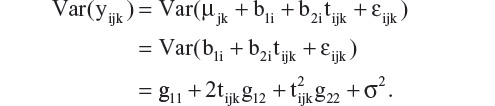
The covariance between two repeated observations within a subject is

It is clear that, under this model, both variance and covariance of the repeated measures are expressed as a function of time, t_ijk. As a consequence, this model accounts for heterogeneity of variances and covariances over time. Since t_ijk= 0 at baseline, Var(b_li) = g₁₁ is the between-subject variation in the mean response at baseline. The marginal variance of y_ijk at baseline is

In most of the clinical trial applications, the interest is on marginal means and their differences between treatment groups at a particular visit (eg, the treatment difference at week 8, μ_F8 − μ_T8 in the antihypertensive study comparing the SPC with its component drugs). The random effects are mainly used as a device to model the covariances among repeated measures within a subject.

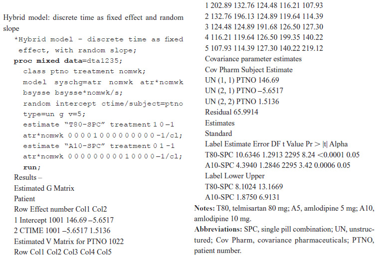
Under this setting, there are only four parameters that need to be estimated for the random effect: g₁₁, g₁₂, g₂₂, and the residual σ². This proposed alternative is more realistic and is practical because time is considered as continuous in the random effect, which reflects actual clinical practice. It is also invariant with respect to specification of time units. An analysis of the results using the proposed hybrid model is shown below. Details of the analysis, together with SAS code and SAS output, can be found in the Supplementary material.

In this analysis, a hybrid MMRM using discrete time as a fixed effect with a random slope (continuous time for the random effect) is fitted with the seated SBP observed post baseline. One advantage of this model is that the number of parameters associated with the random effect is reduced to only four, ie, g₁₁, g₁₂, g₂₂ and σ². In this example,

Based on these results, at a given time point t_ijk, the variance is Var , and for week 1, it is estimated as 146.69 + 2 (–5.6517) + 1.5136 + 65.9914 = 202.8916.

Covariance of time t_ijk and t_ijk’ can be obtained from .

For covariance at weeks 4 and 6 in the same subject, the estimate is 146.69 + 4 (−5.6517) + 6 (−5.6517) + (4) (6)(1.5136) = 126.4994.

The primary analysis for this antihypertensive trial is based on the PhRMA recommendation,² where the covariance matrix is modeled as unstructured. In this hybrid model, the covariance estimates are closer to the PhRMA model (used in the primary analysis) than to the compound symmetry (see Table 3). Under the compound symmetry model, three parameters are used for covariance estimates, while the hybrid model uses only one more. In the case where many time points are included in a trial, this hybrid model can be a reasonable alternative for consideration.

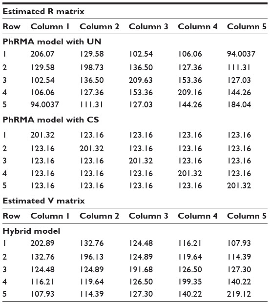Table 3 Covariance estimates obtained from the PhRMA model using unstructured and compound symmetry assumptions Abbreviations: CS, compound symmetry; UN, unstructured; PhRMA, Pharmaceutical Research and Manufacturers of America.

Interpretation of fixed effects is similar to that of the primary model (unstructured covariance matrix). Note that for the week 8 treatment effect, the SPC estimate is −47.5, the SPC-T80 difference is −10.6, and the SPC-A10 difference is −4.4. These estimates are almost identical (differences are in further digits after the decimal point) to the PhRMA model estimates. This alternative analysis using a hybrid model reached the same conclusion as the primary model. However, when comparing the t-values with the primary model (8.95 for T80-SPC and 3.71 for A10-SPC), the hybrid model seems to be less powerful.

For analysis of secondary endpoints, the hybrid model was applied to weeks 6 and 4 separately (although the SAS code in the supplement does not reflect this). Note that in the week 6 analysis, only data from weeks 1 to 6 were included, ie, week 8 data were excluded from the model. Similarly, in the week 4 hybrid model analysis, data obtained from time points after week 4 were excluded. The results are shown in Table 4 Note that in a simpler model with only two time points (eg, weeks 1 and 2), the covariance matrix obtained from the hybrid model employs the same number of parameters as those from unstructured covariance. Therefore, a separate hybrid model for weeks 2 and 1 was not performed. Results from weeks 6 and 4 of the hybrid model demonstrate statistical significance of the SPC against each of the component drugs both at weeks 6 and 4 (P-values for week 6 are <0.0001 and 0.0002; P-values for week 4 are <0.0001 and 0.0002). Results for weeks 2 and 1 can be obtained from the primary MMRM model, and are hence found in Table 1.

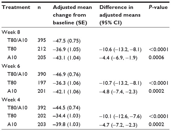Table 4 Analytical results from the hybrid mixed model with repeated measures Notes: T80, telmisartan 80 mg; A5, amlodipine 5 mg; A10, amlodipine 10 mg. Abbreviations: CI, confidence interval; SE, standard error.

The analysis results obtained from the hybrid model further support the conclusions from the primary MMRM model. This is consistent for the primary endpoint, and across all the secondary endpoints.

Alternative analysis: grouping method

In addition to typical LOCF analysis, MMRM, and the hybrid model, many other approaches can be applied to longitudinal data analysis. In the classification of missing data mechanisms, missing not at random (MNAR) can be further broken down into two subcategories, ie, nonignorable outcome-based dropout which depends directly on observed and unobserved outcome, and nonignorable random-coefficient-based dropout which depends indirectly on the outcomes through random coefficients.⁵ From a frequentist statistician’s perspective, as pointed out by Tipa et al,⁶ nonignorable random-coefficient-based dropout can be viewed as one type of nonignorable outcome-based dropout. In the setting of nonignorable random-coefficient-based dropout, Park et al⁷ proposed an asymptotically unbiased estimate of the overall treatment effect. Remarkably, one substantial advantage of their method lies in the fact that there is no requirement of any specified missing data model. Hence this advantage can be used to address some controversial issues that some other methods may have, such as misspecification of dropout model.

Additionally, more flexibility is available and generally appreciated, especially in clinical trials where a detailed statistical analysis plan must be fully specified before the treatment information is unblinded. Briefly, the idea of the grouping method is to group the patients into K subgroups depending on the total number of observed time points. Kong et al⁸ take this grouping approach and further broaden the treatment effects by using a saturated time effect model proposed by Wei and Shih.⁹ The resulting model provides an unbiased estimator for treatment effect at time tk. Here we will describe and then apply the method of Kong et al⁸ to the same antihypertension study. Without loss of generality, this approach readily applies to most of the longitudinal studies we commonly see. For better presentation of this approach, we first set up the notation of the model framework and then point out the difference from model 1. Let y_ij be the j-th component of y_i in (1), which denotes the efficacy endpoint of interest measured from the i-th patient at visit time t_j for i = 1, …, n and j = 1, …, K. The primary endpoint of this study, however, is the measurement at last visit t_k. Similar to model (1), y_ij is assumed to follows a linear mixed effects model,

for i = 1, …, n and j = 1, …, K. For the i-th patient, X_i is a p-dimensional vector which usually represents the baseline characteristics and treatment indicator; Z_i is a q-dimensional vector associated with the subject level random effect b_i, which is assumed to follow a multivariate normal distribution N_q(0, V). One exception is noted in the coefficient of X_i, denoted by β_j, which is no longer assumed to be constant over time. Compared with model 1, the major difference is that a random coefficient-based nonignorable dropout model is assumed, ie, the dropout probability for patient i is assumed to be an unspecified function of X_i and random coefficient b_i.

To estimate the treatment effect at time t_k, a least squares estimator based on the patients who remain in the study at time t_k can be written as

where R_K denotes the set of patients who remain in the study at time t_K. However, this estimator is not unbiased due to dropout at certain previous time t_j, for any j < K. In order to construct an unbiased estimator, Kong et al⁸ define a random variable, g_i, as the last visit time for the i-th patient. Based on g_i, the entire patient population can be partitioned into K subgroups, ie, {i:g_i = 1}∪{i:g_i = 2}∪…∪{i:g_i = K}, or compactly rewritten as In other words, each patient is classified based on their last available visit time.

Consequently, {i:g_i ≥ j} represents the subgroup of patients who remain in the study by time t_j. To simplify the presentation, denote S _j =Σ X_iX_i′, for j = 1,...,K. Then an unbiased estimator of is constructed as

This has been shown by Kong et al⁸ to be unbiased and also consistent for is β_k.

Next, we apply this model [2] to analyze this antihypertensive trial, and the results of comparing each component drug with the SPC are summarized in Table 5. R software version 2.15.1¹⁰ was used. Results for the primary and secondary endpoints are also summarized in Table 5. As seen in this table, analysis of the primary endpoint shows that at week 8, the treatment effect of the SPC subtracting the T80 group is −11.1, and the SPC subtracting the A10 group is −4.6. These estimates are close to the MMRM estimates (ie, SPC-T80 is −10.6 and SPC-A10 is −4.4). For this dataset, in order to compare the power of the Kong et al model with the primary model, we can check the test statistic, ie, the t-value or z-value in the output. As a result, the primary model yields 8.95 for SPC-T80, and 3.71 for SPC-A10, whereas the Kong et al model [2] provides 8.41 and 3.83, respectively. The power of model [2] seems to be comparable with the primary MMRM model in this antihypertensive trial. Comparisons at week 8 indicate that the benefit of SPC is statistically significant over each of the component drugs.

Table 5 Results from grouping method-based model Notes: T80, telmisartan 80 mg; A5, amlodipine 5 mg; A10, amlodipine 10 mg. Abbreviations: CI, confidence interval; SPC, single pill combination.

For analysis of secondary endpoints, the grouping method was applied to weeks 6, 4, and 2. Subsequent measurements beyond the specified visit have been excluded similarly, as described in the analysis using the hybrid model. For instance, in the week 6 analysis, only data from weeks 1 through 6 were included. Note that for week 1, the results obtained from either the primary analysis model or from LOCF should be sufficient. Therefore, week 1 analysis of the grouping method was not performed. The results in Table 5 from weeks 6, 4, and 2 are highly statistically significant, as similarly established in the primary analysis as well as the one using the hybrid model. This reconfirms the superiority of SPC against each of its components.

Discussion

In longitudinal clinical trials, missing data caused by patient dropout often makes it difficult to draw definitive conclusions. In order to minimize this problem in Phase III studies, many important considerations are implemented in the design and trial conduct stage. Once the study is completed and the database is locked, there is not much that can be done to bring the missing data back into the trial. The primary statistical analyses will be performed on the locked database to help formulate the study conclusion. At this stage, in order to demonstrate the robustness of the conclusion, various sensitivity analyses would be performed to see if the primary conclusion can be affected by missing data.

A Phase III antihypertensive clinical trial is introduced in this paper. The objective of this trial is to demonstrate superiority of the treatment effect from an SPC comparing against each component drug. The SPC is a combination of telmisartan 80 mg plus amlodipine 10 mg and the trial was designed to demonstrate that the SPC is superior to both telmisartan and amlodipine. In this 8-week study, the primary endpoint is change from baseline in SBP up to week 8. Secondary endpoints are changes in SBP from baseline up to weeks 6, 4, 2, and 1.

In dealing with missing data, in the past the most frequently used method in the primary statistical analysis of a longitudinal trial was LOCF. However, since publication of the paper by Mallinckrodt et al² in 2008, many clinical statisticians have used MMRM to handle the missing data problem. In analyzing the SBP data from this Phase III antihypertensive trial, we prespecified MMRM as the primary model, together with LOCF for sensitivity analysis. The primary analysis is based on two prespecified models: the high-dose model that uses responses at weeks 4, 6, and 8, where the week 8 response is the primary time point, and the low-dose model that uses only weeks 1 and 2 data as responses. In both models, fixed effects include treatment, week, and treatment by week interaction. Baseline SBP is used as a fixed continuous covariate, and the baseline by week interaction is included as a fixed effect. Random effect includes patient effect and residual. The patient effect over time is modeled with an unstructured variance/covariance matrix.

In this paper, two alternative analytical methods are introduced, ie, a hybrid MMRM using time as a continuous variable in the random effect (while maintaining time as a discrete variable in the fixed effect) and a grouping method. Statistical analyses were applied to this set of SBP data including the prespecified MMRM, the LOCF sensitivity analyses, as well as these alternative analyses. All analytical results demonstrate a consistent conclusion that the telmisartan plus amlodipine SPC is significantly superior to both of the monotherapies in patients with severe hypertension starting from week 1 post randomization, and throughout the entire 8 weeks of double-blind treatment. For this set of SBP data, the clinical conclusion is robust, regardless of the model choices used for statistical analysis.

Acknowledgment

The authors express their sincere appreciation to the team members who participated in and contributed to this clinical trial.

Disclosure

The authors report no conflicts of interest in this work.

---

References

1.	Little RJA, D’Agostino R, Dickersin K, et al. The Prevention and Treatment of Missing Data in Clinical Trials. Washington, DC: The National Academies Press; 2010.
2.	Mallinckrodt CH, Lane PW, Schnell D, Peng Y, Mancuso JP. Recommendations for the primary analysis of continuous endpoints in longitudinal clinical trials. Drug Inf J. 2008;7:303–319.
3.	Siddiqui O, Hung HM, O’Neill R. MMRM vs LOCF: a comprehensive comparison based on simulation study and 25 NDA datasets. J Biopharm Stat. 2009;19:227–246.
4.	Little RJA, Rubin D. Statistical Analysis of Missing Data. New York, NY: John Wiley & Son Inc; 2002.
5.	Little RJ. Modeling the dropout mechanism in repeated-measure studies. J Am Stat Assoc. 1995;90:1112–1121.
6.	Tipa M, Murphy S, McLaughlin D. Ignorable dropout in longitudinal studies. 1996. Available from: http://www.amstat.org/sections/srms/Proceedings/papers/1996_118.pdf. Accessed October 22, 2013.
7.	Park S, Palta M, Shao J, Shen L. Bias adjustment in analyzing longitudinal data with informative missingness. Stat Med. 2002;21:277–291.
8.	Kong F, Chen Y, Jin K. A bias correction in testing treatment efficacy under informative dropout in clinical trials. J Biopharm Stat. 2009;19: 980–1000.
9.	Wei L, Shih WJ. Partial imputation approach to analysis of repeated measurements with dependent drop-outs. Stat Med. 2001;20:1197–1214.
10.	The R Project for Statistical Computing. A language and environment for statistical computing. 2012. Available from: http://www.R-project.org. Accessed October 22, 2013.

---

Supplementary material