Local in Time Statistics for detecting weak gene expression signals in blood – illustrated for prediction of metastases in breast cancer in the NOWAC Post-genome Cohort

Background

Breast cancer is the most common invasive cancer in women worldwide with an estimated 1.7 million new cases in 2012, representing 25% of all cancers in women.¹ The incidence of breast cancer is expected to increase substantially, especially in developing countries due to changing lifestyle.¹ Breast cancer has a relatively high survival rate, up till the point where a metastasis is present, at which time the survival rate drops dramatically. One hundred years ago, the survival rate of women with metastatic cancer was only 5% after 5 years,² while today it is 85%, depending on the stage (stage II 89%, stage III 76%, and stage IV 27%).³ Still the major challenge in breast cancer treatment is the diagnosis and subsequent treatment of metastases. Although significantly improved, the majority of cancer deaths are due to metastases, not due to the primary tumor.^4,5

No unifying theory exists for the human carcinogenesis, although many proposals exist.⁶ To date, most mechanistic or pathway-level analyses have been experimental in vitro or animal studies. With the increasing knowledge about human carcinogenesis in tumor tissues or in blood at time of diagnosis, some thought-provoking facts about the validity of using animal models to study carcinogenesis in humans have been brought up. First, the biology of mice and humans is comparatively different,⁷ and a Nature editorial⁸ advocated the need for human functional studies. Similarly, the translational value of mouse models in oncology drug development was recently questioned.⁹ While cancer can be developed in mice quite easily, these models do not necessarily apply to humans.¹⁰ An alternative approach is using functional transcriptomics, including epigenetic and transcriptomic biomarkers to jointly assess both the exposure and outcomes. This “meet in the middle approach”¹¹, however, does not take into account the time dependency of the carcinogenic process.

The recent focus on the metastatic process^12–14 has revealed some crucial questions: what is the best biological model for the metastatic process and how to develop prediction methods for translation to clinical tests?

Contrary to classical epidemiology focusing on risk estimation, the processual approach does not use time for estimating relative risk of disease given certain exposures. Rather the processual approach within a systems epidemiology framework¹⁵ explores human carcinogenesis through the analysis of functional genomics. The statistical quantity of interest is the distribution of the differences in log₂ gene expression in blood between breast cancer cases and healthy controls, and how this quantity is associated with the time from blood sampling to cancer diagnosis. Since there is a priori no knowledge of the time-dependent distributions of gene expression profiles related to the metastatic process, we present a new statistical method together with real data as a proof of concept. Few prospective studies have been designed for longitudinal analyses of functional genomics related to the processes of carcinogenesis and metastasis.

We hypothesize that cancer cells spreading through the blood or the lymphatic system elicit an immunological response that should be measurable as dynamic gene expression profiles in cells of the immune system, long before the metastasis is clinically detectable. Preserving the gene expression signals in blood requires specific care in sample collection and storage, and in the Norwegian Women and Cancer (NOWAC) Post-genome Cohort adequately buffered blood samples were collected from healthy women.

In a previous methodological study, time was categorized in three periods.¹⁶ In the approach presented herein, we are able to better identify the points in time relative to cancer diagnosis where changes in gene expression occur. Also previously, the same dataset has been analyzed focusing on weak signals from a large number of genes.¹⁶ The main aim of this paper is to explore the dynamic, time-dependent mechanisms of the metastatic processes using blood transcriptomics and including time in a continuous manner. For achieving this goal, we will develop new statistical methods based on statistics that are local in time, where the objective is to be able to identify small changes that vary slowly in time and/or between strata, by using a large number of genes in each hypothesis test and predictor. This paper presents as an example longitudinal analyses of transcriptomic data using the processual approach¹⁷ within the NOWAC Post-genome Cohort.

Methods

We describe a new statistical method, Local in Time Statistics (LITS), for a processual analysis of functional genomics in blood. More precisely, this is a method for analyzing gene expression profiles in blood samples collected before diagnosis of some diseases, eg, breast cancer, where the dataset consists of case-control pairs and the case is diagnosed with the disease, while the control is healthy. The cases should belong to one of two strata, eg, cancers with and without metastases. The data for a pair that are used by the method are the difference in log₂ gene expression between the case and the control. The gene expression profiles that are measured represent an aggregate of the transcriptional activity of all the blood cells at the time of blood collection.

The method will be used for examining whether the gene expression profile varies with time from blood sampling to diagnosis, between cases and controls, or between the two strata. Lastly, the LITS method will be used for predicting the stratum for a case, eg, whether a case has breast cancer with or without metastases. Details about the statistical methods and the available dataset are given below.

As mentioned in the “Background” section, we categorized time in three periods in a previous methodological study,¹⁶ and the new method presented in the study is a further development of this method that is more continuous in time and thereby is better able to identify the points in time relative to diagnosis where changes in gene expression occur. The authors are not aware of other non-parametric, continuous in time approaches suitable for analyzing the kind of data described above.

Statistical methods

As a central part of the statistical methodology is to examine how gene expression varies with time to diagnosis, we will divide the time before diagnosis into time periods. The time periods will be overlapping as we will use a moving window in time when defining the periods. The lengths of the time periods are chosen such that we obtain as short time periods as possible (as the distribution of the gene expressions may vary with time from blood sampling to diagnosis), but at the same time such that there are as many case-control pairs as possible within each time period (to obtain as good estimates as possible for each time period). There is a trade-off between these two wishes. We use the following procedure when defining the time periods for datasets that consist of one or two strata, eg, two strata consisting of cases with cancers with and without metastases: Let T be the number of case-control pairs in the stratum with the highest number of such pairs. Let t₁ ≤ t₂ ≤ … ≤ t_T be the time to diagnosis for these T pairs. The T – S + 1 time periods are then defined as the intervals [t₁, t_S] [t₁, t_S+₁], … ,[t_T–S+₁, t_T], where S is chosen such that we obtain short time periods with many case-control pairs from each stratum.

Let X_g,c be the difference in log₂ gene expression for case-control pair c, c = 1, …, M, where M is the number of case-control pairs, and gene g, g = 1, …, N, where N is the number of genes. Let μ_g,s,t and s_g,s,t be the expectation and standard deviation of X_g,c, respectively, where s is one of two strata, eg, strata consisting of cases with cancers with and without metastases, and t is the time to diagnosis for X_g,c. If the distribution of X_g,c does not vary in time or between strata, the expectation and variance of X_g,c are independent of time and stratum, ie, μ_g,s,t = μ_g and s_g,s,t = s_g for all strata s and time before diagnosis t. Also, if there is no difference between cases and controls, the expectation of X_g,c is zero, ie μ_g,s,t =0.

Hypothesis tests for finding signal in the data

For examining whether there are differences between cases and controls, between strata or in time, we will test different hypotheses. For each hypothesis, the test statistic will be based on either expectation or standard deviation or both. The null distribution of the statistic will be estimated by randomizing the data, and we compute p-values by comparing the statistic for the data to the estimated null distribution. This will be described in more detail in the next section.

Let m_p,g be the sample mean and s_p,g be the sample standard deviations for the differences in log₂ gene expressions for gene g in time period p. Let m_p,g,1 (m_p,g,0) be the sample mean and s_p,g,1 (s_p,g,0) be the sample standard deviations for the differences in log₂ gene expression for gene g in time period p for stratum 1 (0).

We define the statistics s_p,(g), m_p,(g), and w_p,(g) from these sample means and standard deviations as follows:

• s_p,(g)=s_p,g’, where s_p,g’ has rank g when the s_p,g’s for period p are sorted in increasing order. Rank 1 corresponds to the smallest of the s_p,g’s for period p.
• m_p,(g)=|m_p,g′|, where |m_p,g′| has rank g when the |m_p,g|’s for period p are sorted in decreasing order. Rank 1 corresponds to the largest of the |m_p,g|’s for period p.
• Let 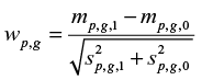be the weight for gene g in time period p, ie, a measure of the difference between the two strata. w_p,(g)=|w_p,g′| where |w_p,g′| has rank g when the |w_p,g|’s for period p are sorted in decreasing order. Rank 1 corresponds to the largest of the |w_p,g|’s for period p.

These three statistics are used for testing the three null hypotheses described below. Previously, we proposed and tested the variables s_p,(g) and w_p,(g).¹⁸ The strength of the hypothesis tests depends on the selected rank. Different ranks were examined. We also proposed and tested the statistic m_p,(g) on synthetic data.¹⁹ If there is a difference in average value of X_g,c between the strata for some of the genes, but we do not know which genes, and the difference is normally distributed, then the statistical tests are strongest for a small rank. If the distribution has heavier tails than the normal distribution, we should focus on the few genes with strongest signal, and if the distribution has less heavy tail, for example, a constant difference in the average value, then the statistical test is strongest for a larger rank, often larger than (closer to) the number of genes with a difference in average value between the strata.^18,19

H0-case-ctrl

The expectation of X_g,c is zero. This means that there is no difference between the expectations of the log₂ gene expression values for the cases and controls. If the null hypothesis is false, the expectation will be different from zero for some periods and genes. We test the hypothesis by using the statistic m_p,(g).

H0-time

The distribution of X_g,c is not associated with the time to diagnosis. This means that the expectation and standard deviation of X_g,c are the same in all time periods. If the null hypothesis is false, the standard deviation for some periods will be lower than the standard deviations for the entire time period for some genes. Also, the absolute value of the expectation for some periods will be higher than the absolute value of the expectation for the entire time period for some genes. We test the hypothesis first by using the statistic s_p,(g), and then by using the statistic m_p,(g).

H0-node

The expectation of X_g,c is not associated with stratum (eg, metastases or not metastases). This means that μ_g,1,t=μ_g,0,t, ie, the expectations for the two strata are equal for all genes g and time to diagnosis t. If the null hypothesis is false, the difference in expectation will be different from zero for some periods and genes. We test the hypothesis by using the statistic w_p,(g).

We will reject the H0-case-ctrl hypothesis if the hypothesis m_p,(g) >0 is rejected for at least one time period p and rank g, where g belongs to a subset of the N ranks. In practice, we have chosen to let the subset of ranks consist of ranks between approximately 1% and 25% of the number of genes, so that the subset contains both relatively low and high ranks. This means that H0-case-ctrl is rejected based on a very large number of hypotheses, which are also highly positively correlated. We take this into account by using the Benjamin-Hochberg procedure for controlling the false discovery rate (FDR).²⁰ The approaches for rejecting the H0-time and H0-node hypotheses are similar. Besides rejecting the three null hypotheses, the hypothesis tests for the statistics for each time period and rank will be used for illustrating how the p-values are associated with the time to diagnosis.

Randomization for estimating null distributions and p-values

We compute p-values by estimating the null distribution for the statistic of the hypothesis test by randomizing the data, ie, interchanging covariates (time to diagnosis, case/control, etc.) between the patients. In the randomization, we preserve critical properties of the genes (level of expression, complex correlation between genes, etc.) and randomize only what is connected to the changes in time, stratum, or case/control status. This randomization defines the null distribution for the test statistic that is used when finding the p-value. We randomize the data either by randomizing the case and control in each case-control pair (H0-case-ctrl), by randomizing the case-control pairs between the periods (H0-time), or by randomizing between the two strata within the time period (H0-node). We explain each randomization strategy in more detail in the following sections:

Randomization strategy for H0-case-ctrl

The null distributions of the statistics are estimated by randomizing the case and control in each case-control pair. In practice, this is done by keeping the absolute value of all log₂ gene expression differences, but by simulating their signs.

Randomization strategy for H0-time

The null distributions of the statistics are estimated by randomizing the case-control pairs between the periods.

Randomization strategy for H0-node

The null distribution of the statistic is estimated by randomizing between the two strata within the time period. Note that we compute w_p,(g) only if there are at least three case-control pairs in period p for each stratum. If this is not the case, we set the p-value to 1 for this period for all genes.

Note that all three randomization strategies maintain the correlation structure between the genes for each case-control pair. Also note that each randomization of the data leads to a different ordering of the genes when the genes are ordered according to the statistic of the hypothesis test. The p-value of the test was set to , where N_s is the total number of randomizations and K is the number of randomizations out of N_s with a more extreme statistic than the statistic for the real data. In the results presented we used N_s =1000.

Predicting stratum

The weights w_p,(g) can be estimated for each rank g from data in period p for a training dataset. The stratum of the case of a new case-control pair, ie, a case-control pair that does not belong to the training set, can then be predicted based on the score

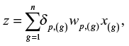
where x_(g) is the difference in log₂ gene expressions of the new case-control pair and d_p,(g) is 1 if the weight w_p,g′ is positive and −1 otherwise, where |w_p,g′|= w_p,(g). The n genes with highest absolute value of the weights are used for computing the score, where n is a number less than or equal to the number of genes, N. Large values of z indicate that the new case belongs to stratum 1. If z > c for some arbitrary threshold c, we conclude that the new case belongs to stratum 1, otherwise we conclude that the new case belongs to stratum 0. We may set c=0 if it is not more important to avoid false classification in one stratum relative to the other and if

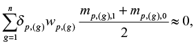
where m_p,(g),1 and m_p,(g),0 are the sample means that are used when computing w_p,(g). Increasing (decreasing) c results in fewer false positives (negatives) at the cost of more false negatives (positives).

When predicting the stratum of the cases in the same dataset as we use for estimating the weights w_p,(g), we use the leave one out approach, ie, when predicting the stratum of the case j we use weights w_p,(g) that have been estimated using the training dataset after case-control pair j has been excluded. The reason why we chose to use the leave one out approach is that the dataset is too small to be divided into a training and validation set. The strength of the prediction rule should be determined from data that are not used for estimating the prediction rule.

Example from the NOWAC Post-genome Cohort study

The NOWAC study is a nation-wide population-based cancer study that was initiated in 1991.²¹ The biobank of the Post-genome Cohort has been described previously in detail.²² Briefly, the invited women were randomly drawn from the Central Person Register by Statistics Norway, and non-respondents received one or two reminders. Women who agreed to give a blood sample were divided at random into batches of 500, and received a 2-page questionnaire and the PAXgene blood RNA collection kit (PreAnalytiX GmbH, Hombrechtikon, Switzerland), which contains an mRNA-stabilizing buffer. Blood sampling was performed at the family doctor’s office, and blood samples were returned via mail to the study center. One reminder was sent after 4–6 weeks. A total of 48,692 blood samples were collected in the years 2003-2006, corresponding to 72.2% of the invited women.

By linkage to the Cancer Registry of Norway, a total of 637 cases of invasive breast cancer in the Post-genome Cohort were reported for the years 2003–2010. For each case of breast cancer, a control from the same batch was assigned, matched by time of blood sampling and year of birth without replacement. After removing technical outliers, and ineligible cases including women with distant metastases (stage IV) and case-control pairs in which controls were diagnosed with cancer within 2 years of blood sampling, the study consisted of 546 in situ and breast cancer case-control pairs. Information on lymph node status at breast cancer diagnosis was based on the pathological tumor-node-metastasis staging information included in the Cancer Registry of Norway. Detection categories were also obtained from the screening database kept by the National Breast Cancer Screening Program²³ hosted by the Cancer Registry of Norway.

Each woman gave one blood sample, and case-control pairs were ranked according to the time interval between blood sampling and cancer diagnosis. Collectively, the case-control pairs provide information on blood gene expression up to 8 years before diagnosis.

Study design

All statistical analyses were performed separately for the screening and clinical group. The screening group consists of cases diagnosed with cancer during a screening visit or within 2 years of the last screening, ie, interval cancers, while the clinical group consists of cases with cancers that were diagnosed clinically and that did not attend screening or had not attended screening for the last 2 years. Each case belongs to one of the two following strata: with metastases or without metastases.

Ethical issues

The NOWAC study including the Post-genome Cohort was approved by the Norwegian Data Inspectorate and recommended by the Regional Ethical Committee (REK). The linkages of the NOWAC database to national registries such as the Cancer Registry of Norway and registries on death and emigration have also been approved, and the women were informed about these linkages. Furthermore, the collection and storing of human biological material were approved by the REK in accordance with the Norwegian Health Research Act. The women gave informed consent explicitly for gene expression analyses in the blood samples.

Laboratory procedures

All laboratory work and microarray services were provided by the Genomics Core Facility, Norwegian University of Science and Technology, Trondheim, Norway. To control for technical variability such as different batches of reagents and kits, day-to-day variations, microarray production batches, and effects related to different laboratory operators, each case-control pair was kept together throughout all extraction, amplification, and hybridization procedures. Total RNA was extracted using the PAXgene Blood miRNA Isolation kit (PreAnalytiX/Qiagen, Hilden, Germany) according to the manufacturer’s instructions. RNA quality and integrity were assessed using the NanoDrop ND 8000 spectrophotometer (ThermoFisher Scientific, Wilmington, DE, USA) and Agilent Bioanalyzer (Agilent Technologies, Palo Alto, CA, USA), respectively. Total RNA (300 ng) was amplified and labeled using the Illumina TotalPrep-96 RNA Amplification Kit (Ambion Inc., Austin, TX, USA). All case-control pairs were run on either the Illumina HumanWG-6 version 3 expression bead chip or on the Illumina HumanHT-12 version 4 bead chip. Outliers were excluded after visual examination of dendrograms, principal component analysis plots, and density plots. Individuals who were considered borderline outliers were excluded if their laboratory quality measures were below given thresholds: Bioanalyzer RNA integrity number (RIN)<7, NanoDrop 268/280 ratio<2, and 260/230 ratio<1.7, and NanoDrop RNA concentration between 50-500 ng/microliter.

Preprocessing of microarray data

The dataset was preprocessed as previously described.²⁴ The dataset, which consisted of 546 case-control pairs and 30,046 probes, was background corrected using negative control probes, log₂ transformed using a variance stabilizing technique,²⁵ and quantile normalized. Data from the two Illumina chips (HumanWG-6 v3 and HumanHT-12 v4) were combined on identical nucleotide universal identifiers.²⁶ We retained probes present in at least 70% of the individuals. If a gene was represented with more than one probe, the average expression of the probes was used as expression value for the gene, resulting in a dataset with 8155 genes. The probes were translated to genes using the lumiHumanIDMapping.²⁷ Finally, the differences of the log₂ gene expression levels for each case-control pair were computed and used in the statistical analyses. We then excluded data for the 79 case-control pairs where the case was diagnosed with in situ cancer so that the final, preprocessed dataset included 467 case-control pairs.

The data are from three different runs and there are batch effects between runs. The obtained estimates for the batch effects were more different than expected by chance. We demonstrated this by randomizing data between the batches/runs. We therefore estimated these batch effects (see Supplementary material) and included the estimates in the methods that were used for analyzing the data. Note that some batch effects disappeared when we computed differences in log₂ gene expression between cases and controls, while other batch effects did not disappear. See Supplementary material for more details.

Results

Details about the dataset used in the analyses, like the number of case-control pairs in each stratum and the distribution of the case-controls pairs in time, are given in Tables 1 and 2. The data used in all analyses are the differences in log₂ gene expression between cases and controls. Figure 1 gives an overview of datasets and strata that are included in the different statistical analyses.

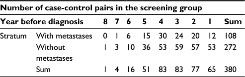Table 1 Number of case-control pairs with gene expression data Xg,p in each stratum and year before diagnosis in the screening group

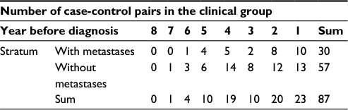Table 2 Number of case-control pairs with gene expression data Xg,p in each stratum and year before diagnosis in the clinical group

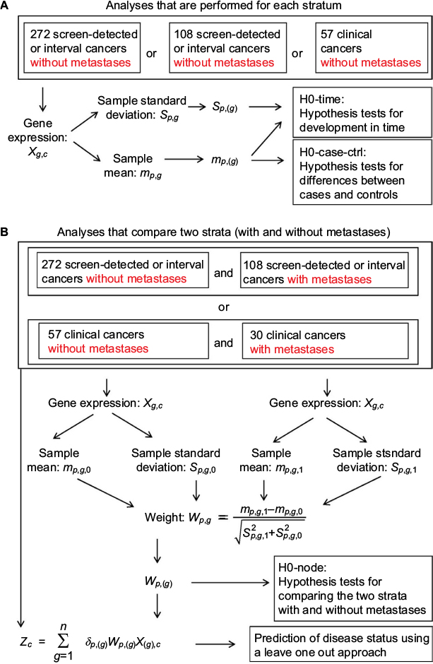Figure 1 Overview of hypothesis tests, prediction methods, variables, and strata. Notes: Illustration of the association between the data Xg,p, the different hypothesis tests, the prediction methods, the variables used in these tests and methods, and the strata.

Table 3 illustrates the biological differences between breast cancer diagnosed as part of participation in the screening program or diagnosed outside the screening as part of clinical practice. In the screening program, there is a significant association between the metastatic status and size of the tumor, which is not found for clinical cases.

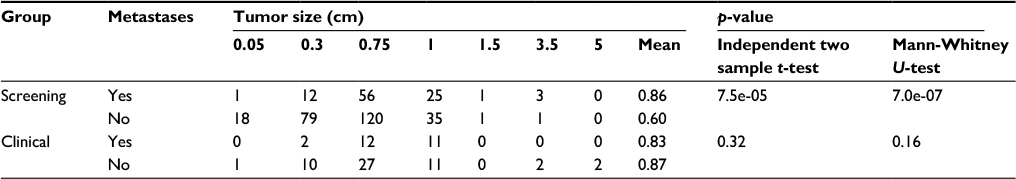Table 3 Association between tumor size and metastases Notes: p-values are obtained using an independent two sample t-test (testing if averages are equal) and a Mann-Whitney U-test (testing if it is equally likely that the tumor size of a case with metastases is less than or greater than the tumor size of a case without metastases).

Dividing into time periods

We divided the time before diagnosis into overlapping time periods using a moving window and the approach is described in the “Methods” section. Time periods defined for the clinical group contain 25 cases without metastases and 9–17 with metastases. The lengths of the time periods are 605–971 days, except for the four periods that include the case-control pairs in year 6 and 7 before diagnosis. Time periods defined for the screening group contain 50 cases without metastases and 11–32 with metastases. The lengths of the time periods are 256–796 days, except for the period that includes the case-control pair in year 8 before diagnosis. In analyses that only include cases with metastases from the screening group, we selected time periods that contain 50 cases with metastases. Note that we did not perform analyses for cases with metastases from the clinical group as this dataset was too small. When estimating s_p,(g), we used time periods that included at least 35 cases without metastases as more data are needed to obtain reliable estimates of the standard deviation than the mean.

In the next section, we compare the period closest to and furthest from time of diagnosis. For the screening group, the time period closest to diagnosis is 1–338 days before diagnosis (year 1), while the time period furthest from diagnosis is 1470–2736 days before diagnosis (five months of year 5, year 6, year 7, six months of year 8). For the clinical group, the time period closest to diagnosis is 1–612 days before diagnosis (year 1, eight months of year 2), while the time period furthest from diagnosis is 1090–2274 days before diagnosis (year 4, year 5, year 6, three months of year 7).

Hypothesis tests and multiple testing

When testing the null hypotheses H0-time, H0-case-ctrl, and H0-node, we included statistics for all time periods and genes with ranks between 50 and 2000, ie, between approximately 1% and 25 % of the number of genes, in total approximately 45,000–450,000 tests for each null hypothesis. When testing whether s_p,(g) was smaller than expected, more than 25% of the tests both for the screening and for the clinical group were rejected at the 5% FDR level. For the screening group and the tests m_p,(g) > 0 (H0-time), m_p,(g) > 0 (H0-case-ctrl), and w_p,(g) > 0, we rejected 1%, 2.4%, and 4.5% of the tests at the 10%, 12%, and 20% FDR level, respectively. For the clinical group, we obtained no significant results for these three groups of tests (FDR 20%). The reason for this may be that the clinical dataset is too small.

Based on these results, we can reject all the three null hypotheses H0-case-ctrl, H0-time, and H0-node, and conclude that there are differences between cases and controls, that these differences are associated with time to diagnosis, and that there are differences between the two strata with and without metastases.

Comparing the period closest to and furthest from time of diagnosis

Figure 2 shows plots of the statistics s_p,(g) and m_p,(g), while Figure 3A shows plots of the statistic w_p,(g). In these plots, we focus on the difference between data close to and far from diagnosis. In Figure 2B, we show results only for data without metastases, instead of both with and without metastases as in Figure 2A, since there are so few case-control pairs with metastases in the clinical group.

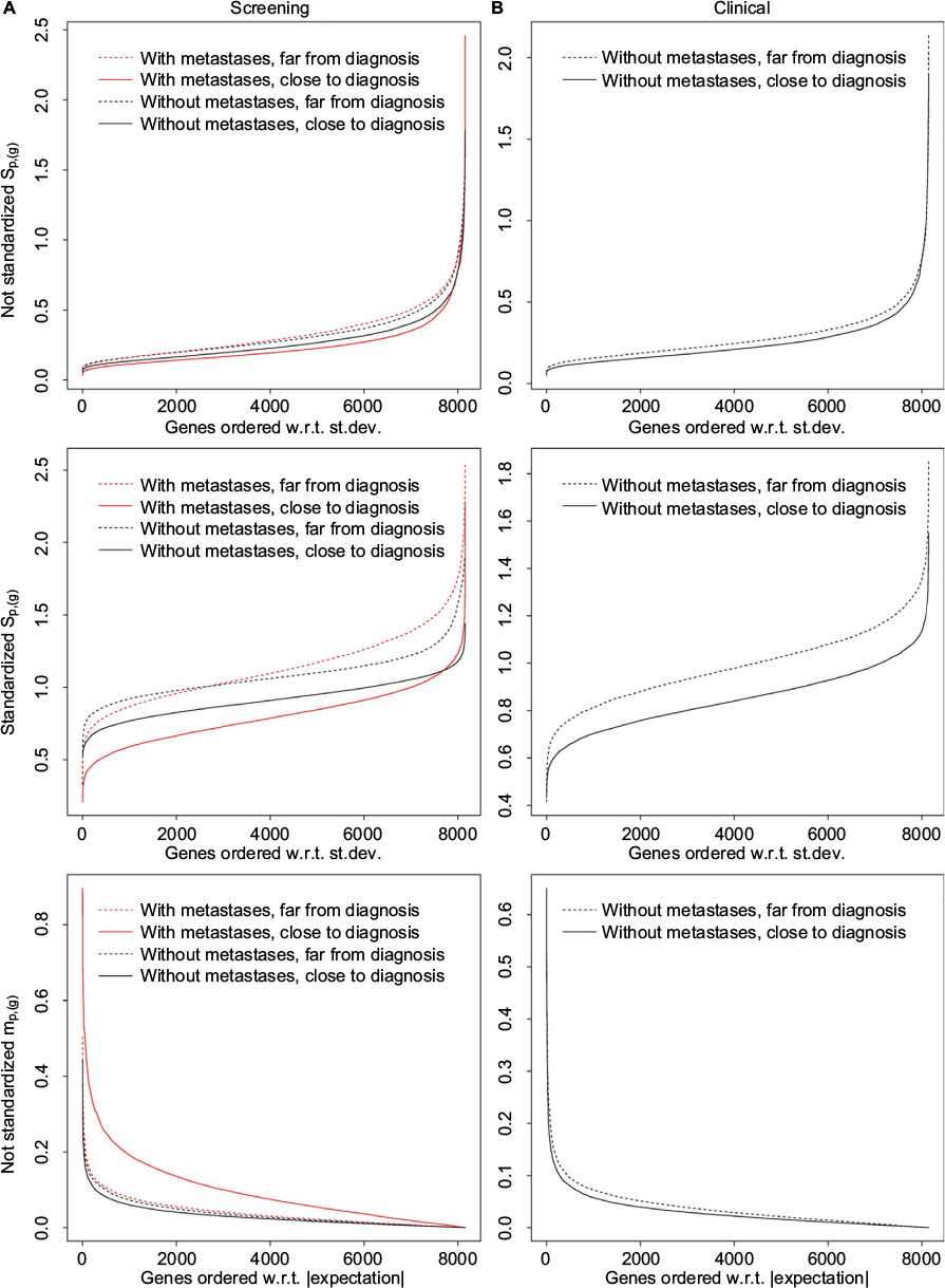Figure 2 The statistics sp,(g) and mp,(g). Notes: Plots are shown for not standardized data for sp,(g) and mp,(g), and also for standardized data for sp,(g). Curves are shown for the data in the period closest to and furthest from diagnosis. (A) Data from the screening group. (B) Data from the clinical group. Abbreviations: st.dev., standard deviation; w.r.t, with respect to.

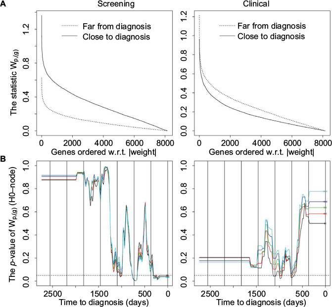Figure 3 The statistic wp,(g) and hypothesis H0-node. Notes: Plot of statistic (A) and plot of p-values against time (B) for the statistic wp,(g) for the screening (left panel) and clinical group (right panel). (A) Plot of the statistic wp,(g) where the two periods contain 50 (screening) or 25 (clinical) case-control pairs where the case is without metastases. (B) Plot of p-values against time for the statistic wp,(g) (H0-node). In each plot, there is one curve for genes with order 50 (black), 200 (red), 500 (green), 1000 (blue), and 2000 (light blue), respectively. p-value for time point t is equal to the p-value for the time period with middle point closest to t (after the p-values have been smoothed using a median filter with window size 99). The resulting curve is then smoothed using a mean filter with a window size of 1 month. The dotted horizontal line indicates a 0.05 level of significance, while the long vertical lines indicate the years before diagnosis. Abbreviation: w.r.t, with respect to.

We show results for the statistic s_p,(g) for two variants of the dataset, one where we have standardized the data, ie, X_p,c, to expectation zero and standard deviation one for each gene, and one without standardizing the data. We observe that the shapes of the curves for the two variants of the datasets are quite different. In the plot with not standardized data, there are many small and few large standard deviations, while the standard deviations, as expected, are around 1 for the standardized data. Note that for both the screening and the clinical groups, we also observe that s_p,(g) is larger far from diagnosis (H0-time). For the screening group, s_p,(g) is smaller with metastases close to diagnosis (H0-time). The difference between the two types of cases (with and without metastases) also implies a difference between cases and controls (H0-case-ctrl). As results for other statistics than s_p,(g) are not much influenced by standardizing the data, all results for these statistics are shown for data that are not standardized. For the same reason, results including the statistics s_p,(g), m_p,(g), and w_p,(g) presented later in this paper will also be based on data that are not standardized.

From the plots in Figure 2 that are based on the sample mean m_p,(g), we observe that for the screening group, the statistic is largest for the case with metastases and close to diagnosis (H0-time). For the clinical group, the statistic is quite similar for the two periods close to and far from diagnosis.

Figure 3A shows results for the statistic w_p,(g) that measures the difference between the log₂ gene expression of the cases with and without metastases relative to their standard deviations. For the screening group, the statistic w_p,(g) is largest close to diagnosis, while for the clinical group the difference is smaller and in the opposite direction, ie, largest far from diagnosis (H0-node). The difference in the screening group between without and with metastases may be due to the difference in expectation, as shown in Figure 2.

Development in time before diagnosis

Previously, we concluded that we can reject all the null hypotheses, H0-case-ctrl, H0-time, and H0-node. For each of these null hypotheses, we tested different hypotheses for the different time periods using a moving window. Figure 3B and Figure 4 show how the p-values of these tests vary with time. Note that Figure 4 includes results for the stratum without metastases.

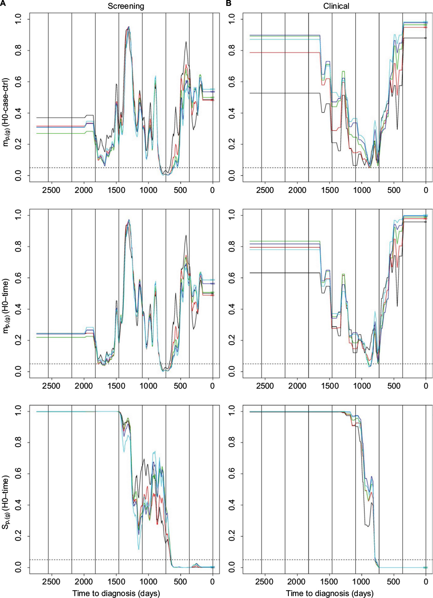Figure 4 Hypotheses H0-case-ctrl and H0-time. Notes: Plots of p-values against time for the hypotheses H0-case-ctrl and H0-time where the datasets with cases without metastases are used. (A) Results for data from the screening group. (B) Results for data from the clinical group. In each plot, there is one curve for genes with order 50 (black), 200 (red), 500 (green), 1000 (blue), and 2000 (light blue), respectively. p-value for time point t is equal to the p-value for the time period with middle point closest to t (after the p-values have been smoothed using a median filter with window size 99). The resulting curve is then smoothed using a mean filter with a window size of 1 month. The dotted horizontal line indicates a 0.05 level of significance, while the long vertical lines indicate the years before diagnosis.

In the upper panel of Figure 4, we observe that there are significantly high values for the sample mean m_p,(g) (H0-case-ctrl, randomizing between the case and control) around 2 years before diagnosis for the screening group without metastases, and almost significant around year 3 before diagnosis for the clinical group without metastases. No significant results were obtained for the screening group with metastases for m_p,(g), neither for H0-case-ctrl nor for H0-time.²⁴ As the group without metastases is larger and more homogeneous, it is not surprising that we obtained more significant results for this group as a larger, more homogenous dataset implies higher power of the hypothesis tests.

We also observe that there are significantly high values for the sample mean m_p,(g) (H0-time, randomizing between periods, middle panel of Figure 4) around 2 years before diagnosis for the screening group without metastases, and around 2–3 years for the clinical group without metastases. There are significantly low s_p,(g) values the last 2 years before diagnosis, compared to the standard deviation for all periods (Figure 4, lower panel). This corresponds to what we observed in Figure 2. Results for the screening group with metastases for s_p,(g) are very similar to the corresponding results for screening group without metastases.²⁴

For the weights w_p,(g) (H0-node, randomizing between metastases and not metastases, Figure 3B) there are significantly low p-values the last year before diagnosis in the screening group and around 2–3 years before diagnosis for the clinical group. This statistic is used for comparing the expectations of the two strata in the dataset, and is closely connected to the possibility of differentiating between cases with and without metastases based on gene expression values and time to diagnosis. This corresponds to the result in Figure 3A and the difference in expectation shown in Figure 2.

Predicting metastasis status of the cases

For predicting the metastasis status of the case in case-control pair j, we used the prediction method described in the “Methods” section with n=1000, ie, 1000 genes with highest absolute value of the weights are used for computing the score that is used for prediction. The period selected for predicting the status of the case in case-control pair j is chosen among the periods that contain 50 (25) case-control pairs from the screening (clinical) group where the case is without metastases, and it is chosen such that case-control pair j is as close to the middle of the time period as possible.

The results of the predictions are shown in Table 4. For the screening (clinical) group, we observe that 44% (67%) of the cases with metastases are correctly classified (sensitivity), while 56% (54%) of the cases without metastases are correctly classified (specificity). For the screening group, the numbers of correctly classified cases are not significantly higher than what is expected by chance (p-value 0.56, Fisher’s test, all years), while for the clinical group the number of correctly classified cases is significantly higher than expected (p-value 0.049, Fisher’s test, all years).

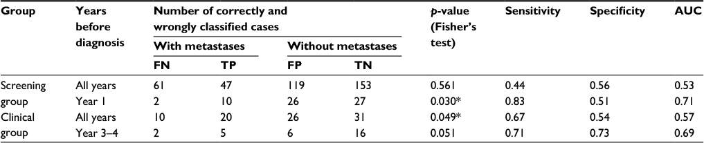Table 4 Number of correctly and wrongly classified cases in the screening group and the clinical group Note: *p-value<0.05. Abbreviation: AUC, area under the curve.

To examine whether the probability of correctly classifying the status of the cases varies with time, we plotted the prediction results against time in Figure 5. For the screening group, we observe that the probability of correct classification is much higher in year 1 before diagnosis. For this period, the p-value obtained using Fisher’s test is equal to 0.030 (Table 4). This is in accordance with the results shown in Figure 3 for the statistic w_p,(g), where we observe that the cases with and without metastases are differentially expressed for some genes in some periods that are close to the time of diagnosis (H0-node). For the clinical group, we observe that the probability of correct classification is much higher in year 3 before diagnosis. For year 3 and 4, the p-value obtained using Fisher’s test is equal to 0.051 (Table 4), while for year 3 it is 0.00 (year 3 contains only 10 case-control pairs where two are with metastases – all 10 cases were correctly classified). Also for the clinical group, the results are in accordance with Figure 3 as the cases with and without metastases are differentially expressed close to year 3 before time of diagnosis (H0-node).

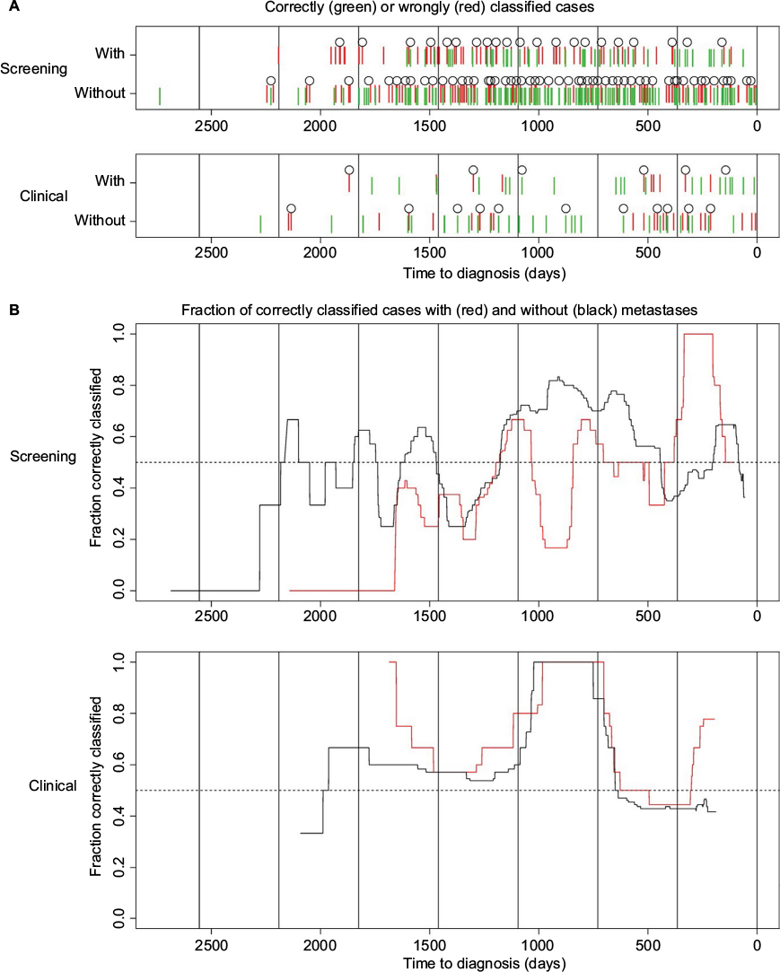Figure 5 Prediction results. Notes: (A) Correctly (green) or wrongly (red) classified cases plotted against time to diagnosis for the screening (upper panel) and the clinical group (lower panel). A circle is plotted above every fifth case. Long vertical lines are plotted to indicate the years. Cases with metastases are plotted on the line labeled “With”, while cases without metastases are plotted on the line labeled “Without”. (B) Fraction of correctly classified cases with (red) and without (black) metastases over time for the screening (upper panel) and the clinical group (lower panel). The fraction for each point in time is computed using a moving window of 1 year (clinical) or 100 days (screening). The resulting curve is then smoothed using a median filter with a window size of 1 year (clinical) or 100 days (screening).

Table 5 shows the top 10 differentially expressed genes, in both the screening and the clinical groups, when comparing cases with and without metastases. In these analyses, the cases were selected from the time period centered around 0.5 years (screening group) and around 2.5 years (clinical group) before diagnosis. We observe that all genes were upregulated in cases with metastases.

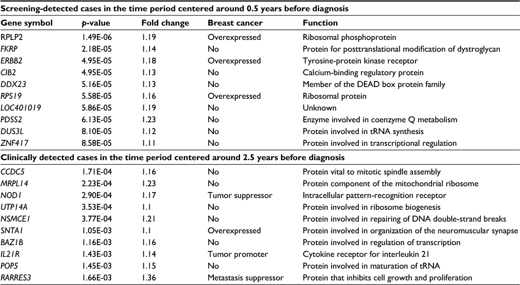Table 5 Top 10 differentially expressed genes in clinically and screening-detected cases when comparing cases with metastases to cases without metastases Note: Genes were sorted by p-value.

We also performed a receiver operating characteristic (ROC) curve analysis (Table 4; Figure 6) by varying the threshold c used when predicting the metastasis status of the cases. In the rightmost column of Table 4, we observe that the area under the curve (AUC) is too close to 0.5 when all years are included. However, for the best period for each group (year 1 for screening, year 3–4 for clinical), fair AUC values around 0.7 were obtained. Figure 6 shows the corresponding ROC curves.

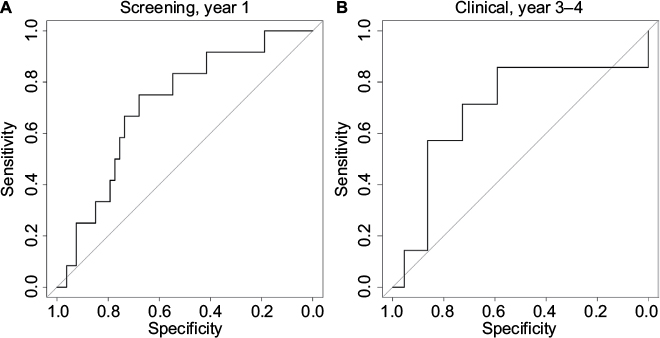Figure 6 ROC curves. Notes: ROC curves obtained when predicting the metastasis status of the cases. (A) ROC curve for the screening group in year 1 before diagnosis. (B) ROC curve for the clinical group in year 3–4 before diagnosis. Abbreviation: ROC, receiver operating characteristic.

We have examined how the score is influenced by n, ie, the number of genes included in the score, for the period with best prediction results using a leave-one-out approach. We observed (Figure S1) that there is a distinct difference in the score between cases with and without metastases, and that the score stabilizes when the number of genes increases. Note that correct predictions are obtained when the scores for the cases with metastases are positive, and the scores for the cases without metastases are negative. It is difficult to conclude how many genes to include in the score to optimize the power of the predictor, but at least 20–50 genes seem to be needed. To find out more about how sensitive the predictor is to the choice of n, we repeated the analyses in Table 4 and Figure 5 with n=50.²⁴ We observed that we obtain results that are similar to the results obtained with n=1000, indicating that the predictor is not very sensitive to the number of genes included in the score when n is at least 50.

Note that the dataset includes seven case-control pairs where the control later was diagnosed with breast cancer. Very similar results were obtained when excluding these seven pairs from the analyses (data not shown).

Discussion

For the first time, using a new statistical method, LITS, we have shown that gene expression profiles in blood demonstrate time-dependent changes related to the phenotype (metastases or not) of the cancer disease and the method of diagnosis (screening versus clinical). Further, the prediction of metastases indicates important time-related changes in the immune system that reflect the final steps of carcinogenesis. These findings could be important building blocks for a human model of carcinogenesis.²⁸ Furthermore, if confirmed in future studies, these signals could serve as biomarkers for advanced stages of cancer, even at the time of diagnosis of the primary tumor. Blood samples that allow measurements of disease biomarkers are also known as liquid biopsies, a term that highlights their use as relatively cheap and non-invasive alternatives to other diagnostic methods such as tissue biopsies and CT or MRI scanning.

The use of moving windows has made this statistical approach more flexible than the curve group analyses that was based on hypotheses of defined time-dependent changes in gene expression or defined curve trajectories.¹⁶ Since this method is not based on the agnostic approach²⁹ that has been used for analyses of single genes or single nucleotide polymorphisms in genome-wide association studies, it evades the conservative procedure of computing p-values with the use of FDRs.^20,30 The approach can be viewed as an effective method for dimension reduction in studies of functional genomics. The analyses of the gene expression profiles are not dependent on the individual testing of the curves for the more than 8000 expressed genes; thus, it mostly eliminates the FDR of multiple testing. The prediction of metastases also indicates that the use of proportional hazard models or linear models will not fit the data and could override the time-dependent changes in gene expression.

When we stratified the data based on the detection category and lymph node status, we found a significant prediction of metastases 3–4 years before diagnosis of a clinical cancer, but only 1 year for a screening-detected cancer. This is compatible with earlier estimations of sojourn time in the screening program. It has been estimated that the introduction of population-based breast cancer screening in Norway gave a mean sojourn time for invasive cancer of 4.0 years in women aged 50–59 years and 6.6 years for those 60–69 years.³¹ Analyses of breast carcinogenesis as a time-dependent process should therefore take into consideration that cases diagnosed within the screening program are diagnosed at an earlier phase of carcinogenesis and thus are not directly comparable to clinically detected cases.

The prospective analyses of gene expression levels in the years preceding breast cancer diagnosis as assessed by the log-fold change between cases and controls showed significant differences after stratification by lymph node status and detection category. Interestingly, all the top 10 differentially expressed genes associated with either clinically or screening-detected metastatic breast cancer were upregulated. This could indicate a higher state of alertness in the cells of the immune system circulating in the blood stream during the years before diagnosis, when comparing those cases with metastases to those without. Furthermore, the analyses showed the ability to discriminate between different stages of the carcinogenic process. A previous analysis of a case-control study within NOWAC showed that differences in blood gene expression profiles reflect both immune responses and aspects of the carcinogenesis.³² The analyses of trajectories could help to understand the time-dependent interaction between the immune response and carcinogenesis. Our findings should be further interpreted in relation to the biology of both single genes and pathways.

Studies of gene expression levels in peripheral blood are challenging and have many difficulties and pitfalls. The transcriptomes of samples in a majority of biobanks are subject to degradation by RNase, which reduces the quality of mRNA for whole-genome analyses. Hence, buffering with RNA stabilizers or snap freezing in liquid nitrogen is necessary to perform transcriptomics in blood samples. The signals related to carcinogenesis in the blood are expected to be much weaker than those in tumor tissues, and can be disturbed by signals from exposures to carcinogens or other lifestyle factors. Furthermore, our approach is challenged by the complexity of studying carcinogenesis in humans, the need for an adequate epidemiological design including exposure information and blood sampling, technical noise in the data, and the development of robust statistics. The prospective design of our study made it difficult to increase the statistical power; so, our results should be interpreted with care.

To the best of our knowledge, the NOWAC Post-genome Cohort is one of the largest population-based prospective cancer studies designed for transcriptomics, owing to the availability of blood samples with preserved gene expression profiles. In the NOWAC Post-genome Cohort, a single laboratory processed all samples using the same technology, thus reducing analytical bias and batch effects. The cohort design reduced selection bias. A weakness of a prospective study could be possible changes in case-control status as controls may become cases as time passes, thus reducing the differences in gene expression levels within a case-control pair. A non-prospective study would suffer from the same issues and in addition there would be no option for time-dependent analyses. We considered as ineligible all case-control pairs in which controls were diagnosed with breast cancer or any other cancer within 2 years of blood sampling. Lastly, there was no repeated sampling of blood, and no additional questionnaires were completed. Repeated measurements would improve the analyses, making it possible to use intra-individual comparisons.

Conclusion

The proposed statistical method, LITS, is sensitive for describing and testing non-linear associations. Our findings could be viewed as a proof of concept of systems epidemiology, indicating the potential to include transcriptomics for functional analysis in prospective studies of cancer.¹⁵ Overall, these results contribute to building a more complete model of the carcinogenic process in humans.

Acknowledgments

We are thankful to and impressed by the women who donated blood for this cancer research project. Bente Augdal, Merete Albertsen, and Knut Hansen were responsible for all infrastructure and administrative issues. We thank Clara-Cecilie Günther for preprocessing the data. This study was supported by a grant from the European Research Council (ERC-AdG 232997 TICE). The funders had no role in the design of the study; in the collection, analyses, and interpretation of the data; in the writing of the manuscript; or in the decision to submit for publication. Some of the data in this article are from the Cancer Registry of Norway. The Cancer Registry of Norway is not responsible for the analysis or interpretation of the data presented. Microarray service was provided by the Genomics Core Facility, Norwegian University of Science and technology, and NMC – a national technology platform supported by the functional genomics program (FUGE) of the Research Council of Norway. The data will be stored at the European Genome-phenome Archive (EGA, https://www.ebi.ac.uk/ega/),³³ where it will be accessible on request.

Author contributions

All authors contributed toward data analysis, drafting and revising the paper and agree to be accountable for all aspects of the work.

Disclosure

The authors report no conflicts of interest in this work.

References

1.		International Agency for Research on Cancer. GLOBOCAN 2012: Estimated cancer incidence, mortality and prevalence worldwide in 2012. Available from: http://globocan.iarc.fr/. Accessed June 22, 2017.
2.		Todd M, Shoag M, Cadman E. Survival of women with metastatic breast cancer at Yale from 1920 to 1980. J Clinl Oncol. 1983;1(6):406–408.
3.		Cancer in Norway 2012. Cancer incidence, mortality, survival and prevalence in Norway. Oslo: Cancer Registry of Norway, 2014. Available from: https://www.kreftregisteret.no/globalassets/cancer-in-norway/2012/cin_2012-web.pdf. Accessed June 22, 2017.
4.		Lipscomb J, Fleming ST, Trentham-Dietz A, et al; Centers for Disease Control and Prevention National Program of Cancer Registries Patterns of Care Study Group. What predicts an advanced-stage diagnosis of breast cancer? Sorting out the influence of method of detection, access to care, and biologic factors. Cancer Epidemiol Biomarkers Prev. 2016;25(4):613–623.
5.		Turajlic S, Swanton C. Metastasis as an evolutionary process. Science. 2016;352(6282):169–175.
6.		Vineis P, Schatzkin A, Potter JD. Models of carcinogenesis: an overview. Carcinogenesis. 2010;31(10):1703–1709.
7.		Rangarajan A, Weinberg RA. Opinion: comparative biology of mouse versus human cells: modelling human cancer in mice. Nat Rev Cancer. 2003;3(12):952–959.
8.		Of men, not mice. Nat Med. 2013;19(4):379.
9.		Gould SE, Junttila MR, de Sauvage FJ. Translational value of mouse models in oncology drug development. Nat Med. 2015;21(5):431–439.
10.		Freedman ML, Monteiro AN, Gayther SA, et al. Principles for the post-GWAS functional characterization of cancer risk loci. Nat Genet. 2011;43(6):513–518.
11.		Chadeau-Hyam M, Athersuch TJ, Keun HC, et al. Meeting-in-the-middle using metabolic profiling - a strategy for the identification of intermediate biomarkers in cohort studies. Biomarkers. 2011;16(1):83–88.
12.		Cava C, Bertoli G, Castiglioni I. Integrating genetics and epigenetics in breast cancer: biological insights, experimental, computational methods and therapeutic potential. BMC Syst Biol. 2015;9:62.
13.		Arnedos M, Vicier C, Loi S, et al. Precision medicine for metastatic breast cancer – limitations and solutions. Nat Rev Clin Oncol. 2015;12(12):693–704.
14.		Cesar ASM, Gradishar WJ. Changing treatment paradigms in metastatic breast cancer: lessons learned. JAMA Oncol. 2015;1(4):528–534; quiz 549.
15.		Lund E, Dumeaux V. Systems Epidemiology in Cancer. Cancer Epidemiol Biomarkers Prev. 2008;17(11):2954–2957.
16.		Lund E, Holden L, Bøvelstad H, et al. A new statistical method for curve group analysis of longitudinal gene expression data illustrated for breast cancer in the NOWAC postgenome cohort as a proof of principle. BMC Med Res Methodol. 2016;16:28.
17.		Lund E, Plancade S, Nuel G, Bøvelstad H, Thalabard JC. A processual model for functional analyses of carcinogenesis in the prospective cohort design. Med Hypotheses. 2015;85(4):494–497.
18.		Holden L. Time development of gene expression. NR note SAMBA/35/15, 2015. Available from: https://www.nr.no/files/samba/smbi/note2015SAMBA3515timeDevelopmentGenes.pdf. Accessed June 22, 2017.
19.		Holden L. Classify strata. NR note SAMBA/11/15, 2015. Available from: https://www.nr.no/files/samba/smbi/note2015SAMBA1115classifyStrata.pdf. Accessed June 22, 2017.
20.		Reiner A, Yekutieli D, Benjamini Y. Identifying differentially expressed genes using false discovery rate controlling procedures. Bioinformatics. 2003;19(3):368–375.
21.		Lund E, Dumeaux V, Braaten T, et al. Cohort profile: The Norwegian Women and Cancer Study–NOWAC–Kvinner og kreft. Int J Epidemiol. 2008;37(1):36–41.
22.		Dumeaux V, Borresen-Dale AL, Frantzen JO, Kumle M, Kristensen VN, Lund E. Gene expression analyses in breast cancer epidemiology: the Norwegian Women and Cancer postgenome cohort study. Breast Cancer Res. 2008;10(1):R13.
23.		Hofvind S, Geller B, Vacek PM, Thoresen S, Skaane P. Using the European guidelines to evaluate the Norwegian Breast Cancer Screening Program. Eur J Epidemiol. 2007;22(7):447–455.
24.		Holden M, Holden L. Statistical analysis of gene expression in blood before diagnosis of breast cancer. NR note SAMBA/07/16, 2016. Available from: https://www.nr.no/files/samba/smbi/note2016SAMBA0716BreastCancer.pdf. Accessed June 22, 2017.
25.		Lin SM, Du P, Huber W, Kibbe WA. Model-based variance-stabilizing transformation for Illumina microarray data. Nucleic Acids Res. 2008;36(2):e11.
26.		Du P, Kibbe WA, Lin SM. nuID: a universal naming scheme of oligonucleotides for Illumina, Affymetrix, and other microarrays. Biol Direct. 2007;2:16.
27.		Du P, Feng G, Kibbe W, Lin S (2016). lumiHumanIDMapping: Illumina Identifier mapping for Human. R package version 1.10.1.
28.		Lund E, Plancade S. Transcriptional output in a prospective design conditionally on follow-up and exposure: the multistage model of cancer. Int J Mol Epidemiol Genet. 2012;3(2):107–114.
29.		Spitz MR, Bondy ML. The evolving discipline of molecular epidemiology of cancer. Carcinogenesis. 2010;31(1):127–134.
30.		Berry D. Multiplicities in cancer research: ubiquitous and necessary evils. J Natl Cancer Inst. 2012;104(15):1124–1132.
31.		Weedon-Fekjær H, Lindqvist BH, Vatten LJ, Aalen OO, Tretli S. Estimating mean sojourn time and screening sensitivity using questionnaire data on time since previous screening. J Med Screen. 2008;15(2):83–90.
32.		Dumeaux V, Ursini-Siegel J, Flatberg A, et al. Peripheral blood cells inform on the presence of breast cancer: a population-based case-control study. Int J Cancer. 2015;136(3):656–667.
33.		Lappalainen I, Almeida-King J, Kumanduri V, et al. The European Genome-phenome Archive of human data consented for biomedical research. Nat Genet. 2015;47(7):692–695.

Supplementary material

Method

Adjusting for the batch effect

Here, we give a short description of the ComBat method developed by Johnson et al¹ for estimating the batch effects and how to use these estimates for adjusting for the batch effects when computing sample means and standard deviations.

The log₂ gene expression value Y_ijg for gene g and sample j from batch i is modeled as

where

• α_g is the overall gene expression,
• X is a design matrix for sample conditions,
• β_g is the vector of regression coefficients corresponding to X,
• γ_ig is the additive batch effect, and
• δ_ig is the multiplicative batch effect.

The batch-adjusted data Y_ijg can then be computed as

.

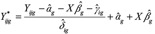The estimates of the parameters α_g, β_g, γ_ig, and δ_ig are computed using an empirical Bayes method.¹ Note that in the implementation of the method, the batch-adjusted data Y_ijg are computed as 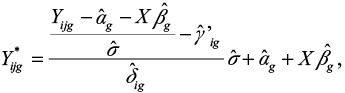where is the parameter that is estimated instead of .

Both the expectation and the variance of a gene for the cases can vary both with time and stratum. We therefore cannot use the ComBat method for batch adjusting the dataset that consists of differences in log₂ gene expression between cases and controls. Instead we will use ComBat to estimate the batch effects and from a dataset that includes only the log₂ gene expressions for the controls.

Log₂ gene expression data that are adjusted for the additive batch effect γ_ig, but not for the multiplicative batch effect δ_ig, can then be computed as

For case-control pair c from batch i with sample j₁ as control (from group G1) and sample j₂ as case (from group G2), we have the log₂-expression difference of X_g,c.

We observe that X_g,c is adjusted for the additive batch effect γ_ig, but not for the multiplicative batch effect δ_ig.

We compute the estimate of μ_g, as the weighted average of X_g,c, where the weights are , and we compute the estimate of 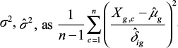. We will compare estimated sample means and standard deviations between genes. For each gene, we therefore multiply the estimates of by a constant so that for this gene , where B is the number of batches/runs.

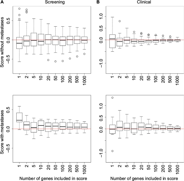Figure S1 Boxplots illustrating how the score used in the predictor depends on the number of genes included in the score. Notes: The score has been normalized by dividing with the number of genes included in the score. The score for the cases with metastases should be positive (lower panel), while the scores for the cases without metastases should be negative (upper panel). (A) Scores for case-control pairs around 6 months from the screening group. (B) Scores for case-control pairs around 2 years and 6 months from the clinical group.

Reference

1.

Johnson WE, Li C, Rabinovic A. Adjusting batch effects in microarray expression data using empirical Bayes methods. Biostatistics. 2007;8(1):118–127.