Does ethylene gas collapse on polymerization to polyethylene?

Introduction

The mathematics that governs the equilibrium statistical mechanics of polymer molecules in dilute solution is well studied for the past many decades.¹ If we consider a single polymer chain in isolation, we have to deal with two scenarios: the polymer chain in (a) good solvent and (b) poor solvent. In good solvent, the only interaction between the atoms of the polymer chain is repulsion, and this is best modeled by the self-avoiding walk. This explains in a satisfactory way the critical exponent of mean square end-to-end distance (radius of gyration) obtained from experiment. In poor solvent, there are two types of interactions between atoms in the polymer chain, repulsion and attraction. This is best modeled by the use empirical potentials such as Lennard–Jones potential (LJP) and Kihara-type potentials. The salient feature of the use of this potential in the calculation of the mean square end-to-end distance is the existence of a phenomenon called polymer collapse that is also observed experimentally.^2,3 The collapse of the chain from a coil to globular structure is observed for the chain as a whole and also locally at certain portions of the chain.^2,3

Polymerization commonly occurs by means of two reaction mechanisms: (a) addition and (b) condensation. Calculations of the mean square end-to-end distance on growing polymer chains undergoing addition polymerization in good solvent (repulsion interaction only) were extensively carried out ~30 years ago.^4–6 However, no calculations have been carried out on growing polymer chains using potentials for both attraction and repulsion. Recently, the model for addition polymerization was extended to accommodate condensation polymerization⁷ using the depth first-search technique.⁸ In this paper, we describe calculations on the growth of polyethylene (PE) from ethylene gas by chain or addition polymerization. Similar calculations on polymer chains growing by the condensation mechanism under the influence of both attraction and repulsion have also been carried out.⁹

Our calculations on PE reveal that the phenomenon of polymer collapse will occur only after the reaction is complete. This is explained in terms of the fact that the probability distribution for equilibrium statistical mechanics of the polymer chain (uniform probability distribution) is different from the probability distribution of polymer chains that grow by addition polymerization (growing self-avoiding walk distribution [GSAW]), the time scales for reorientation at equilibrium and nonequilibrium being vastly different. To reinforce this argument, we examine a statistic that has recently been studied in detail, the atmosphere of self-avoiding walks and polymer chains.

The atmosphere in self-avoiding walks and GSAWs

The existence of the connective constant for self-avoiding walks , where c_n is the cardinality of the set of self-avoiding walks of n steps, has been known for many decades now.¹ However, the past decade has seen the development of highly sophisticated Monte Carlo (MC) algorithms to estimate this quantity to a high degree of accuracy.^10–12 These authors have defined the atmosphere of a self-avoiding walk as the number of vacant (unoccupied) sites available for growth of an n-step self-avoiding walk. It is seen that the expectation of the atmosphere in self-avoiding walks is given by , where c_n is the cardinality of the set of self-avoiding walks of n steps. All algorithms mentioned earlier are improvements of the Rosenbluth and Rosenbluth algorithm first proposed ~50 years ago.¹³ The Rosenbluth and Rosenbluth algorithm samples from a probability distribution that is based on the atmosphere of the walk and is hence different from the uniform distribution and then uses an estimated weight factor to extrapolate statistics obtained from these calculations to those expected from the uniform distributions. Improvements such as the (i) pruned and enriched Rosenbluth sampling, (ii) flat histogram Rosenbluth sampling, and the (iii) generalized atmospheric Rosenbluth sampling all use a similar weighting technique to extrapolate to the uniform distribution.^10–12

Statistics estimated by the probability distribution that is based on the atmosphere of a self-avoiding walk is important for the following reason.

It is well established that the kinetics of polymerization (growth of a polymer molecule) depends on the fast motions of what is usually called the head of the molecule.¹⁴ It is also well established experimentally that the fast and slow motions of the polymer molecule in dilute solution in a good solvent differ by a very large order of magnitude.^15,16 What this implies (if we assume Gibb’s hypothesis that the time average is equal to the ensemble average is true) is that while the equilibrium statistics of a polymer in dilute solution in a good solvent obey the uniform distribution, the statistics of a growing polymer chain in dilute solution obey a distribution that is based on the atmosphere of the growing molecule. Since the polymerization is an extremely fast reaction, there is little scope at present for experimental verification that the average dimensions of a growing polymer molecule in the gas phase or in solution remain the same after the reaction is complete. Hence, it is necessary to study the statistics of a GSAW (kinetically growing walks).

A unified model for self-avoiding walks growing by addition and condensation polymerization was recently proposed.⁷ In this model for an n-step self-avoiding walk P_n, we define λ(P_n) as the average number of vacant lattice sites available to the walker as he starts from the origin until he reaches the site occupied by the terminal step and μ_U(n) as the expectation of this average, where probabilities are calculated according to the uniform distribution, and μ_G(n) as the expectation of this average where probabilities are calculated according to the GSAW distribution. In this paper, we report values of μ_G(n) and μ_U(n) by exact enumeration for two and three dimensions and observe that the expectation and standard deviation of the average atmosphere are different for both types of walks. This difference in the probability distribution is used to explain the absence of polymer collapse in kinetically growing PE.

Methods

Definitions and theory

In an earlier paper,⁷ we had defined the probabilities for self-avoiding walks that grow by looking ahead by an arbitrary number of steps ahead. We define the same quantities of walks looking only one step ahead as follows.

Let S_i+1 be the set of self-avoiding walks of i+1 steps starting at the origin. Let P_i = p(0), …, p(i) be the sites of an i-step self-avoiding walk starting at the origin. Let F_i+1(P_i) denote the subset of walks in S_i+1 for which P_i = p(0), …, p(i) are the first i+1 sites and |F_i+1(P_i)| is the cardinality of this subset. Let P_i+1′ = p(0), …, p(i), p(i + 1) be the sites of an i+1-step self-avoiding walk starting at the origin whose first i+1 sites are (0), …, p(i).

We now define the probability of the i+1 step being along sites p_i and p_i+1 in a GSAW as:

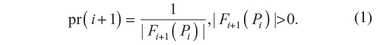
where pr(i+1) is a conditional probability. It is the probability of the i+1th step being along sites p_i and p_i+1, given that the walk has survived up to i steps. The probability of the walk P_n+1′ = p(0), …, p(n), p(n + 1) defined in terms of the GSAW model is given by:

where pr(i) is given by Equation 1.

We now define a random variable 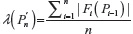, where |F_i(p_i–1)| is defined in Equation 1 with |F₁(P₀)| = 2d, where P₀ is the origin and d is the dimension of the lattice. The expectation of λ under the GSAW is given by: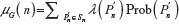, where is given in Equation 2. Similarly, expectation of λ under the uniform distribution is given by: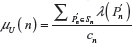, where c_n is the cardinality of the set of n-step self-avoiding walks. To illustrate further, we calculate μ_G(4) and μ_U(4) in two dimensions as follows:

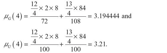
We further define: μ_G = lim_n→∞λG (n) and μ_U = lim_n→∞λU (n). In this paper, compare μ_G and μ_U with the connective constant .

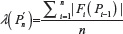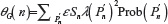For the purpose of the afore mentioned comparison, we also need the standard deviations related to μ_U(n) and μ_G(n) We therefore, define the second moment of as and 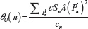, giving for the standard deviation: 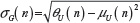and .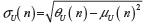

The model used for PE

We have chosen to use the united atom/Ryckaert–Bellmans¹⁷ model for isolated PE chains. In this model, each atom “i” in the chain is characterized by a Lennard–Jones 12-6 potential given by

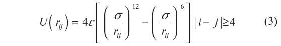
Here, r_ij is the distance between the ith and jth atoms, ε/k_B =72 K and σ=3.923 Å. While the LJP accounts for the non-bonding interactions in the chain, the local interactions are taken care of by the torsional potential given by:

where k_B is the Boltzmann’s constant, Φ_i is the ith torsion angle, and a₀=1.157, a₁=1.515, a₂=–1.636, a₃=–0.382, a₄=3.271, and a₅=–3.927.

The LJP is used to model the bare skeletal carbon backbone in PE. We have also used another potential function, known as the Kihara convex core potential (KCCP),¹⁸ to model the PE chain with the hydrogen atoms included in the backbone. Like the LJP, the Kihara potential takes the form

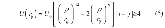
where U₀/k_B =223 K and ρ = 3.15 Å. Irrespective of the potentials for non-bonding interactions, the bonding (local) interactions between nearest neighbor monomers are calculated using Equation 4. The bond length is taken as l=1.53 Å. For simulation using LJP, the bond angle complement θ=70.53°, while for the simulation using Kihara potential, θ=68° (as proposed by Flory¹⁴). This difference in the use of θ is due to the fact that we carried out the simulation using LJP to compare with the work of earlier authors¹⁹ and hence used the parameters taken by them. In the light of Flory’s rotational isomeric state approximation, Φ =0°, +120°, and –120°. For the purposes of comparison, we use the united atom model followed by earlier authors,¹⁹ where five rather than three terms are used. As explained in the next section, the same cutoff for rejection has also been used by us.

An average of 60 independent samples were used for the MC simulation for calculations involving both the KCCP and LJP for both probability distributions with sample sizes taken large enough so that the standard deviation/mean in all cases was <0.01%. This ensured that we had a good convergence at higher number of bonds.

The present work involves modeling of real polymer chains that are growing or, in other words, reacting. We use the uniform probability distribution and a probability distribution, known as GSAW, in our simulation. Again, we have used two potential functions, LJP and KCCP, to model the non-bonding interactions between the chain segments. Thus, we get two sets of results, one using the LJP and the other using KCCP with each of these probability distributions. In addition, the calculations using KCCP have been carried out at four temperatures, ie, 1,000, 413, 298, and 100 K. Both exact enumeration and MC simulation have been carried out for each of these.

At the beginning of the calculation, the configuration is set to the all-trans chain. The all-trans configuration is the one with the lowest local energy, while the configuration with alternate gauche conformations has the highest. In our program, the digit “0” represents a trans conformation (Φ=0°), “1” for gauche+ conformation (+120°), and “2” for gauche– (–120°) conformation. Hence, an all-trans chain of N bonds may be represented by a series of N–2 zeroes (starting with the second bond up to N–1th bond). Certain parameters such as the temperature T, θ, ρ or σ, U₀ or ε, and the gas constant R are all defined outside the main program. An outline of the steps involved in both programs is discussed in brief.

Uniform probability distribution

Exact enumeration

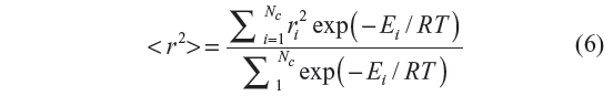
For a given number of bonds N, the exact enumeration method involves the generation of 3^N–2 configurations starting with the initial all-trans configuration. For each such configuration, its total energy is calculated as the sum of local and non-local energies. The statistical weight thus determined is multiplied to the square of the end-to-end distance of the configuration. Once all of the 3^N–2 configurations are generated, the mean square end-to-end distance and the characteristic ratio are calculated using Equations 6 and 7, respectively, with N_c=3^N–2.

The characteristic ratio c_n is given by:

MC simulation

In the MC simulation using uniform distribution, each sample is generated starting from the beginning by random step-by-step sampling of the torsion angles. Each of the torsion angles (0, +120, or –120) is selected with equal probability, and a complete N-mer chain is constructed in sequence. Once a chain is built up, its atomic coordinates are generated for N+1 atoms. The local energy which takes care of interactions up to four skeletal bonds is calculated using Equation 2, for the whole chain. The distance between atoms “i” and “j” is calculated for every pair i, j such that |i–j|≥4. Configurations in which any pair of atoms are at a distance less than l+σ (1.53+3.923 Å for LJ and 1.53+3.15 Å for Kihara) are rejected.¹⁹ These values are passed on to another subroutine where the non-local energies, operative between all chain segments that are further apart by four or more skeletal atoms, are calculated using either Equation 3 or 4 depending on the potential function used. Sum of the local and non-local energies of a particular chain gives its total energy E, that is, E = E_L + E_NL. Using E, the statistical weight of the configuration is calculated as exp(− E / k_BT) or exp (− E / RT) (depending on the units used for E), where R is the universal gas constant.

The end-to-end distance “r” of the generated configuration is calculated which is squared and then multiplied with the statistical weight corresponding to that configuration. If N_c is the total number of chains generated (sample size) during the simulation, then the ensemble average of the mean square end-to-end distance is given by Equation 6, and the characteristic ratio C_n by Equation 7.

GSAW probability distribution

Exact enumeration

Starting with the all-trans configuration, all of the 3^N–2 configurations are generated. During the generation of each configuration, at each bond position, the following steps are performed. Each bond position is attempted with the 0, 1, and 2 conformations. The second bond position is set at 0 (by symmetry considerations). The third bond position is tried with 0, 1, and 2. For every attempt at a bond position, the statistical weight is calculated. The sum of the three statistical weights at each bond position is also computed. The statistical weight corresponding to the conformation being sampled divided by the sum of the three statistical weights gives the probability of selection of that conformation at that bond position. This probability is stored. The process is repeated for N–2 bonds in a configuration, each time generating the probability. Finally, we get a product of these N–2 probabilities which is the total probability of that configuration, say Tot_P. The sum of the squares of the end-to-end distance, r², for each configuration is multiplied with its Tot_P. This whole procedure is repeated for 3^N–2 configurations. The mean square end-to-end distance is then computed as

MC simulation

Here again, each sample is generated by starting with the torsional angle of the third bond. In GSAW, we sample ahead by one bond position. The third bond position is selected by calculating the E_t for the three rotational isomeric states using Equation 2. Their corresponding weights are determined using the equation exp(− E_t / RT). A random number is generated which is compared with the probabilities (statistical weight of each state divided by the sum of the statistical weights) for the three states, and the third bond position is selected accordingly in a random fashion. Its coordinates are then generated. From the fourth bond onward up to N–1th bond, each bond position is attempted with each of the three states, and during each attempt, atom coordinates are generated along with the total energy and the corresponding statistical weight. The statistical weight corresponding to a particular state divided by the sum of the three statistical weights gives the probability of that conformation at the bond position. A random number is generated which is compared with each of these probabilities, and the bond conformation at that position is selected. This process is repeated until N–2 bond conformations are generated by this procedure. Configurations in which any pair of atoms are at a distance less than l+σ (1.53+3.923 Å for LJ and 1.53+3.15 Å for Kihara) are rejected.¹⁹ The end-to-end distance square is calculated for that particular configuration. In this manner, N_c chains are generated, and their end-to-end distance squared, r², values are summed up. The mean square end-to-end distance is calculated as

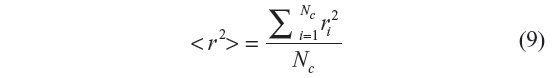
and the characteristic ratio c_n is calculated as given in Equation 7.

To sum up briefly: In the GSAW probability distribution, each of the N–2 bond positions is attempted with 0, 1, and 2 conformations. During each such attempt, we sample one bond position ahead. Suppose the second bond is set with the conformation 0. For the third bond position, the statistical weight determined from the local energy calculations as per Equation 2 is stored in, say, w [0], w [1], and w [2]. Now, w [0]/(w [0] + w [1] + w [2]) gives the probability of the conformation 0 at that bond position. Similarly, the other two probabilities are computed. A random number is then generated which is compared with each of these probabilities and a conformation is selected randomly for that bond position. This process is repeated for the N–1 remaining bonds when a configuration sample is said to be generated. The square of the end-to-end distance of that configuration is calculated. Using this technique, N_c chains are generated, and their end-to-end distance squared value, r², is summed up.

Results and Discussion

We use the depth first-search algorithm described in earlier papers^7,8 to calculate values of μ_G(n), σ_G(n), μ_U(n), σ_U(n), and in two and three dimensions. For such an algorithm that uses the depth first-search tree, the number of vertexes at each level of the tree is equal to the number of self-avoiding walks for the number of steps equal to that level. Here, the level of a vertex in a tree is the length of the path from the root of the tree to that vertex. If we use the notation used in Ref. 1 (borrowed from genealogy), 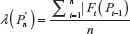represents the average number of children of each vertex along the path from the root of the tree to the vertex at the n–1th level (including the 2d children of the root). That is, the average number of children along the path from the root to the vertex in question, excluding the number of children of that vertex (leaf). The advantage in using this algorithm is that we need only single run of the program that uses this algorithm to calculate μ_G(n), σ_G(n), μ_U(n), σ_U(n), and simultaneously.

Results of exact enumeration for two and three dimensions

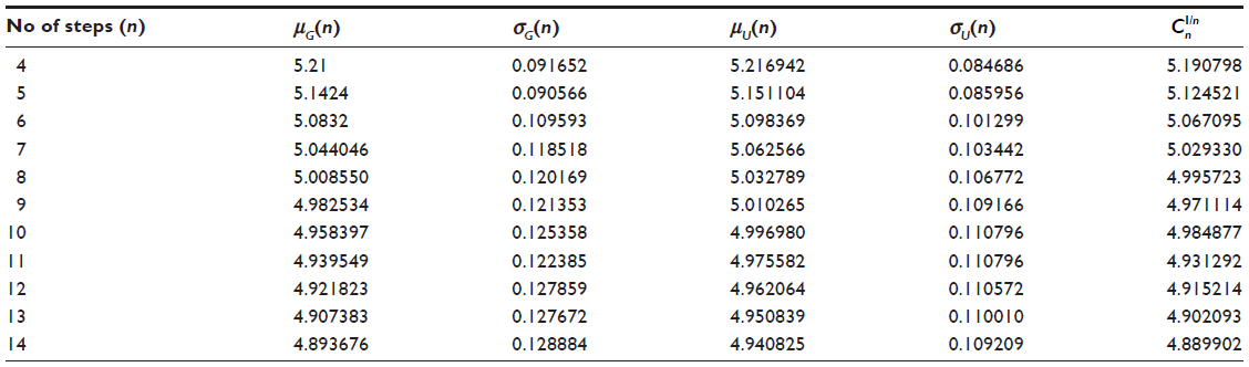
In Table 1, we report exact enumeration values of μ_G(n), σ_G(n), μ_U(n), σ_U(n), and in two dimensions. In Table 2, we report exact enumeration values of μ_G(n), σ_G(n), μ_U(n), σ_U(n), and in three dimensions.

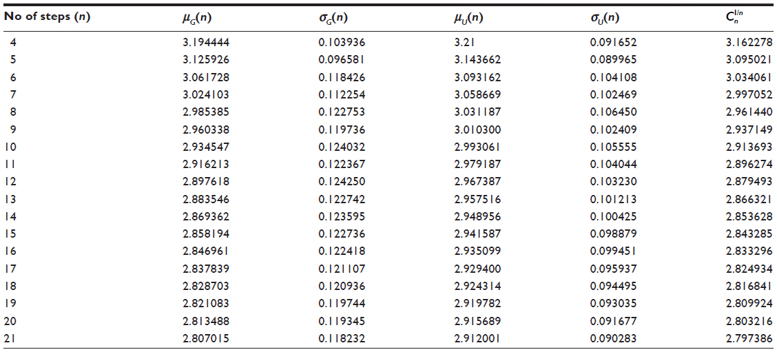Table 1 Exact values of μG(n), σG(n), μU(n), σU(n), and in two dimensions

Table 2 Exact values of μG(n), σG(n), μU(n), σU(n), and in three dimensions

Results of real PE chain

The results of our computations for the characteristic ratio vs the number of bonds for the uniform probability distribution and GSAW distribution for PE with the LJP at 1,080 K are plotted in Figure 1. This computation was carried out primarily to check our program for the uniform distribution with previously published results.¹² It is clear from Figure 1 that polymer collapse occurs at ~20 bonds for the uniform distribution (in agreement with earlier calculations on the same system), whereas for GSAW, there is no collapse clearly up to 180 bonds.

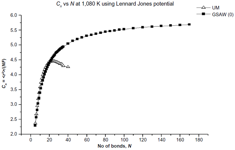Figure 1 Plot of the characteristic ratio vs the number of bonds in PE with LJP at 1,080 K for uniform and GSAW distributions. Abbreviations: PE, polyethylene; LJP, Lennard–Jones potential; GSAW, growing self-avoiding walk; UM, uniform.

In Figures 2–5, we plot the results of our computations for the characteristic ratio vs the number of bonds for the uniform probability distribution and GSAW distribution for PE with the KCCP at 1,000, 413, 298, and 100 K. It is observed that in all cases, polymer collapse occurs between eight and ten bonds (ie, for octane, nonane, or decane) for the uniform distribution, whereas collapse does not occur up to 180 bonds in GSAW in all cases. This implies that we observe polymer collapse for uniform walks in our exact enumeration calculations.

Figure 2 Plot of the characteristic ratio vs the number of bonds in PE with Kihara potential at 1,000 K for uniform and GSAW distributions. Abbreviations: PE, polyethylene; GSAW, growing self-avoiding walk; UM, uniform.

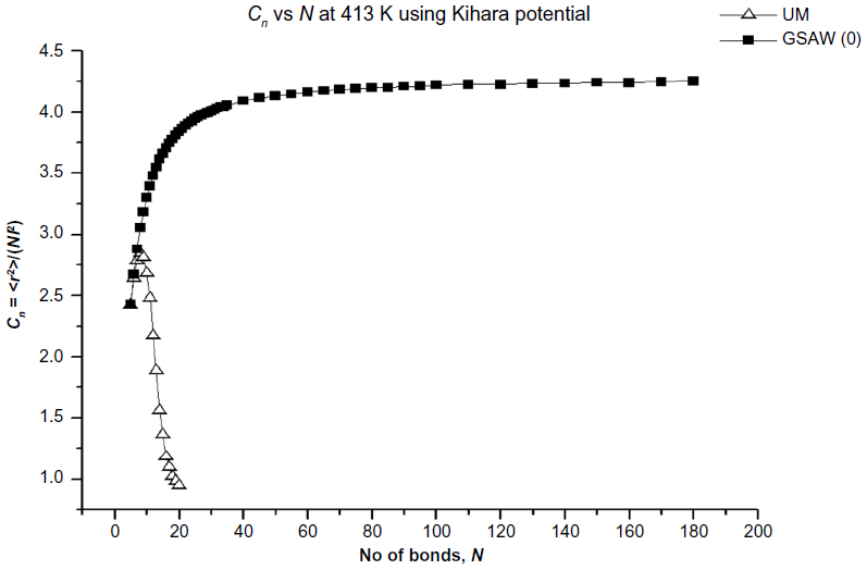Figure 3 Plot of the characteristic ratio vs the number of bonds in PE with Kihara potential at 413 K for uniform and GSAW distributions. Abbreviations: PE, polyethylene; GSAW, growing self-avoiding walk; UM, uniform.

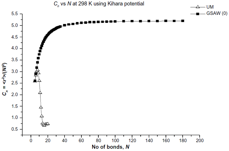Figure 4 Plot of the characteristic ratio vs the number of bonds in PE with Kihara potential at 298 K for uniform and GSAW distributions. Abbreviations: PE, polyethylene; GSAW, growing self-avoiding walk; UM, uniform.

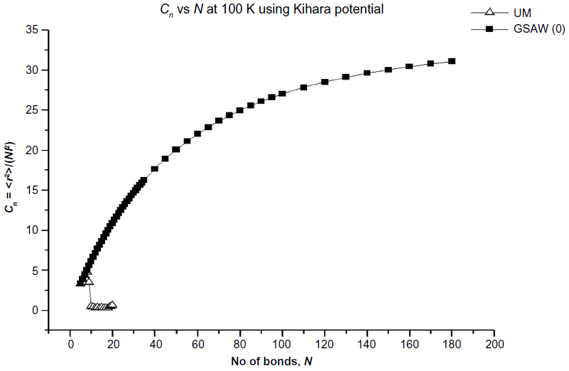Figure 5 Plot of the characteristic ratio vs the number of bonds in PE with Kihara potential at 100 K for uniform and GSAW distributions. Abbreviations: PE, polyethylene; GSAW, growing self-avoiding walk; UM, uniform.

Discussion

It was mentioned at the very beginning of the paper that the mathematics that governs the equilibrium statistical mechanics of polymer molecules in dilute solution is well studied for the past many decades.¹ However, the mathematics of growing polymer chains has not been studied. Moreover, when one studies both experimentally and theoretically the effect of the degree of polymerization (molecular weight), one usually uses samples of increasing molecular weight to study the size. There are no experimental studies that examine the size of polymer molecules as the polymerization proceeds, simply because the reactions are simply too fast to measure the average dimensions such as the mean square end-to-end distance and mean radius of gyration.

The main finding of this study was that the growing PE chains do not collapse, whereas PE chains using KCCP collapse very early (in our exact enumeration computations in all cases). This is a startling finding since what it means is that ethylene gas on polymerizing to linear PE collapses from a coil-like state to a globular state on completion of the reaction. This can be explained by using our exact enumeration calculations in Tables 1 and 2. The probability distributions are totally different. The GSAWs have also been called the “myopic self-avoiding walk”.¹ What this implies is that the growing walker does not see the attractive part of the potential in GSAWs, and hence, polymer collapse is not observed. On the other hand in the uniform self-avoiding walk, the walker sees both the attractive and repulsive part of the potential, and hence, after a certain number of steps, polymer collapse is observed.

As a final point of discussion, the transition that is observed is the converse of that reported by Yamamoto et al^20,21 for crystallization from a globular state to a chain-folded crystallite (eg, Figure 2 in page 1977 in the work of Yamamoto²⁰).

Conclusion

In this paper, we are able to predict that ethylene on polymerizing in the gas phase collapses from a coil-like structure to a globular structure. From a mathematical standpoint, this can be attributed to the fact that the probability distributions governing the statistical mechanics at equilibrium and nonequilibrium are different.

Disclosure

The authors report no conflicts of interest in this work.

---

References

1.	Madras N, Slade G. The Self-avoiding Walk. Boston: Birkhausser; 1993.
2.	Nishio I, Sun ST, Swislow G, Tanaka T. First observation of coil - globule transitions in a single polymer chain. Nature. 1979;281:208–209. doi:10.1038/281208a0.
3.	Nishio I, Sun ST, Swislow G, Tanaka T. Critical density fluctuations within a single polymer chain. Nature. 1982;300:243–244. doi:10.1038/300283a0.
4.	Majid I, Jan N, Conigilio A, Stanley HE. Kinetic growth walk: a new model for linear polymers. Phys Rev Lett. 1985;55(15):1257–1260.
5.	Kremer K, Lyklema JW. Kinetic growth models. Phys Rev Lett. 1984;52(19):2091.
6.	Majid I, Jan N, Congilio A, Stanley HE. Comments and replies to kinetic growth models. Phys Rev Lett. 1985;55(19):2092.
7.	Padmanabhan AS. Growing self avoiding walk trees. J Math Chem. 2014;52(1):355–367. doi:10.1007/S10910-013-0267-z.
8.	Padmanabhan AS, Jacob S. Self avoiding walks and laces. J Math Chem. 2014;52(2):627–645. doi:10.1007/S10910-013-0283-z.
9.	Satheesh N. [Ph.D. thesis]. Kerala: Mahatma Gandhi University; 2013.
10.	Rechnitzer A, Janse van Rensburg EJ. Canonical Monte Carlo determination of the connective constant of self avoiding walks. J Phys A Math Gen. 2002;35:L605–L612.
11.	Owczarek AL, Prellberg T. Scaling of the atmosphere of self avoiding walks. J Phys A Math Theor. 2008:41;37504.
12.	Rechnitzer A, Janse van Rensburg EJ. Generalised atmospheric sampling of self avoiding walks. J Phys A Math Theor. 2008;41:442002.
13.	Rosenbluth MN, Rosenbluth AW. Monte Carlo calculation of the average extension of molecular chains. J Chem Phys. 1955;23:356.
14.	Flory PJ, editor. Principles of polymer chemistry. In: Theory of Reactivity of Large Molecules. New York: Cornell University Press; 1953:75–78.
15.	Hall CK, Helfand E. Conformational state relaxation in polymers: time correlation functions. J Chem Phys. 1982;77(6):3275–3282.
16.	Blum FD, Durairaj B, Padmanabhan AS. Backbone dynamics of poly(isopropyl acrylate) in chloroform. A Deuterium NMR study. Macromolecules. 1984;17:2837–2846.
17.	Ryckaert JP, Bellmans A. Faraday Discuss Chem Soc. 1977;66:95.
18.	Kihara T. Intermolecular Forces. New York: John Wiley; 1978.
19.	Sadanobu J, Goddard WA 3rd. J Chem Phys. 1997;106(16):6722.
20.	Yamamoto T. Computer modeling of polymer crystallization – towards computer assisted materials design. Polymer. 2009;50:1975–1985.
21.	Yamamoto T, Orimi N, Urakami N, Sawada K. Molecular dynamics modeling of polymer crystallization; from simple polymer to helical ones. Faraday Discuss. 2005;128:75–86.