Comparison analysis of separate and joint models in case of time-to-death event of HIV/AIDS patients under ART follow-up

Introduction

In clinical and medical studies, longitudinal and time-to-event data are often considered important measures of health. Most of the time the longitudinal and survival data arise together in practice.^1,2 Longitudinal studies are characterized by observation of repeated measurements on subjects at a series of time points. The time-to-event datum describes the length of time for occurrence of the specified event on each individual. The event time is often dependent on disease marker status, and so joint analysis of survival with repeated measures has been fruitful to capture this dependence.^3,4

Data analyses mostly focus on the longitudinal data or the survival data or both. The longitudinal data analysis focuses on informative dropouts because dropouts are very common in such studies, and the survival data analysis focuses on incorporating time-dependent covariates such as CD4 counts because the time to event may be associated with the covariate trajectories. If the researcher is interested in investigating the association between the two processes, joint models analyses are essential to handle the association between the longitudinal and the survival data.²

Most often joint model analysis uses the proportional hazards (PH) models. However, when the PH assumption is violated, the parametric accelerated failure time (AFT) model is an attractive approach.⁵ Many methods exist for analyzing longitudinal and survival data separately. But separate analyses of such kind of data may lead to inefficient or biased results. This can be improved by joint modeling of the longitudinal and the survival data. Such joint model may provide valid and efficient inferences.⁶

Methods

The population of our study includes all HIV/AIDS patients under antiretroviral therapy (ART) follow-up from January 2007 to October 2017 at Arba Minch General Hospital, Ethiopia. Two response variables are considered in this study. The first response variable is the longitudinal CD4 cell count. Numbers of CD4 cell counts per cubic millimeter of blood were measured approximately every 6 months. The second response variable is the survival outcome, which is time in months to a death event for a patient calculated by subtracting date of ART start from date of the event. Because of cost constraints, we could not use the whole cohort. Simple random sampling technique was used to select 550 samples from the total of 3,405 HIV/AIDS patients who had been under ART follow-up. All patients who were below 16 years and those patients who started ART follow-up before January 2007 or after October 2017 were excluded from the study. Predictor variables considered for the longitudinal response are sex, functional status, weight, tuberculosis (TB) status at baseline, visit time, and square of visit time. The square of follow-up time was included in order to allow work flexibility in the model. Predictors for the survival response are condom use, awareness about ART treatment, TB status at baseline, and number of any opportunistic infections.

Ethical consideration

The research proposal for this study was checked and approved by ethical clearance committee of Arba Minch University, and the medical director’s office of Arba Minch Hospital granted permission to use the patients’ data for this study. For the purpose of confidentiality, there were no linkages with individual patients and all data had no personal identifier and were kept confidential and therefore did not require informed consent.

Statistical estimation

Suppose we have a set of n subjects followed over a time interval [0, T). The i^th subject provides a set of longitudinal CD4 cell measurements Y_ij, i = 1, 2, ..., n at follow-up time t_ij, at period j = 1, 2, ... n_i, where n_i is the frequency of follow-up for the i^th subject.

For the survival data, let Ti = min (ti,ci) be the observed time for the i^th subject, where t_i is the time to event and c_i represents the censoring time which is assumed independent of t_i where δ_i=1 if the event is observed and δ_i =0 otherwise. The baseline covariates of the longitudinal and survival processes are denoted by X_1i and X_2i, respectively. Some of these covariates may be function of time.

Linear mixed effects model

Linear mixed effects model handles longitudinal data.^1,7,8 The linear mixed effects models for the longitudinal process are given as:

(1)

where μ_i(t_ij) is the mean response and a linear function of X_1i, W_1i(t_ij) is subject-specific random effects, while ∈_ij ~ N(0, σ²_∈) is a sequence of mutually independent measurement errors.

Survival models

In survival analysis, an AFT model is a parametric model that provides an alternative to the commonly used PH models for the analysis of survival time data. Under AFT models, we measure the direct effect of the explanatory variables on the survival time instead of the hazard, as we do in the PH model.

Let X_2i be a vector of p covariates. The corresponding log-linear form of the AFT model with respect to time is given as:

(2)

where α is a vector of unknown and fixed coefficient, ε_ij ~ N(0, σ²_ε), is a sequence of mutually independent measurement errors, σ_ε is the scale parameter, and W_2i(t) is subject-specific random effects.

The time variable is modeled in this article with several AFT distributions. First, in the lognormal model, we assume that the survival time follows a lognormal distribution, which is given as:

(3)

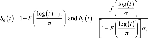
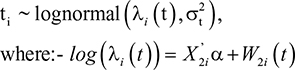
where S₀(t) is baseline survival, h₀(t) is baseline hazard rate, f(x) is normal density function; F(x) is cumulative normal density function, and μ and σ are model parameters. The survival time for the i^th subject follows the lognormal distribution,

(4)

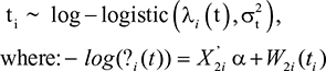
Second, in the log-logistic model, we assume that the survival time for the i^th subject follows a log-logistic distribution,

(5)

Third, we assume that the survival time for the i^th subject follows a Weibull distribution. Suppose the survival time T has Weibull distribution with scale parameter λ_i(t) and shape parameter k. Then under AFT model, the survival time T_i of the i^th individual is distributed as

(6)

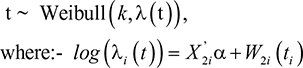
The Weibull distribution is used frequently in modeling survival and failure time data. It is known that its hazard function has monotonic behavior. However, when a hazard function is suspected to be nonmonotonic, log-logistic and lognormal distributions are useful alternatives. Log-logistic and lognormal distributions have hazard functions that each reach a peak and then decline over a period of time.^9,10

Joint model

In this study, the linear mixed effects model for the longitudinal process in Equation 1 and the AFT model for the time-to-event data in Equation 2 are linked assuming certain association between them. We assume that there is a stochastic dependence between the two models through the random effects W_1i and W_2i as follows:

(7)

(8)

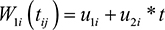
The parameter r measures the association between the two submodels, Equations 1 and 2, which is induced by the longitudinal term to the event time model. The latent u_1i variables u_2i and are independent subject-specific bivariate Gaussian random effects with mean zeros and constant variance. We call this scenario I.

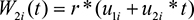
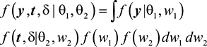
We consider scenario II by taking same W_1i (t) but W_2i (t) to be:

(9)

where the parameters r₁ and r₂ measure association between the two submodels induced by the random intercepts and slopes. A linear mixed effects model for longitudinal process includes subject-specific heterogeneous variance, with each patient receiving random intercept and linear slope terms, the longitudinal term at event time.¹¹

Bayesian joint model

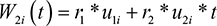
Using the usual joint modeling assumptions, subject-specific latent variables induce all the association between longitudinal process Y and survival time T. Therefore, if Y and T are conditionally independent given random effects W_i and denoting the model parameters by θ = {θ₁, θ₂}, then the full joint density function of the two processes is given as:

(10)

The respective likelihood function of interest is given as:

(11)

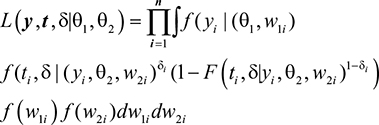
where θ₁ = {β, σ²_CD4, σ²_u} are the population parameters in the linear mixed effects model, θ₂ = {α, σ²_t, r} are the population parameters in the survival model, β is regression parameters in the mixed effects model, σ²_CD4 is the variance of the transformed CD4 cell count, σ²_u is the variance of subject-specific random error, a is regression coefficients in AFT model, σ²_t is the variance r of the transformed event time, r is the association parameters, f (.) and F(.) are probability density and distribution functions, respectively.

Noninformative prior distribution of the parameters are considered: β′s and α′s are normally distributed with mean zero and large variance 1,000, ie, small precision 0.001; association parameters r, r₁, r₂ are each assumed to have normal distribution with mean zero and variance 1,000, ie, small precision 0.001; the shape parameter k in Weibull and log-logistic distributions follows Gamma (2,0.5); all precisions parameters follow Gamma (2,0.5).

The joint posterior distribution for all model parameters q and random effects W are given by:

(12)

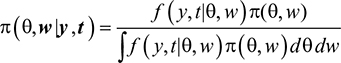
where π(θ,w/y, t) is posterior probability distribution, f(y, t/θ, w) is likelihood function, and π(θ,w) is prior probability distribution. Inference is based on Markov Chain Monte Carlo, which is Gibbs sampler and implemented in WinBUGS and R software.

Model selection

In this study, we compared three AFT models: lognormal, log-logistic, and Weibull probability distributions with separate and Bayesian joint approaches. The model selection procedure was based on the deviance information criteria (DIC), Akaike information criteria (AIC), and Bayesian information criteria (BIC). The DIC provides an assessment of model fitness and a penalty for model complexity. The DIC is a Bayesian alternative to the other two criteria.^12,13 It measures how best the selected model can predict future observations, given that it best fits to the data at hand.

DIC involves posterior mean that takes into account prior information and penalized likelihood. It is computed as:

(13)

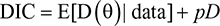
where D(θ) = –2log (Likelihood (θ/data)) is deviance, E[D(θ) | data] is the posterior mean of the deviance, and pD is effective number of parameters. AIC and BIC are computed as follows:

(14)

(15)

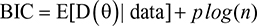
where p is the number of parameters in the model and n is the sample size. The models used in this study involve random effects and so DIC is more relevant for the model selection.

Results and discussion

The study considered 550 HIV/AIDS patients under ART follow-up. Among these, 58.5% are females and 41.5% males. For the longitudinal data, the average number of baseline CD4 counts was 162.47 per mm³ of blood with SD of 102.51. The results of the analysis showed that from the 550 patients included in the study, about 24.4% of them were dead, while 75.6% were censored, 65.1% of the patients has less than 200 CD4 count at baseline, and 34.9% were greater than or equal to 200 CD4 counts at baseline. About 67.3% are in working, 28.5% in ambulatory, and 4.2% in bedridden functional status. Regarding WHO disease stage, 14.9%, 32.7%, 42.5%, and 9.8% of them are, respectively, in stage 1, stage 2, stage 3, and stage 4. To check whether the PH assumption was violated or not, the corresponding P-value associated with a global test of nonproportionality is tested for the data set. The global test suggested strong evidence of nonproportionality (P<0.002), awareness about ART (P<0.015), and weight (P<0.035).

The simulations of the posterior distributions are made based on the Gibbs sampler with 60,000 iterations and three different initial states of the parameters with a burn-in of 20,000 iterations considered to be sure of convergence of all the simulations. Inferences are made based on independent samples taken after convergence of the realization. Time series plots, autocorrelations, and Gelman–Rubin statistics are assessed, and they all confirm convergences.

Scenario I

The joint models are linked through two random effects W_1i = u_1i + u_2i * t for longitudinal and W_2i = r * W_1i for time-to-event data. The prior distributions used for the regression parameters β and α are assumed to be random variables and having normal distributions with mean zero and constant variance. The posterior means and 95% CI of coverage probabilities, standard deviations of all separate and joint models are computed and displayed in Table 1.

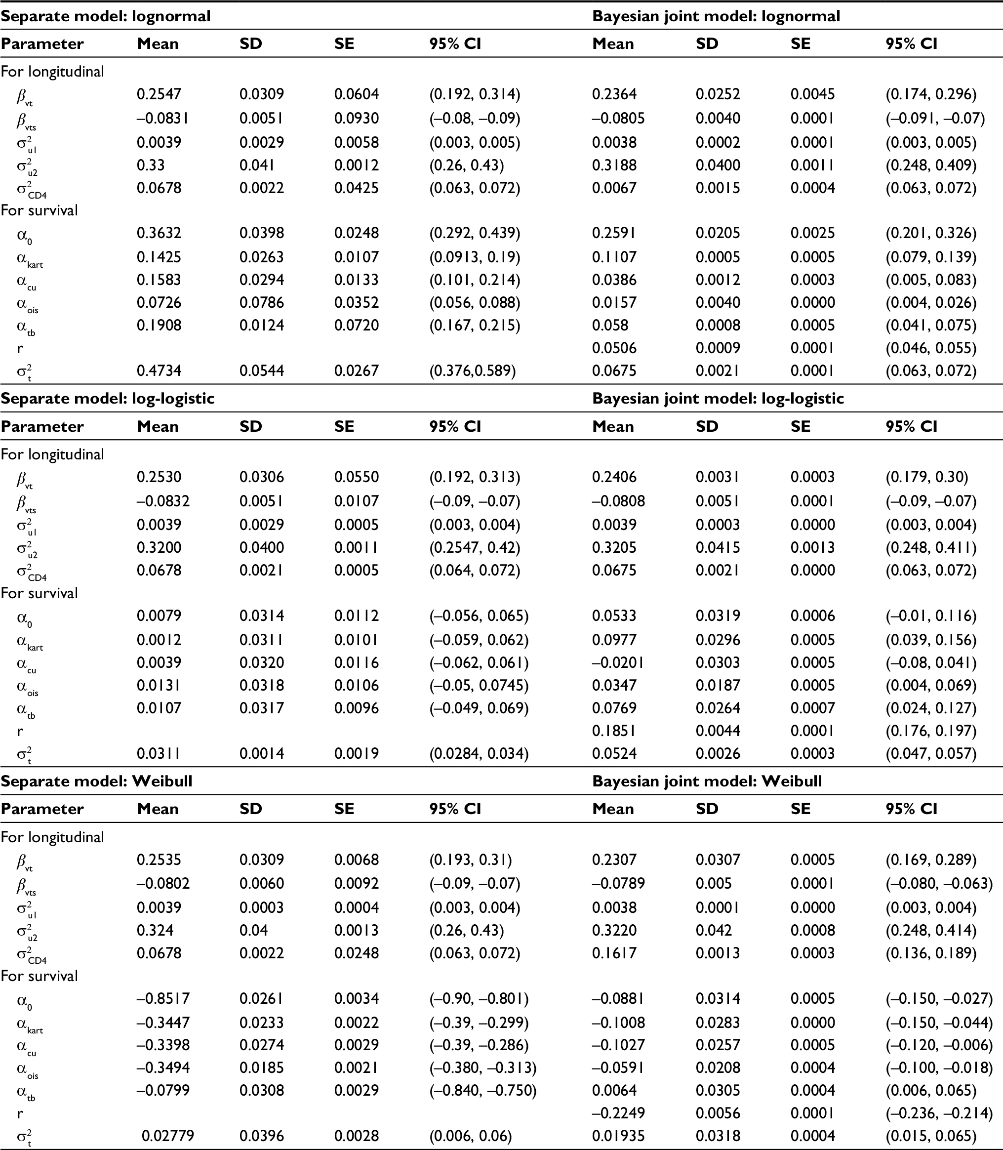Table 1 Posterior point estimates of separate and joint models in scenario I

From the Bayesian joint model analysis, the association parameter r is estimated to be r ̂ = 0.0506 for lognormal; r̂ = 0.1851 for log-logistic, and r ̂ = –0.2249 for Weibull cases. The 95% credible intervals for the association parameter r indicate that there is dependence between longitudinal term CD4 cell counts and time-to-event. The analysis gains power by the use of the Bayesian joint model.

The joint model allows borrowing strength between the CD4 cell counts data and the time-to-event data, in contrast to the separate models which often have standard errors of larger magnitude. Bayesian joint models provide estimates of all parameters with smaller posterior standard errors.

The significant predictors in each of the three Bayesian joint models are found to be visit time (vt), visit time square (vts), association coefficient (r), and knowledge about ART (kart), opportunistic infection (ois), condom use (cu), and TB status (tb). They are all statistically significant as seen from the 95% credible intervals that do not contain zero. The estimated average regression coefficients of visit time for the longitudinal outcome are 0.2364, 0.2406, and 0.2307 for lognormal, log-logistic, and Weibull models, respectively. The positive sign suggests significant increase in CD4 cell count over the study period. But the estimated parameter of the square of visit time is negative. This possibly indicates a nonmonotone effect of visit time on CD4 cell counts.

The estimated association parameter in the Bayesian joint models of log-normal and log-logistic is positive. But in case of Bayesian joint model of Weibull, the association parameter is negative. The negative estimates of r for the Weibull case correspond to the fact that the model has a monotone hazard rate function, while the data reveal a nonmonotone hazard. Moreover, the parameter point estimates of the Bayesian joint models are similar to those of the separate models, indicating certain coherence.

Scenario II

In this case, the random effects are W_1i = u_1i + u_2i * t for the longitudinal and W_2i = r₁ * u_1i + r₂ * u_2i for the time-to-event component. Prior distributions used for the parameters r, r₁, r₂, β_i and α₁ are normally distributed with mean zero and large variance 1,000 and σ_i² ~ Gamma(2,0.5). The posterior means and 95% credible intervals, standard deviation of the both the separated and the joint models are estimated and displayed in Table 2.

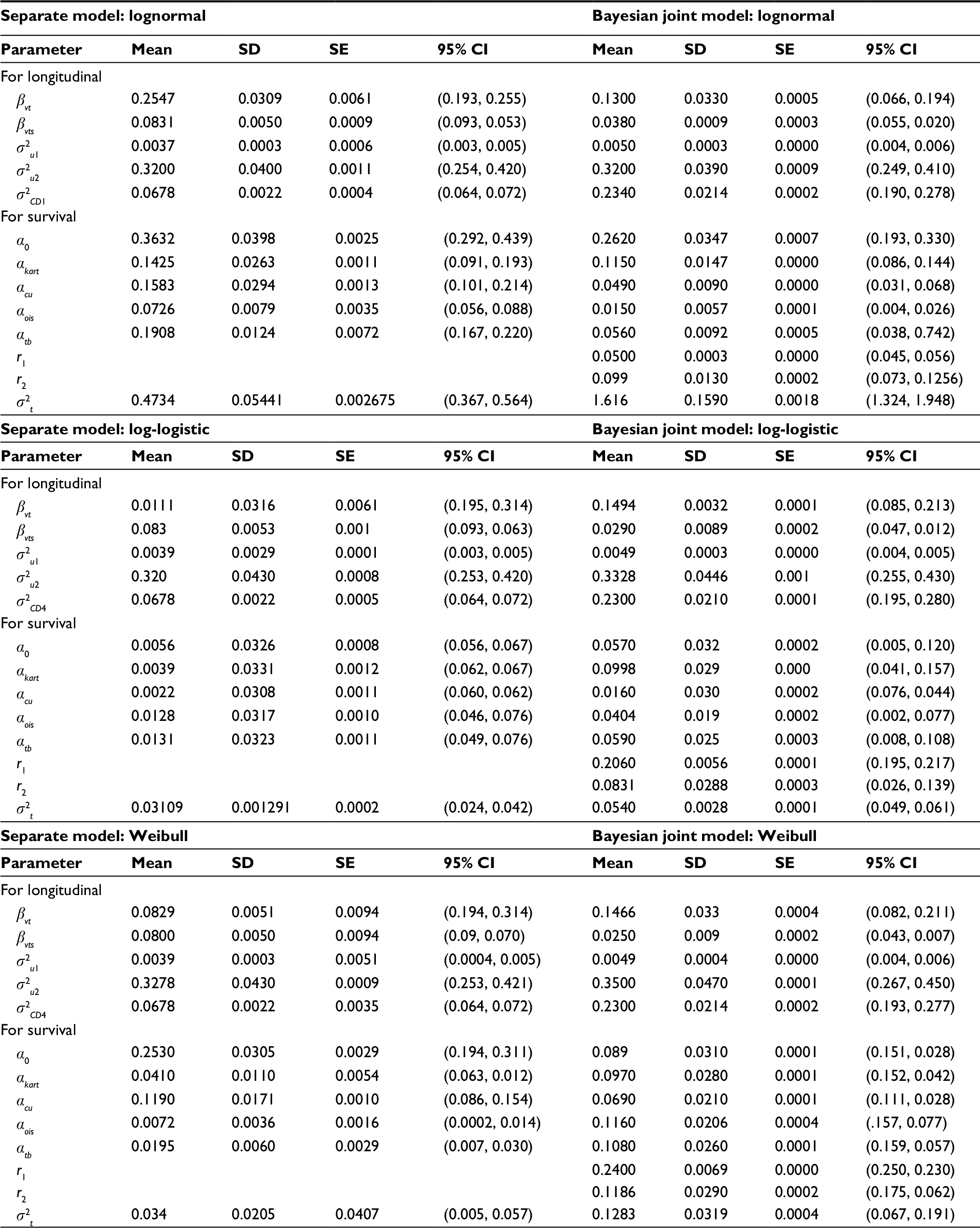Table 2 Posterior point estimates of separate and joint models in case of scenario II

Table 2 shows that r1 and r2 are significantly different from zero. This shows that there is an association between the longitudinal and time-to-event models induced by the random intercepts and slopes. As before, the parameters are estimated with smaller bias in the joint models with respect to the two models separately. The posterior estimates of the association parameters in the joint analysis with the Weibull distribution are also negative like scenario I. The negative sign indicates that both the initial level and the slope of CD4 cells count are negatively associated with the hazard rate of death. The posterior estimates of the association parameters are positive for the joint analysis with lognormal and log-logistic distributions. But it is negative for joint analysis of Weibull. This difference might be due to the nonmonotonic hazard rate of the lognormal and log-logistic models compared with the monotonic hazard rate of the Weibull submodel. The empirical hazard rate estimates in Figure 1 shows nonmonotonicity, showing the suitability of log-logistic and lognormal models rather than the Weibull model for modeling our failure time data.

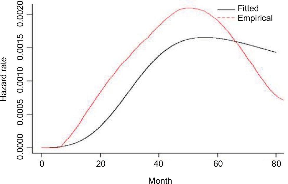Figure 1 Empirical and fitted hazard rate estimates.

Already Bennett recommended using the log-logistic distribution for modeling hazards peaking after some time and then slowly declining.¹⁰ In most of HIV/AIDS studies, the hazard rate or the mortality rate decreases or increases but only in few studies the hazard rate function increases up to peak point and then declines slowly. For instance, Byers et al estimate HIV/AIDS infection rate in the San Francisco cohort, and the hazard rate function reaches a peak at 27.6 months and then declines slowly.¹⁴ The investigators found that the estimated hazard rate functions for one treatment were increasing, while it was increasing-and-then-decreasing over time for the other treatments. Laurent et al,¹⁵ Severe et al,¹⁶ and Braitstein et al¹⁷ found that in resource-poor countries access to ART has improved during the last few years and mortality rates among treated patients have declined significantly. However, compared with patients in high-income countries, patients in resource-poor countries are at higher risk of death in the early months of treatment. This may indicate that the hazard rate in developing countries increases and then slowly declines after reaching a peak point. According to Andinet and Miguel,¹⁸ the mortality rates increase in the first few months of therapy and then slowly decrease in different African countries, including Ethiopia.

Study from South Africa on early mortality and access to antiretroviral serves clearly indicate the risk of death to be independently associated with low baseline CD4 cell count and WHO stage IV with majorly attributed causes of death to be TB, acute bacterial infections, and failure to immune reconstitution.¹⁹ Similarly a study by Asfaw et al from Ethiopia, indicate that CD4 cells depletion prior to ART start found to be consistently most determinants for ensuing increase in CD4 cells count after ART start thereby immune reconstitution.²⁰ The investigators indicated low level of baseline CD4 cell count before ART initiation to have increased the risk of morbidity and mortality. This might be explained by the fact that very few immune cells will have hard time to tolerate toxicity of ART drugs to induce immunological boost to fight against cocktails of diseases due to their depletion.

In conclusion, the shape indicates diverse situations and a variety of shapes sometimes increasing or decreasing, and sometimes growing and then declining. Therefore, it is important to look at the empirical hazard function before deciding the appropriate time-to-event model.

We now compare our models formally; see Table 3 for both scenarios I and II; the estimated BIC and AIC for Bayesian joint models are smaller than respective separated models. The results indicate that the Bayesian joint models are better than the respective separate models.

Table 3 Model comparison of separate and joint models for both scenarios Abbreviations: Dbar, posterior mean of the deviance; AIC, Akaike information criteria; BIC, Bayesian information criteria; DIC, deviance information criteria.

Comparing the three distributions for the time-to-event component, see Table 4, we conclude that the Bayesian joint model with log-logistics is preferred than other models for HIV/AIDS data used in this study.

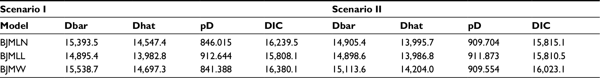Table 4 Result of model comparison of Bayesian joint models Abbreviations: Dbar, posterior mean of the deviance; Dhat, deviance of the posterior means; PD, effective number of parameters; DIC, deviance information criteria; BJMLN, Bayesian Joint Model of Lognormal; BJMLL, Bayesian Joint Model of Log-Logistic; BJMW, Bayesian Joint Model of Weibull.

Based on above analysis, we conclude that the Gibbs sampler for the Bayesian joint model with lognormal, log-logistic, and the Weibull distributions converges well.

Conclusion

The objective of this study was to compare separate models and joint models for longitudinal and survival data set. AFT is useful when the assumption of PH fails to be true, like in our case. The results indicate that linear visit time and squared visit time were statistical significant for the longitudinal CD4 cells count, knowledge about ART, condom use, TB infection status, and opportunistic infections were significant in the time-to-death model.

When evaluating the overall performance of the separate vs the joint models, the Bayesian joint model performs better. When comparing the fitted of all the three AFT distributions in the Bayesian joint models, we find that the log-logistic distribution fits our data best.

We model the link between the AFT and the longitudinal component in two different ways, with one parameter r in the first case and two parameters r1 and r2 in the second case. Association coefficients r, r1, and r2 are all significantly different from zero; this implies that there is dependence between the longitudinal and time-to-event data.

The posterior estimates of these association parameters in the joint analysis with the Weibull distribution are negative compared with all other models. This is due to the nonmonotonicity of the hazard rate in our data. We recommend inspecting the empirical hazard rate and if it is not monotone to use the log-logistic or the lognormal models instead of the Weibull modeling for modeling failure time data.

Acknowledgments

The authors thank the anonymous reviewers for their comments that were useful to improve the write-up of the paper and Arba Minch General Hospital for providing the data sets used in this study.

Disclosure

The author reports no conflicts of interest in this work.

References

1.		Henderson R, Diggle P, Dobson A. Joint modeling of longitudinal measurements and event time data. Biostatistics. 2000;4:465–480.
2.		Wu L, Liu W, Yi GY, Huang Y. Analysis of longitudinal and survival data: joint modeling, inference methods, and issues. J Probab Stat. 2012;2012(3):1–17.
3.		Tsiatis AA, Davidian M. Joint modeling of longitudinal and time-to-event data: An overview. Stat Sin. 2004;14(3):809–834.
4.		Yu M, Law NJ, Taylor JM, Sandler HM. Joint longitudinal-survival-cure models and their application to prostate cancer. Stat Sin. 2004;14(3):835–862.
5.		Tseng Y-K, Hsieh F, Wang J-L. Joint modelling of accelerated failure time and longitudinal data. Biometrika. 2005;92(3):587–603.
6.		Hatfield LA, Hodges JS, Carlin BP. Joint models: When are treatment estimates improved? Statistics and Its Interface. 2014;7(4):439–453.
7.		Zhou J, Zhao X, Sun L. A new inference approach for joint models of longitudinal data with informative observation and censoring times. Stat Sin. 2013;23:571–593.
8.		Guo X, Carlin BP. Separate and joint modeling of longitudinal and event time data using standard computer packages. Am Stat. 2004;58(1):16–24.
9.		Farewell VT, Prentice RL. A study of distribution shape in life testing. Technometerics. 1979;19:69–75.
10.		Bennett S. Log-logistic regression models for survival data. Appl Stat. 1983;32(2):165–171.
11.		Guo X, Carlin BP. Separate and joint modeling of longitudinal and event time data using standard computer packages. Am Stat. 2004;58(1):16–24.
12.		Robert CP. The Bayesian Choice: From Decision-Theoretic Foundations to Computational Implementation. 2nd ed. Springer LLC; 2007:373–376.
13.		Spiegelhalter D, Thomas A, Best N, Lunn D. WinBUGS Version 1.4 User Manual; 2003. Available from: http://www.mrc-bsu.cam.ac.uk/bugs/winbugs/manual14.pdf. Accessed January, 2003.
14.		Byers RH, Morgan WM, Darrow WW, et al. Estimating AIDS infection rates in the San Francisco cohort. AIDS. 1988;2(3):207–210.
15.		Laurent C, Ngom Gueye NF, Ndour CT, et al. Long-term benefits of highly active antiretroviral therapy in Senegalese HIV-1-infected adults. J Acquir Immune Defic Syndr. 2005;38(1):14–17.
16.		Severe P, Leger P, Charles M, et al. Antiretroviral therapy in a thousand patients with AIDS in Haiti. N Engl J Med. 2005;353(22):2325–2334.
17.		Braitstein P, Brinkhof MW, Dabis F, et al. Mortality of HIV-1-infected patients in the first year of antiretroviral therapy: comparison between low-income and high-income countries. Lancet. 2006;367(9513):817–824.
18.		Andinet W, Miguel S. Determinants of survival in adult HIV patients on antiretroviral therapy in Oromia, Ethiopia. Open Access article. Global Health Action. 2010;3:5398.
19.		Lawn SD, Myer L, Orrell C, Bekker LG, Wood R. Early mortality among adults accessing a community-based antiretroviral service in South Africa: implications for programme design. AIDS. 2005;19(18):2141–2148.
20.		Asfaw A, Ali D, Eticha T, Alemayehu A, Alemayehu M, Kindeya F. CD4 cell count trends after commencement of antiretroviral therapy among HIV-infected patients in Tigray, Northern Ethiopia: a retrospective cross-sectional study. PLoS One. 2015;10(3):e0122583.