Analysis of severity of childhood anemia in Malawi: a Bayesian ordered categories model

Introduction

Infant anemia is a global public health problem. According to the World Health Organization’s most recent report on the world prevalence of anemia,¹ the global prevalence of anemia is 24.8% with the highest prevalence in the sub-Saharan Africa (67%), followed by the Southeast Asia (65.5%). Preschool-aged children are reported to have the highest prevalence (47.4%); however, estimates from a systematic review report² suggest that the world prevalence of anemia for this population group has slightly decreased from 47% to 43%, with the South Asia, Central Africa, and West Africa still having the highest prevalence. Malawi alone, as part of the sub-Saharan Africa, has 63% prevalence of childhood anemia, according to the 2010 Malawi Demographic and Health Survey (MDHS) report.³

Consequences of childhood anemia are poor cognitive development for mild and moderate anemia and death for severe anemia. Severe anemia carries a significant risk of death by profound hypoxia and congestive heart failure or, more rarely, by cerebral malaria.^4,5

The prevalence of anemia is influenced by a number of factors. It is said that 50% of all anemia cases are due to iron deficiency.⁶ Anemia is also due to the deficiency of other micronutrients such as vitamin A, vitamin C, and folate. Diseases such as malaria, human immunodeficiency virus, bacteremia, and helminth infections caused by hookworm and Schistosoma haematobium are also known to influence anemia.^7,8 Infections lead to anemia through blood loss, hemolysis by antibodies, and anemia of inflammation. Furthermore, previous studies have also shown that low parental education levels, low household income, and demographic factors such as age, sex, and family size affect anemia.^9–11 Sickle-cell disease has also been documented as a risk factor for anemia in sub-Saharan countries.¹²

Most studies on childhood anemia have used binary logistic regression and linear regression to investigate factors that influence childhood anemia. For example, many studies^11,13–15 use a binary logistic model and some^9,10 use a Gaussian model. A binary logistic model is used when childhood anemia as a response is binary (non-anemic [hemoglobin {Hb} ≥11 g/dL] or anemic [Hb <11 g/dL]), and a Gaussian model is used when childhood anemia as a response is a continuous measure of Hb level. Nevertheless, the interest in analyzing the severity of the disease and the corresponding risk factors is of epidemiological importance.^16–18 In cases where childhood anemia can be considered as an ordered response (ie, nonanemia [Hb ≥11 g/dL], mild anemia [10.0 g/dL ≤ Hb ≤ 10.9 g/dL], moderate anemia [7.0 g/dL ≤ Hb ≤9.9 g/dL], and severe anemia [Hb <7.0 g/dL]), a multinomial ordered model is appropriate. To our knowledge, a few studies though have employed the use of multinomial ordered outcome model for childhood anemia.^16–18 The use of a multinomial ordered outcome model may help identify children at the greatest risk to anemia, which is important when resources are inadequate.

This study aims at investigating factors of childhood anemia in Malawi by using multinomial ordered outcome model, extended to permit nonlinear effects of some continuous variables and spatial effects of district of residence. Spatial effects are surrogates of unknown influences, eg, climatic and environmental factors, access to good transport system, and access to good child health care services. These unknown factors may have a localized effect (uncorrelated/unstructured) or global effect (correlated/structured). Mapping geographical spatial effects to childhood anemia severity would have important implications to policy.

The paper is organized as follows: first, the “Patients and methods” section in terms of study population, area, data, and statistical analysis is presented. It is followed by the “Results”, “Discussion”, and “Conclusion” sections.

Patients and methods

Study area and data

The study focused on children <5 years old in Malawi and used the standard and nationally representative 2010 MDHS data. The 2010 MDHS was conducted from June 2010 to November 2010. Data were downloaded from the DHS web site (www.dhsprogram.com/data/dataset_admin) after being granted permission. Parents of the patients signed informed consent. The Malawi Health Research Committee saw that ethical approval was not deemed necessary in this study considering the fact that the study used data from a research study already approved by an ethical research committee. According to the 2010 MDHS report,³ the 2010 MDHS study was ethically approved by Malawi Health Research Committee, Institutional Review Board of ICF Macro, Centre for Disease and Control (CDC) in Atlanta, GA, USA. Furthermore, mothers whose children were tested for anemia, voluntarily allowed their children to be tested. The sampling design according to the 2010 MDHS report³ was a two-stage cluster design with stratification. The primary sampling units were the enumeration areas (EAs), and the secondary sampling units were the households. EAs were stratified in terms of rural and urban. A total of 849 EAs were sampled with 158 in urban areas and 691 in rural areas. A total representative sample of 27,307 households was selected, and 25,311 households were considered to be occupied in the 2010 MDHS. Data collection was done through questionnaires. There were three types of questionnaires: woman, man, and household questionnaires, and data were collected through face-to-face interviews also. Total households that were successfully interviewed were 24,825, yielding a response rate of 98%. Out of 23,748 eligible women, 23,020 were successfully interviewed, yielding a response rate of 97%. Out of 7,783 eligible men, 7,175 were successfully interviewed, yielding a response rate of 92%. The data set used in the analysis was child record data set, which was based on woman and household questionnaires.

Data management in terms of extracting and generation of variables from child record data set was done in STATA Version 12 (StataCorp, College Station, TX, USA). Data variables used in this study were based on the variables used in previous studies on childhood anemia.^8–10 The response variable in the extracted data set was child anemia status, which was grouped into four categories that are defined as follows:

• Category 1: non-anemia (Hb ≥11 g/dL)
• Category 2: mild anemia (10.0 g/dL ≤ Hb ≤ 10.9 g/dL)
• Category 3: moderate anemia (7.0 g/dL ≤ Hb ≤ 9.9 g/dL)
• Category 4: severe anemia (Hb <7.0 g/dL).

The four categories for child anemia status are based on categorization of child hemoglobin level using cutoff points according to World Health Organization.¹⁹ The covariates in the generated data set were mother education level (no education, primary, secondary, and higher), family wealth index (poorest, poor, rich, richer, and richest), child cough (yes/no), child fever (yes/no), receiving vitamin A (yes/no), stunting (height for age z-score [HAZ] <−2/HAZ ≥−2), wasting (weight for height z-score [WHZ] <−2/WHZ ≥−2), underweight (weight for age z-score [WAZ] <−2/WAZ ≥−2), childbirth weight in kilograms, childbirth order (1, 2–3, 4–5, 6+), household size (≤5/>5), child’s age in months, mother’s age in years, breast-feeding in months, and district of the child. Child’s age in months, mother’s age in years, and the breast-feeding in months were continuous covariates. District of residence of child i was denoted as s_i ∈ (1, 2, 3, …, S), corresponding to the label on the map. All children records where childhood anemia status was missing were dropped so that the final sample size of children in terms of the response was 4,177, representing 81% of children in the original sample.

Statistical model

A common tool for analyzing regression data with ordinal responses is the cumulative threshold model.²⁰ The model assumes that the response variable Y, here child anemia status, is a categorized version of a latent continuous variable, say in this study, child Hb level.

where η is the predictor of the latent variable, and U and ε are the error variables. The two variables Y and U are linked by Y = r if and only if θ_r−1<U<θ_r, r = 1, 2, 3, …, k with thresholds ∞ = θ₀ < θ₁ … <θ_k = ∞. Here r = 1, 2, 3, …, k are the categories of the variable Y based on the range of the latent variable U, and the thetas, θ_r, are the boundaries for these categories. For example, suppose r = 4, as it is the case in this study, then θ₁ demarcates category 1 from category 2, θ₂ demarcates category 2 from category 3, and θ₃ demarcates category 3 from category 4. It follows immediately that Y is determined by the model Pr(Y≤r) = F(θ_r−η) so that

where F⁻¹ is the link function. If the errors have the standard normal distribution, ie, N(0,1), then the link function F⁻¹ is the probit link so that Equation 2 is the probit model, and if the errors have the extreme value distribution, then the link function is the complimentary log–log, which makes Equation 2 to be the proportional hazard model. If the errors have the logistic distribution, then the link function is logit link so that Equation 2 is the cumulative logit model. In this study, we assumed errors to be distributed as logistic so as to have the cumulative logit model.

The basic assumption of course is that the predictor η in Equation 2 is linear. To take a more flexible approach, the continuous covariates and the area level random effects were modeled by the nonlinear smooth functions. This assisted in revealing their subtle influences, which could not be shown if modeled linearly. To reflect this flexible approach, the predictor in the cumulative logit model (Equation 2) was extended as follows:

where f_j for j = 1, 2, 3, …, p are smooth functions expressing nonlinear relationship between the response variable and the continuous covariate, and f_spat (s_i) is the area of the child random effect. The vector of coefficients γ determines the parametric relationship between the response and the categorical covariates. The smooth functions f_j were specified as Bayesian splines. According to Fahrmeir and Tutz,²⁰ this assumes approximating f_j by the polynomial spline of degree l defined at equally spaced knots , which are within the domain of the covariate x_j. The Bayesian spline can be written as a linear combination of d = s+1 basis functions, B_m, ie,

According to Ruppert,²¹ the number of knots d should be large enough from 5 to 20 to ensure more flexibility, while Eilers and Marx²² say that the number of knots must be between 20 and 40. In this study, the number of knots for each f_j was specified to be 20. Now Bayesian estimation of the penalized spline (Equation 4) is equivalent in estimating model parameters ε_j = (ε_j1, ε_j2, …, ε_jm), where the first- or second-order random walk priors for the regression coefficients are assigned. A first-order random walk prior for equidistant knots is given by ε_jm= (ε_j,m−1 + u_j,m), where m = 2, 3, …, d, and a second-order random walk prior for equidistant knots is given by ε_jm = 2ε_j,m−1 + ε_j,m−2 + u_j,m, where m = 3, 4, …, d and are random errors. The spatial effect was modeled by the tensor product of two-dimensional spline defined as

where (x₁, x₂) refers to the coordinates of the location of the data point, latitude and longitude, or location centroids based on the map. Note that f_spat (x₁, x₂) represents the effect of correlated unmeasured or unobserved location effects. The prior for B_spat,ij = (B_spat,11, B_spat,12, …, B_spat,kk) is based on spatial smoothness priors common in spatial statistics.²³ The most commonly used prior specification based on the four nearest neighbors is defined as

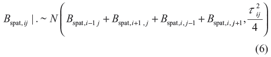
for i, j = 2, …, k − 1 with appropriate changes for corners and edges. Model inference was by empirical Bayesian approach via mixed model methodology. This was implemented in BayesX, a program for Bayesian inference in combination with R (R Core Team, Austria). Some of the R code for model fitting is in the Supplementary material section. Since model estimation was by empirical Bayesian method, all variance parameters were treated as unknown constants that were estimated by restricted maximum-likelihood method, and hence, their priors were not given. The fixed effects were assigned diffuse priors. An advantage of the empirical Bayesian inference over full Bayesian inference is that questions about the convergence of MCMC samples or sensitivity on hyper parameters do not arise.²⁴

Results

Descriptive summaries

Table 1 shows the prevalence of childhood anemia by some of the covariates. It is observed that 23% of the children have mild anemia, 36% have moderate anemia, and 3% have severe anemia. The prevalence of anemia is highest among children aged 6–11 months and decreases with age between 12 and 59 months (χ²=336.92, P<0.001). Fifty three percent of children in urban areas have anemia, compared with 64% of children in rural areas (χ²=20.28, P<0.001). Childhood anemia decreases with an increase in mother education (χ²=22.97, P=0.006) and with wealth quintile (χ²=60.87, P<0.001). There is also regional difference in childhood anemia with the northern region having slightly lower prevalence (58%) than the central and southern regions (64% and 62%, respectively) (Table 2). The Pearson’s chi-squared test of association between region and childhood anemia supports this observation as P-value for the chi-square test is <0.05.

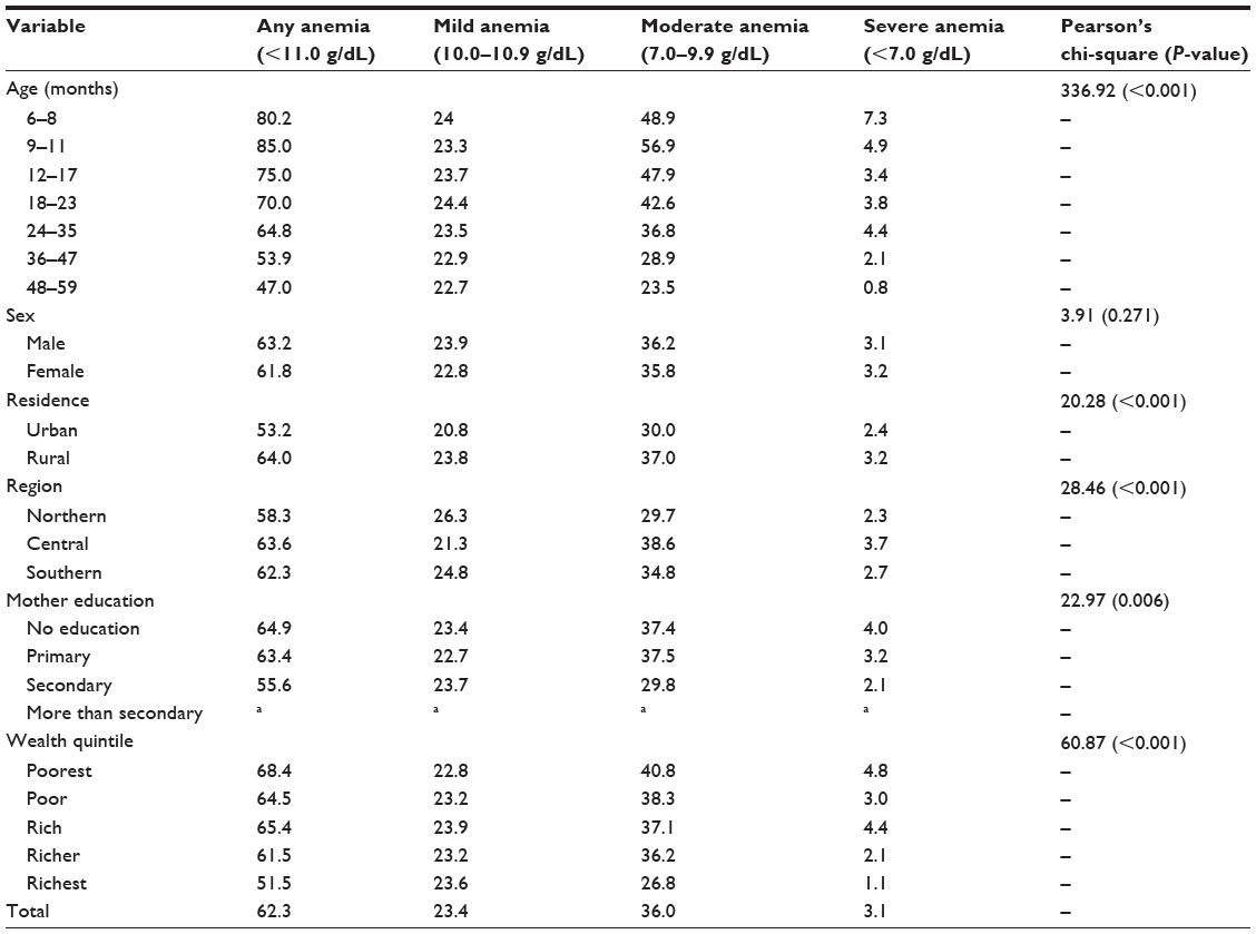Table 1 Percentage of childhood anemia per some covariates and bivariate Pearson’s chi-squared test Notes: aIndicates that a figure is based on <25 unweighted cases and has been suppressed. – Not applicable.

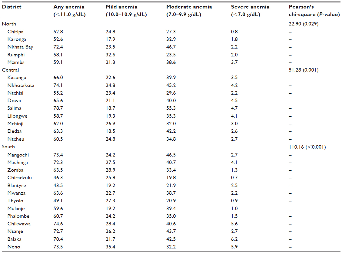Table 2 District percentage distribution of childhood anemia status and bivariate Pearson’s chi-squared test Note: – Not applicable.

Empirical Bayesian

Testing proportional odds assumption of cumulative logit model

To have a meaningful interpretation of results from the cumulative logit model, the validity of proportional odds assumption was first tested. Table 3 presents the results of this test. The assumption of proportional odds for the cumulative logit model was not violated as the likelihood ratio chi-square P-value for the difference in log-likelihood between the full multinomial logit model (results not tabled) and the full cumulative logit model (Table 4, Model 4) was >0.05. Thus, the results of the cumulative logit model could then be further presented and interpreted.

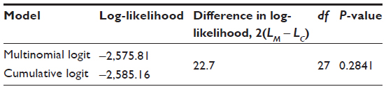Table 3 Testing proportional odds assumption Abbreviations: df, degrees of freedom; M, multinomial logit; C, cumulative logit.

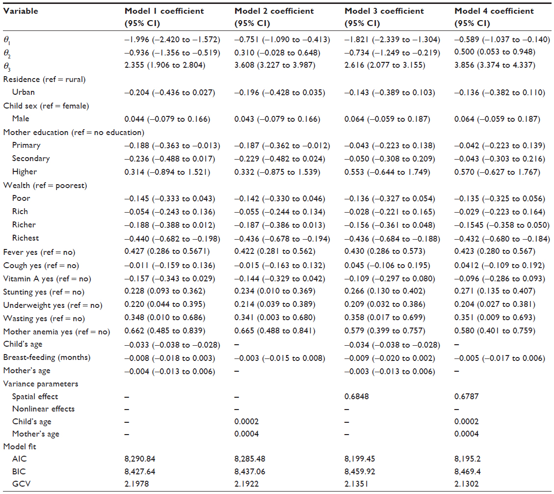Table 4 Summary of four cumulative logit models Notes: Model 1 (fixed effects), Model 2 (fixed plus nonlinear effects), Model 3 (fixed and spatial effects), and Model 4 (geoadditive). – Not applicable. Abbreviations: CI, credible interval; AIC, Akaike information criterion; BIC, Bayesian information criterion; GCV, generalized cross-validation; ref, reference.

Model selection

A number of models were fitted. Model 1 was a fixed-effects model, while Model 2 had linear and the nonlinear effects. In Model 3, all covariates were modeled as fixed effects, except district of residence, which was random. In the last model, Model 4, in addition to the fixed effects, it captured the nonlinear effects of some continuous covariates and the random effect of district of the child. Model selection is by the use of Akaike information criterion (AIC), Bayesian information criterion (BIC), and generalized cross-validation (GCV) as used by Kneib et al²⁵ when they used empirical Bayesian method in the estimation of the structured additive regression model. A model with the smallest AIC, BIC, or GCV is considered as the best model. BIC tends to give a larger penalty to overfitting than the AIC and hence tends to select simpler models. The GCV does not give any penalty to overfitting, and it tends to select more fitting models. Table 4 shows that AIC and GCV favor Model 4 and BIC favors Model 1. Therefore, the discussion of the results is based on the geoadditive model (Model 4) selected by both AIC and GCV.

Fixed effects

The cutoff point between non-anemia and mild anemia is θ₁, the cutoff point between mild and moderate anemia is θ₂, and the cutoff point between moderate and severe anemia is θ₃. The sign of these cutoff point parameters means a shift toward an area of low or high probability with regard to probability distribution of the latent variable. Table 4 shows that the threshold parameter for category “non-anemia” (θ₁) is negative, which means having non-anemia corresponds to reduced probability of having anemia. Also the negative sign for the threshold parameter of “mild anemia” (θ₂) means that mild anemia category is associated with reduced probability of having anemia. The positive sign for the threshold parameter for “moderate anemia” (θ₃) means that moderate anemia category is associated with increased probability of having anemia.

The sign of the covariate coefficient means being associated with higher or lower levels of childhood anemia on the childhood anemia category rating scale compared to the baseline. In Table 4, the fixed-effects variables found significant to childhood anemia are fever, wealthy family of richest category, stunting, wasting, underweight, and mother anemia status. The coefficient of fever (0.423; 95% credible interval [CI]: 0.280−0.567) is positive, which means that fever is associated with higher levels of childhood anemia, severe anemia, eg, compared to having no fever. The richest family has a negative effect on childhood anemia severity, that is, the children of the richest family are associated with less anemia compared to the children of the poorest family. The coefficient for stunting (0.271; 95% CI: 0.135−0.407) is positive, which means that the stunted children are associated with severe childhood anemia compared to the nonstunted children. Similarly, the effect of underweight and wasting is positive, which means that the children who are underweight or wasted are associated with higher levels on childhood anemia rating scale, say severe anemia. Mother anemia status has a positive effect on childhood anemia (coefficient: 0.580; 95% CI: 0.401−0.759), which means that the children of anemic mothers are associated with severe childhood anemia compared to those whose mothers do not have anemia.

Nonlinear effects

Figure 1 presents the nonlinear effects of age of the child. As the child’s age increases, its effect on childhood anemia decreases, that is, older children are less likely to have childhood anemia. The chance of having anemia is much higher in children aged ~5 to ~20 months and decreases thereafter.

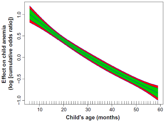Figure 1 Nonlinear effect of child’s age on childhood anemia. Note: Red band (95% CI) and green band (80% CI). Abbreviation: CI, credible interval.

With regard to mother’s age (Figure 2), there is a U functional relationship between childhood anemia and mother’s age. Young mothers are more likely to have children who are anemic, in particular, mothers aged 15–25 years. The risk of childhood anemia remains equal and is reduced for mothers aged 25–40 years. The risk of childhood anemia then rises for mothers who are aged 40 years and above.

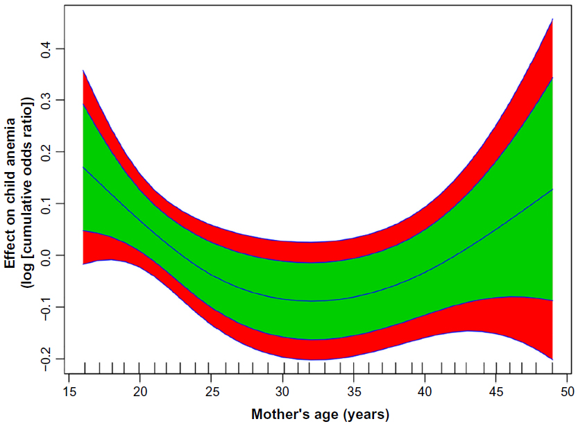Figure 2 Nonlinear effect of mother’s age on childhood anemia. Note: Red band (95% CI) and green band (80% CI). Abbreviation: CI, credible interval.

Spatial effects

Figure 3 presents total residual spatial effects on childhood anemia. Chikwawa, Salima, and Nkhotakota increase the probability of having severe childhood anemia, while Chiradzulu reduces the probability of severe childhood anemia at the 95% credible interval (Figure 4). For the 80% credible interval (Figure 5), Nkhotakota, Salima, Mangochi, Machinga, Balaka, Chikwawa, and Nsanje increase the probability of having severe anemia, and Chitipa, Karonga, Rumphi, Mzimba, Chiradzulu, and Thyolo reduce the probability of having severe childhood anemia.

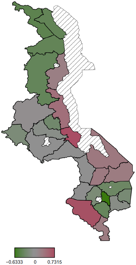Figure 3 Residual spatial effects on childhood anemia.

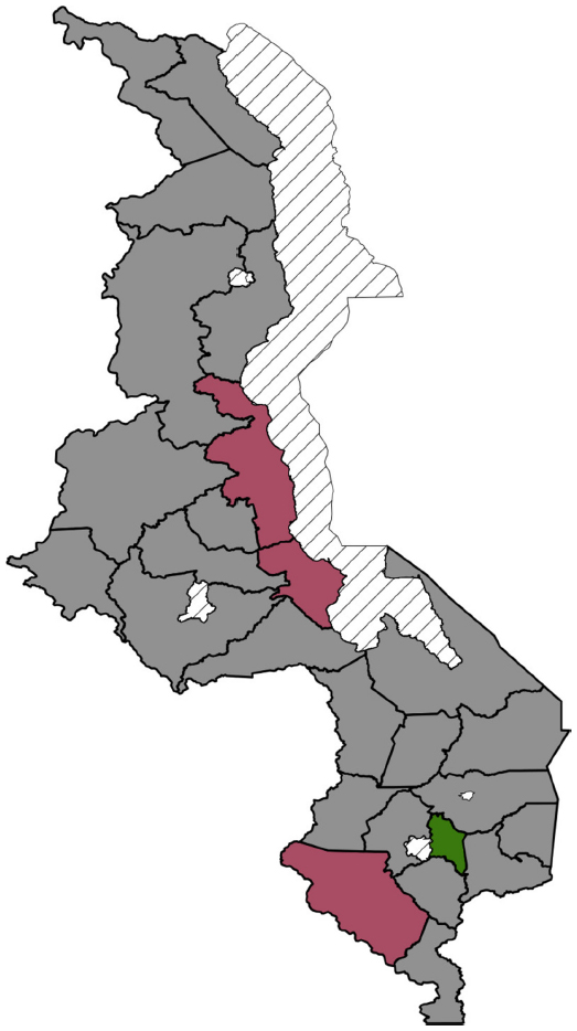Figure 4 The 95% posterior credible intervals map for the spatial effects. Note: Red means positive effect, green means negative effect, and gray means insignificant effect.

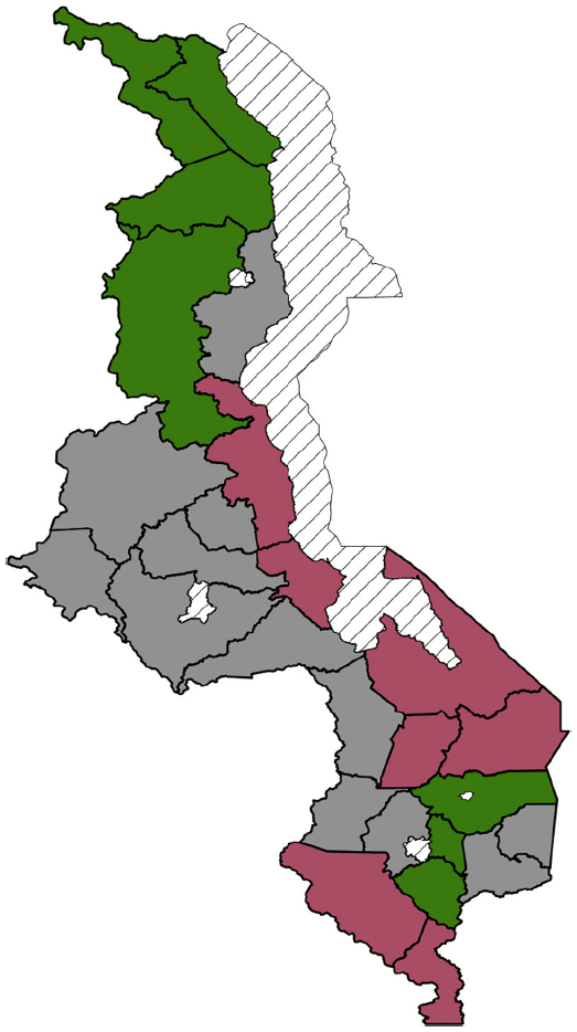Figure 5 The 80% posterior credible intervals map for the spatial effects. Note: Red means positive effect, green means negative effect, and gray means insignificant effect.

Discussion

This study employed the use of geoadditive multinomial ordered outcome model for childhood anemia, which allowed the identification of children who are at the greatest risk to anemia and the priority areas for action, especially where resources are inadequate. The geoadditive model allowed the mapping of residual spatial effects to childhood anemia while accounting for nonlinear covariate effects under the assumption of additivity. Modeling of metrical continuous covariates nonlinearly captured their subtle influences so that their effects could not be rejected if they were modeled linearly. For example, mother’s age was found to be insignificant when modeled as a fixed effect in Models 1 and 3 (Table 4) as its effective CI contained a zero but was found to have a nonlinear effect when modeled nonparametrically by a smooth function in Models 2 and 4 (Figure 1).

The incorporation of spatial effect in the models helped to avoid underestimating the standard errors of model parameters, thereby avoiding wrong statistical significance of covariates since their credible intervals would be narrower. For example, mother education and primary category coefficients were found to be significant in Models 1 and 2 where there was no spatial effect, but were not significant in Models 3 and 4 (Table 4) when the spatial effect was included in the models.

The observed spatial heterogeneity may be due to unobserved factors not captured by the covariates in the models, and it is a matter of conjecture to identify them. The geographical variation in anemia-causing infections, such as malaria, hookworms, and helminths, could be one influence of such spatial variation. Malaria is common in places near water bodies and where temperature is high (>21%). The optimum temperature for the development of mosquitoes is between 22°C and 32°C.²⁶ Soil moisture and relative atmospheric humidity are also known to influence the development and survival of ova and larvae for hookworms and helminths, where higher humidity is associated with faster development of ova.^27,28 Salima, Nkhotakota, Mangochi, Machinga, and Balaka were observed to have a high risk to anemia at 20% significance level probably due to closeness to Lake Malawi, Lake Malombe, Lake Chiuta, Lake Chilwa, and Shire River, which enhance the development of mosquitoes, hookworms, and helminths. The transmission of hookworms and helminths along such water bodies would also be facilitated by open fecal disposal according to Coffey²⁹ since along these water bodies, open fecal disposal is common, particularly by fishermen. Similarly, Nsanje and Chikwawa districts have a high risk to childhood anemia probably because they are characterized by permanent wetlands (Ndindi and Elephant marsh) with large stretches of stagnant water and their temperatures are >21°C, which provide the best ground for mosquitoes to breed, resulting in increased malarial transmission and let alone malaria anemia.

The height above the sea level (altitude) has another possible influence of spatial heterogeneity in anemia. Areas at higher altitudes are associated with higher Hb levels than those at lower altitudes. According to Rutstein and Rojas,³⁰ this difference is due to the lower oxygen concentration at higher altitude than at lower altitude so that an individual at high altitude requires relatively a large number of Hb cells to carry enough oxygen needed by the body. Highland areas also have lower temperatures and thus are associated with less risk to malaria anemia. Most areas in the north, such as Rumphi, Mzimba, Chitipa, and part of Karonga, are at a high altitude, and this may explain their reduced risk to anemia. The effect of altitude on geographical difference in anemia may be due to malaria–altitude relationship and not altitude–Hb level relationship as the latter was accounted for by adjusting the child Hb level for altitude according to Guide to DHS Statistics.³⁰

Geographical nutritional variation may also explain the spatial heterogeneity of childhood anemia in Malawi. The cause of regional nutritional differences can be natural disasters such as floods and difference in climatic conditions. Thus, the high risk of childhood anemia in the lower Shire districts may be explained by flooding from Shire river, which annually destroys crops, thereby affecting the nutrition of the area. In addition, these districts are in the Shire river basin, which is a rain shadow area.

The fixed-effects factors of childhood anemia significant in this study are fever, wealthy family of the richest category, stunting, wasting, underweight, and mother anemia status. The finding of fixed-effects factors generally confirm with what is known in the literature. The finding of fever being significant agrees with that of Konstantyner et al,¹³ where fever had a positive effect. According to Konstantyner et al,¹³ fever is a common symptom of acute and chronic inflammatory diseases, mostly infections, which have been associated with lower Hb levels. Existing anemia is aggravated by underlying inflammation, which leads to alterations in iron homeostasis, impaired erythrocyte proliferation, blunted erythropoietin response, and decreased erythrocyte half-life. Moreover, several proinflammatory cytokines have been implicated in chronic inflammation anemia, including interleukin-1 beta (IL-1β), tumor necrosis factor-α, and IL-6.

The children of the richest family have been found to have a reduced risk to childhood anemia compared to the poorest children. This is probably due to good, nutritious food afforded by the family, resulting in nonanemia. Mothers who are anemic are also prone to have anemic children. This finding is consistent with that of Parischa et al.¹⁰ The association between a child’s Hb level and maternal Hb level may have multiple pathways. For example, antenatal anemia contributes to low birth weight and prematurity, both of which increase the risk of childhood anemia. Low birth weight has been found to be a risk factor of childhood anemia by Cessie et al.³¹ Severe maternal anemia may also reduce the iron content in breast milk, which can result in childhood anemia.

The positive effect of child malnutrition (stunting, wasting, and underweight) on childhood anemia can be due to chronic food shortages, which is essential in Hb formation. The findings of malnutrition positively correlating with anemia status are consistent with those in the literature.^32,33 Mother’s age is observed to have a nonlinear effect, and its linear effect was insignificant, which makes it consistent with the finding of Konstantyner et al.¹³ More severe anemia in children born to young and elderly mothers is probably due to the young mothers who require more iron for their growth and elderly mothers who need more iron due to old age, which in turn affect the child’s Hb levels.

This study was not without limitations. The cross-sectional nature of the data collection exercise means that no temporal linkages can be made between childhood anemia status and any of the explanatory variables. However, the observed associations between childhood anemia status and the covariates will help in guiding the development and implementation of intervention policies of childhood anemia. Furthermore, quantile regression ordinal models would be fitted to have a complete understanding of covariates’ relationship with the response. The quantile ordinal regression models would also be compared to the fitted cumulative ordinal logit model to see which one would best fit the data. This can probably be the future area of research.

Conclusion

There is an evidence of residual spatial effect to childhood anemia severity in Malawi. The implication is that the major contributors to anemia and let alone anemia prevalence vary geographically. Furthermore, it means that the major contributors to anemia are geographically exchangeable but not similar. The areas that are at high risk to anemia based on significant positive spatial effects are Nkhotakota, Salima, Mangochi, Machinga, Balaka, Chikwawa, and Nsanje.

Acknowledgment

We thank the Demographic and Health Survey program (http://www.measuredhs.com) initiated by the United States Agency for International Development, for providing the data.

Author contributions

All authors contributed toward data analysis, drafting and critically revising the paper and agree to be accountable for all aspects of the work.

Disclosure

The authors report no conflicts of interest in this work.

---

References

1.	WHO. Worldwide Prevalence of Anaemia 1993–2005: WHO Global Database on Anaemia. WHO; 2008. Available from: http//www.who.int/vmnis/publications/anaemia_prevalence/en. Accessed August 2, 2013.
2.	Stevens GA, Finucane MM, De-Regil LM, et al. Global, regional, and national trends in haemoglobin concentration and prevalence of total and severe anaemia in children and pregnant and non-pregnant women for 1995–2011: a systematic analysis of population-representative data. Lancet Glob Health. 2013;1(1):e16.
3.	NSO. Malawi DHS 2010-Final Report (English). 2011. Available from: http://www.measuredhs.com/publications. Accessed June 1, 2013.
4.	English M, Waruiru C, Marsh K. Transfusion for respiratory distress in life-threatening childhood malaria. Am J Trop Med Hyg. 1996;55(5):525–530.
5.	Phillips RE, Pasvol G. Anaemia of Plasmodium falciparum malaria. Baillieres Clin Haematol. 1992;5:315–330.
6.	Crawley J. Reducing the burden of anemia in infants and young children in malaria endemic countries of Africa: from evidence to action. Am J Trop Med Hyg. 2004;71:25–34.
7.	Calis JCJ, Kamija SP, Faragher E, et al. Severe anaemia in Malawian children. N Engl J Med. 2008;2(358):888–899.
8.	Sanou D, Ngnie-Teta I. Risk Factors for Anaemia in Preschool Children in Sub-Saharan Africa. 2012. Available from: http://www.interchopen.com/pdfs-wm/30546. Accessed January 7, 2013.
9.	Tengco LW, Solon PR, Solon JA, et al. Determinants of anemia among preschool children in Philippines. J Am Coll Nutr. 2008;27(2):229–243.
10.	Parischa S, Black J, Muthayya S, et al. Determinants of anaemia among young children in rural India. Pediatrics. 2010;126:e140.
11.	Kounnavong S, Sunahara T, Hashizume M, et al. Anemia and related factors in preschool children in southern rural Lao peoples democratic republic. Trop Med Health. 2011;39:95–103.
12.	Fleming AF, Werblinska B. Anaemia in childhood in the guinea savana of Nigeria. Ann Trop Paediatr. 1982;2:161–173.
13.	Konstantyner T, Oliveira TCR, Aguiar Carrazedo Taddei JA. Risk factors for anaemia among Brazillian infants from the 2006 national demographic health survey. Anaemia. 2012;2012:850681.
14.	Ngwira A, Kazembe LN. Bayesian random effects modelling with application to childhood anaemia in Malawi. BMC Public Health. 2015;15:161.
15.	Cornet M, Hesran J, Fievet N, et al. Prevalence and risk factors for anaemia in young children in southern cameroon AM. J Trop Med Hyg. 1998;58(5):606–611.
16.	Cosmas S. Socio Demographic Determinants of Anaemia Among Children Aged 6–59 Months in Mainland Tanzania. Maastricht University; 2011. Available from: http://www.hdl.handle.net/1942/12761. Accessed February 20, 2013.
17.	Gayawan E, Arogundade ED, Adebayo SB. Possible determinants and spatial patterns of anaemia among young children in Nigeria: a Bayesian semi-parametric modeling. Int Health. 2014;6:35–45.
18.	Dey S, Goswami S, Dey T. Identifying predictors of childhood anaemia in north-east India. J Health Popul Nutr. 2013;31(4):462–470.
19.	World Health Organization. Nutritional Anaemias. World Health Organization Technical Report Series. Geneva: World Health Organization; 1968:8–19.
20.	Fahrmeir L, Tutz G. Multivariate Statistical Modelling Based on Generalized Linear Models. New York, NY: Springer Verlag; 2001.
21.	Ruppert D. Selecting the number of knots for penalized splines. J Comput Graph Stat. 2002;11(4):735–757.
22.	Eilers PHC, Marx BD. Flexible smoothing using B-splines and penalties (with comments and rejoinder). Stat Sci. 1996;11:89–121.
23.	Besag J, Kooperberg C. On conditional and intrinsic autoregression. Biometrika. 1995;82:733–746.
24.	Kneib T, Lang S, Brezger A. Bayesian Semiparametric Regression Based on Mixed Model Methodology: A Tutorial. Department of Statistics, University of Munich; 2004. Available from: http://www.uibk.ac.at. Accessed July 8, 2013.
25.	Kneib T, Muller J, Hothorn T. Spatial smoothing techniques for the assessment of habitat suitability. Environ Ecol Stat. 2008;15:343–364.
26.	Dzinjalamala F. Epidemology of Malaria in Malawi: The Epidemology of Malawi. College of Medicine; 2006. Available from: http://www.medcol.mw/commhealth/publications. Accessed September 5, 2013.
27.	Otto GF. A study of the moisture requirements of the eggs of the horse, the dog, human and pig ascarids. Am J Hyg. 1929;10:497–520.
28.	Spindler LA. The relation of moisture to the distribution of human Trichuris and Ascaris. Am J Hyg. 1929;10:476–496.
29.	Coffey D. Sanitation, The Disease Environment, and Anaemia Among Young Children. Rice Institute; 2013. Available from: www.riceinstute.org/wordpress/wp-content/uploads/downloads/2013/09/Coffey_2013.pdf. Accessed September 3, 2013.
30.	Rutstein SO, Rojas J. Guide to DHS Statistics: Demographic Healthy Survey Methodology. Measure DHS/ICF International; 2006. Available from: http://www.measuredhs.com. Accessed January 4, 2013.
31.	Cessie S, Verhoeff FH, Mengistie G, et al. Changes in haemoglobin levels in infants in Malawi: effects of low birth weight and fetal anemia. Arch Dis Child Fetal Neonatal Ed. 2002;86:F182–F187.
32.	Ngnie-Teta I, Receveur O, Kuate-Defo B. Risk factors for moderate to severe anaemia among children in Benin and Mali: insights from a multilevel analysis. Food Nutr Bull. 2007;28(1):76–89.
33.	Yang W, Li X, Li Y, et al. Anaemia, malnutrition and their correlations with socio-demographic characteristics and feeding practices among infants aged 0–18 months in rural areas of Shaanxi province in northwestern China: a cross-sectional study. BMC Public Health. 2012;12:1127.

---

Supplementary material

Some R code

require(R2BayesX) # loading package R2BayesX
d<-read.csv(″C:/p/cdata3.csv″) # reading data
m<-read.bnd(″C:/p/malawi.csv″) # reading mapfile
ctr<-bayesx.control(model.name=″md1″,outfile=″C:/md1″, family=″cumlogit″,method=″REML″) # defining BayesX estimation properties
f1 <- canemiast ~ residence + sex+medu2+medu3+medu4+wealth2+wealth3+wealth4+wealth5+fever+cough+vitaminA+stunting+underweight+wasting+mAnemiaadj+cage+mbreastf+mage # specifying model formula for model 1
f2 <- canemiast~ residence + sex+medu2+medu3+medu4+wealth2+wealth3+wealth4+wealth5+fever+cough+vitaminA+stunting+underweight+wasting+mAnemiaadj+sx(cage)+mbreastf+sx(mage)
f3 <- canemiast ~ residence + sex+medu2+medu3+medu4+wealth2+wealth3+wealth4+wealth5+fever+cough+vitaminA+stunting+underweight+wasting+mAnemiaadj+cage+mbreastf+mage+sx(district2,bs=″gs″,map=m,nrknots=20)
f4 <- canemiast~ residence + sex+medu2+medu3+medu4+wealth2+wealth3+wealth4+wealth5+fever+cough+vitaminA+stunting+underweight+wasting+mAnemiaadj+sx(cage)+mbreastf+sx(mage)+sx(district2,bs=″gs″,map=m,nrknots=20)
fm<- bayesx(f1,data=d,control=ctr) # model estimation