Evaluation of active and passive shimming in magnetic resonance imaging

Introduction

Magnetic resonance imaging (MRI) has had multiple decades of medical diagnostic success, due to its remarkable and widely variable soft-tissue contrast, as well as a wide range of functional and quantitative tissue properties, such as kinetic exchange parameters,¹ oxygen metabolism,² temperature,³ pH,⁴ elastic modulus,⁵ and more. In the midst of these successes, due to the inherent complexity of spatial localization in MRI, all MRI is subject to some degree of geometric distortion. In the typical diagnostic scenario, a limited degree of geometric distortion is not an impediment to a successful radiological assessment. However, in a number of specialized and emerging applications, such as stereotactic surgery,⁶ radiotherapy guidance and planning,⁷ and most recently emerging positron emission tomography (PET)-MR hybrids,⁸ geometric inaccuracy is in general much less tolerable. The PET-MR hybrid, for example, will depend heavily on accurate fusion between anatomic images and the measured activity of PET tracers. As such, any geometric mispositioning of the anatomic features in the MR image will compromise the diagnostic potential of the hybrid device.

Traditional MR reconstruction relies on two primary assumptions: the homogeneity of the primary magnetic field (B₀) over the field of view (FOV), and the linearity of the magnetic gradient fields imposed on the FOV during the slice-selection and spatial encoding components of the pulse sequence used to acquire data. Any deviation from either of these ideal assumptions will result in some degree of geometric signal misplacement. The linearity of the gradient fields is dependent on the design and construction of their generating coils, which are carefully optimized to maximize linearity while minimizing such parameters as power loss, stored energy, and torque.⁹ Any remaining nonlinearity cannot be remedied during the scan, and therefore its image-distorting effects must be tolerated or subjected to some sort of postprocessing to attempt retrospective removal. The B₀ field, unlike the fields produced by the gradients, is expected to be static and unchanging over time. This opens up opportunities to amend any defects in field distribution that would be unachievable or impractical in the rapid and varying dynamic of applied gradient fields. The process of amending the inhomogeneous field to create a more uniform B₀ is known as shimming.

One might question the need for pursuing this type of shimming, since as alluded to before, there are established postacquisition methods for managing MRI geometric distortion. In fact, the trend to shorter, wider bores, open-magnet designs, and more responsive gradients has in general necessitated a greater reliance on postprocessing to counter image distortion, due to inherent difficulties in constructing homogeneous B₀ fields and linear gradient fields under these increasingly nonideal physical restrictions.¹⁰ However, while in theory the geometric distortions resulting from B₀ inhomogeneity and nonideal gradient fields can be corrected (provided their spatial distributions can be accurately mapped), such implementations as those found on commercial systems have been found to be at times insufficient for applications requiring high geometric fidelity (for FOV larger than 20 cm).¹¹ Further, even if these implementations are made fully optimal, there remain two fundamental reasons why shimming will always continue to be important, if not essential. Firstly, in the presence of large short-range variation in B₀, such as that induced by tissue-susceptibility variation, an imaging sequence utilizing a weak spatial encoding gradient (or effective gradient) can generate a distortion pattern that results in the buildup of signal from a range of anatomic sources. Most correction algorithms assume a one-to-one correspondence in true and distorted image signal, and are thus thwarted by severe signal overlap. Secondly, geometric accuracy is only one unsavory consequence of a nonuniform B₀. Others include spatial signal fall-off, particularly when using a gradient-echo type of image, banding artifacts, and the inability to successfully suppress selective tissue types based on resonance (commonly used for fat suppression in the clinic), just to name a few.

Shimming to create a more homogeneous B₀ field is by no means new. In fact, the mathematical formalism used to describe and create active hardware components to correct for B₀ distortion, pioneered in 1958 by Golay,¹² is routinely used today throughout the MRI community. However, the ever-present demand for improvement in performance, as well as the continued pressure toward the use and exploration of higher clinical field strengths, have revealed limitations with this approach that have led to the investigation of new methods. A thorough review on shimming techniques for brain imaging was published by Koch et al in 2009,¹³ and includes a number of these new approaches. This present work, although touching on background and existing technologies, will emphasize current developments and research directions, which have been developing rapidly in the recent years.

Background

Classifications of B₀ inhomogeneity sources

While the effects of B₀ inhomogeneity on image appearance are consistent regardless of the cause, the considerations required to combat the inhomogeneous field will vary depending on the time frame for which it is present. For this reason, it will be valuable to briefly outline the various contributors to B₀ variation within the imaging volume of an MRI unit.

Magnet-design limitations and imperfections in construction

The most basic contributions to inhomogeneity are the practical physical constraints on the development of a viable magnet design. The spatial restrictions and design criteria, cost of materials, and limitations on current density are among the many considerations that lead to a compromised B₀ distribution. Further to this nonideal nature of the design, the inevitable variation in fabrication dimensions and in the magnetic properties of the materials used will add uncertainty to the otherwise-predictable magnetic field. (The issue of magnetic properties is particularly pertinent to magnets that utilize large ferromagnetic structural components, as is common in biplanar designs. The large relative magnetic permeability values of ferromagnetic materials are quite sensitive to the exact composition and machining of the alloy in question. Therefore, any unexpected deviation from an assumed value during design can result in unexpected B₀ contributions over the imaging FOV.) The important consideration for field variations of this type is that provided the field strength is not altered from its original factory value, these B₀ spatial variations should rarely if ever change, and can be dealt with at a single shimming session. Passive shims (described in a later section) are almost always used for this process, sometimes in addition to superconducting trimming coils.

Perturbations from ferromagnetic/paramagnetic objects in the vicinity

Occasionally, there will be changes in the local vicinity of an MR suite that have an effect on the homogeneity of the imaging FOV. These will be in the form of ferromagnetic devices or parts brought too close within the fringe field of the magnet. In the bore of the magnet, a metal piece as small as a lodged coin can cause a marked degradation in system performance, particularly for the demands of spectroscopic imaging. In the farther reaches of the fringe field, it would take a massive object, such as a vehicle parked immediately next to the suite, to have a degrading effect. Obviously, the simplest remedy for this scenario is avoidance and careful consideration during siting of the magnet. However, in virtually any MR suite, there will be some degree of ferromagnetic sources present, such as steel reinforcing rods in concrete walls or the asymmetric distribution of magnetic shielding, that produce a unique magnetic environment. As such, a final shim by the manufacturer is usually required upon installation. Transient positioning of ferromagnetic objects, however, can be particularly troublesome. In some newer MRI-hybrid devices, relative motion between the magnet and surrounding materials is unavoidable. There have been some investigations into how this type of problem may be addressed.⁷ For example, if the magnetic field effects over the imaging FOV can be mapped at different relative positions between the magnet and equipment/surroundings, the shim could be potentially changed on the fly to compensate.

Magnetic susceptibility variation of tissue and air

If the magnetic properties of tissues were closer to that of air, the B₀ homogeneity issue would be considerably more straightforward. Tissues contain a variety of diamagnetic and paramagnetic compounds. The most notable diamagnetic substance is water itself, which is in general the most prevalent of tissue materials. As a result, most bulk tissues take on magnetic susceptibility values similar to that of water (χ_v ≈−9.05×10^–6), with most having values between –11 and –7 ppm.¹⁴ Any susceptibility variation through space will generate a disturbance in an otherwise uniform (or assumed to be uniform) magnetic field. However, the pairing of air and tissue at interfaces yields a sudden change in susceptibility that generally creates more severe field variation than that originating from other anatomic boundaries (save for medical implants), and therefore creates the bulk of concern with regard to shimming. This is particularly the case when the interface defines complicated three-dimensional geometries, as this in turn creates a more complicated B₀ disturbance that is harder to remedy. This disturbance can be described mathematically by considering the response of tissue elements placed in a background of air through which there is an initial homogeneous field – B₀. The extra magnetization within each element due to susceptibility differences from background can be described as:

Further, the flux density through space that is generated from this magnetization can be calculated by considering the z-component of the unit dipole field¹⁵ (the transverse components can be expected to have a negligible effect on resonance):

The B_z distribution from the magnetization for an element of volume dV at r =0 can then be written as:

Following this example, the distorting field caused by the spatial distribution of magnetic susceptibility over all the elements can be described as the convolution of Equations 1 and 2:

Though the term for the susceptibility of the background medium was included in Equation 4 for completeness, it should be noted that the susceptibility of air is nearly zero in relation to the magnitude of tissue-susceptibility values (χ_air ≈0.36×10^–6).¹⁴ As such, it can generally be disregarded in calculation. By viewing this equation, one can see how a complex geometric arrangement of tissue and air can subject an even more complex disturbance to B₀. It is largely for this reason that even after 3 decades of intensive clinical use, an effective means of dealing with these induced field distributions is an active field of research. Another reason can be seen by noting that the intensity of the disrupting field varies linearly with B₀; with higher field strengths entering and being explored for the clinic, the need to better address fields due to susceptibility distribution will be an intensifying concern.

Harmonic decomposition

Integral to many if not most shimming techniques is the concept of decomposing the field of nonuniformity into a weighted orthogonal basis set involving the spherical harmonic functions. The B_z component of the magnetic field distribution will satisfy the Laplace equation:^16,17

(it should be noted that this will only be true in general when there are no current sources within the volume of interest [VOI], as noted by Hillenbrand et al,¹⁸ including bound currents. In other words, the magnetic susceptibility of the VOI must be constant for the Laplace equation to hold. In this respect, the spherical harmonics are not true basis functions for a magnetic field distribution unless the magnet bore is empty. Nevertheless, if a magnetic field map is measured from a sample, a linear combination of the harmonic functions will be able to fit the distorted field quite admirably). The solutions to the Laplace equation in spherical coordinates involve the spherical harmonic functions, and a linear combination of them allows B_z to be described as:

where the functions are an all-real basis set based on linear combinations of the complex spherical harmonic functions, which themselves are products of the associated Legendre polynomial and the complex exponential .⁷ N represents the maximum spatial order included in the decomposition. See Figure 1 for a graphical illustration of some selected harmonic functions. The number of harmonics associated with each spatial order is 2n + 1, as can be seen from inspection of Equation 6. This will correspond to a total number of (N + 1)² harmonics. While many spatial orders are considered when doing a factory or site shim to correct for the inhomogeneity from the magnet construction and its surroundings, the orders considered in many clinical scans today are limited to N=1, which as can be seen in Figure 1, translate to linear variation in X, Y, and Z. This linear variation of B_z on each of the Cartesian axes can clearly be generated by the application of some current to the gradient coils, which all MRI units possess by default for spatial encoding. However, in order to compensate for any higher orders of B₀ distortion that may vary from patient to patient due to spatial arrangements of tissue magnetic susceptibility, extra hardware will be required.

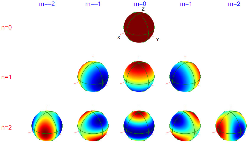Figure 1 Graphic of the spherical harmonic functions up to n=2 on the surface of the unit sphere. Notes: Here are illustrated the spherical harmonic patterns that gradient shim coils emulate with the Bz field they produce. (The labels X, Y, and Z identify the vectors of cartesian space). MRI terminology identifies n as the shim order, and degree m as one of the (2n +1) linearly independent degenerate functions associated with order n. (It should be noted that this differs from strict mathematical convention).

Broad classifications of shimming techniques: passive and active

Passive methods

Passive shimming methods employ materials that can support some level of magnetization (including diamagnetic and paramagnetic materials), and through strategic design and placement sculpt the magnetic field distribution toward a more uniform state via their passive response to the primary B₀ field. Due to the requirement that the necessary materials be physically positioned in the unit during the shimming process, clinical practice has generally excluded this method from being used on a patient-by-patient basis. Instead, its primary use has been the removal of hardware-related and environmental sources of field imperfection. A further complication regarding the use of passive shims is the temperature dependency of the induced magnetization.^18,19 Therefore, changes in temperature will cause the magnetic distribution created by the passive shims to change, with potentially detrimental effects on image quality and geometric accuracy. The implementation of passive shims must therefore proceed only with the awareness that their proper functioning depends on stable temperature conditions.

Active methods

The most prominent form of active shimming methods utilizes current-carrying loops that when activated can mitigate field imperfections within the bore. Superconducting magnets often utilize active superconducting shim coils that need only be set once during installation. These coils are used to full capacity to improve B₀ homogeneity so as to rely less on iron passive shim, whose response, as noted earlier, is temperature-sensitive and can lead to instability.¹⁸ However, perhaps the most noteworthy form of active shimming is that of multiple resistive coils that are designed to create magnetic fields that emulate the spatial variation of the spherical harmonic functions. The current in these coils can be varied at will on the MRI console, bestowing the ability to null out much of the unique distortion fields generated by the distribution of tissue magnetic susceptibility from each individual patient as they are scanned.

The use of current-carrying coils that comprise an orthogonal basis set for the correction of nonuniform fields for nuclear magnetic resonance was pioneered in the late 1950s.^12,20 These methods that began for shimming nuclear magnetic resonance spectrometers translated seamlessly into imaging systems. In 1984, Roméo and Hoult published a work that solidified a mathematical framework for both designing shim coils and field-mapping principles to identify the weighting for each harmonic term, and thus the current required for each coil.²¹ While shim coils have generally moved toward distributed current windings and optimization strategies, the design strategies proposed in this work remain relevant in current research.²²

The number of resistive shim coils to include in a system is an important consideration. Each shim coil will typically require its own separate power supply and control. Also, since the complexity and cost of an MRI system goes up with increases in patient-access dimensions (ie, bore diameter or interpole separation), the real estate occupied by shim coils is precious. It is largely for these reasons that so-called high-order shims (n=2 and above) are often not found in clinical magnets under 3 T, where susceptibility distortions are typically less severe. On 7 T commercial scanners, where susceptibility-induced fields are over four times the strength of the typical 1.5 T clinical magnet, complete third-order shims are typically present, bringing the number of resistive shim coils to 12 (not including B₀ and linear shims). While groups have shown some quantifiable benefits to the use of third-order shim terms,²³ there are some who feel that a second-order shim set with sufficient range of adjustment is sufficient for imaging and spectroscopy.²⁴

A secondary form of active shimming utilizes ferromagnetic materials with a high level of remanent magnetization and coercivity (ie, rare-earth magnets, such as NdFeB or SmCo). The high coercivity is fundamentally important to this procedure, as it allows the polarity and much of the remanent magnetization to remain constant regardless of its position or orientation within the primary magnet. In this way, its magnetization is no longer a passive response to B₀, but an independent field source. The ability for the polarity to be independent from the main field adds a great deal of flexibility to this current-free shimming procedure over passive means, and can be particularly useful for biplanar magnet designs.²⁵ Similar to the passive methods discussed earlier, the requirement that these magnets be physically positioned or repositioned every time the shim is to be corrected has limited the practicality of using this technique for susceptibility-related distortion on a subject-to-subject basis. Further, it should be noted that these magnets often exhibit significant temperature sensitivity (for example, ~1,200 ppm/°C for NdFeB),²⁶ so temperature stability is important for robustness.

Determination of harmonic coefficients

Regardless of what corrective means are used to produce the harmonic field distributions, before they are applied, one must find some method to identify the strength of the components that are present in the distortion field. The most basic of these methods is an iterative procedure, which may be undertaken manually or via an automated algorithm. As one can imagine, the manual option can be very time-consuming, and relies greatly on the experience and intuition of the operator. Here, the operator will view the free-induction decay and/or its frequency transform from an excitation of the VOI, the objective being a maximally prolonged free-induction decay with a nice exponential shape in the time domain, or a maximally narrow frequency-domain spectral peak with a symmetric shape. While finally attaining a beautiful shim on a sample is greatly satisfying, the time and the intricacy involved are distinct drawbacks, especially while a subject is waiting patiently in the unit. Another difficulty when shimming on a tissue volume in vivo is the fact that the VOI will frequently be displaced from the isocenter. In this situation, the manipulation of harmonics at higher orders will add lower-order terms.²⁷ (In essence, the spherical harmonics are no longer purely orthogonal on a shifted volume.) This can be remedied by adjusting the lower-order terms accordingly, but will add to the time and difficulty of the operation. Automated search algorithms can quickly take these calculable adjustments on lower-order terms into account. As a result, and because of their immunity to differing levels of operator expertise, they are clearly the better choice of clinical units. However, these automated methods can still be somewhat time-consuming, particularly when higher-order shims are involved.

The need for a rapid and automated method of determining the shim harmonic coefficients led Prammer et al in 1988 to develop a noniterative method to establish a shim solution in a single step through the use of spatial magnetic field mapping.²⁸ In this process, a three-dimensional assessment of the magnetic field within the sample or subject of interest was acquired with phase images at multiple planes. This field distribution was then mathematically nulled by calculating an optimal arrangement of shim-coil currents. Rather than assuming that each shim coil produced its intended spherical harmonic field pattern with perfect precision, the field distribution of each was experimentally mapped, generating a true basis set of the shim fields available. This approach was comparatively fast and much less likely to provide a local-minimum solution than the iterative methods mentioned earlier.

Despite the advantages of image-based approaches to the shim solution, the time required to acquire accurate and well-resolved field maps can still be undesirable. Consequently, in 1992 Gruetter and Boesch identified a set of precisely six frequency profiles that could be used to calculate the required coefficients for all first- and second-order shim terms.¹⁶ This led to the development of the FastMap algorithm,²⁹ which with its subsequent variants, such as Fast(er)Map³⁰ and Fast(est)Map,³¹ has been used heavily in the clinic ever since. While these are efficient methods of shimming over a specific volume, situations arise where one may need to consider different volumes simultaneously, sometimes with differing levels of restriction on field uniformity. For example, one may wish to establish a shim over a particular organ with a tight B₀ range, while maintaining a coarser uniformity over the entire abdominal slice to prevent frequency-based fat-suppression techniques from failing. By obtaining spatial field maps (typically by observing pixel phase drift over a multiple gradient-echo measurement), one can apply these types of constraints to determine the optimal harmonic coefficients for the situation at hand. Using this type of method, one also has the ability to identify arbitrary, irregular regions on which to optimize the shim. A rapid image-based procedure was introduced in 1995 by Reese et al,³² and has been developed by other groups in subsequent years.³³

Passive and active shimming strategies to combat local distortions with high spatial orders

Traditional passive and active shimming techniques have been used to great effect in preparing a uniform B₀ field in the absence of a patient, as well as responding to the distorting fields created by the patient’s presence in the form of active shim coils emulating spherical harmonic functions. However, as indicated earlier, the complex geometries of tissue structures and air can create distorting fields for which second- and even third-order harmonics are insufficient, particularly as high field strengths become more commonplace. To combat this issue without resorting to the costly and technically taxing extreme of adding higher and higher orders of shim sets, groups have come up with a number of novel alternate methods, some of which may well appear in the clinic in years to come.

Passive strategies

Intraoral pyrolytic graphite insert

Maintaining B₀ uniformity over the brain is a challenging problem, based on the complex geometry of air, soft tissue, and bone, and the common need to perform imaging sequences that are particularly sensitive to B₀ fluctuations (ie, echo planar imaging (EPI) commonly used for functional MRI [fMRI] studies). In 2002, Wilson et al published a novel method to combat the distortion often seen in the inferior frontal cortex.³⁴ Here, an insert composed of pyrolytic carbon (example shown in Figure 2) was held in the mouth of volunteers during a 3 T scan to reduce the intensity of the field induced primarily by the ethmoid and sphenoid sinuses. Pyrolytic carbon, being highly diamagnetic (with a negative susceptibility as strong as –450 ppm at certain orientations),³⁵ when placed inferior to the sinus served to reduce its effect on the field uniformity of the inferior frontal cortex. This was further demonstrated by Cusack et al in 2004, who investigated its efficacy for fMRI use.³⁶

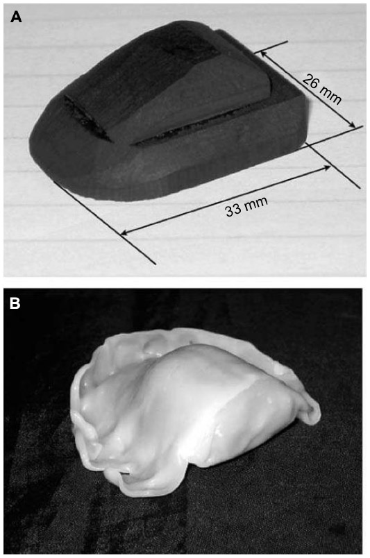Figure 2 Passive intra-oral shim made of pyrolytic graphite. Notes: (A), pyrolytic graphite intraoral shim; (B), plastic mold that contained it. Reprinted from NeuroImage, 24(1), Cusack R, Russel B, Cox SM, De Panfilis C, Schwarzbauer C, Ansorge R, An evaluation of the use of passive shimming to improve frontal sensitivity in fMRI, 82–91, Copyright © 2005, with permission from Elsevier.36

Arrangements of permalloy to create a passive harmonic basis set

On a local spatial scale, the field distortions induced by susceptibility differences can often be of a greater intensity than the integrated active higher-order shim sets can achieve, especially at higher fields, as noted by Juchem et al in 2006.³⁷ In this work, a method was proposed to create a second-order basis set via passive means that could greatly augment the capacity of the system to correct for local distortions of this order. This basis set was constructed on a cylindrical form with strips of an Ni–Fe alloy (permalloy) on a subject-specific basis (see Figure 3). The passive basis set was used to achieve a rough field correction, after which an onboard active shim set was used to fine-tune the field.

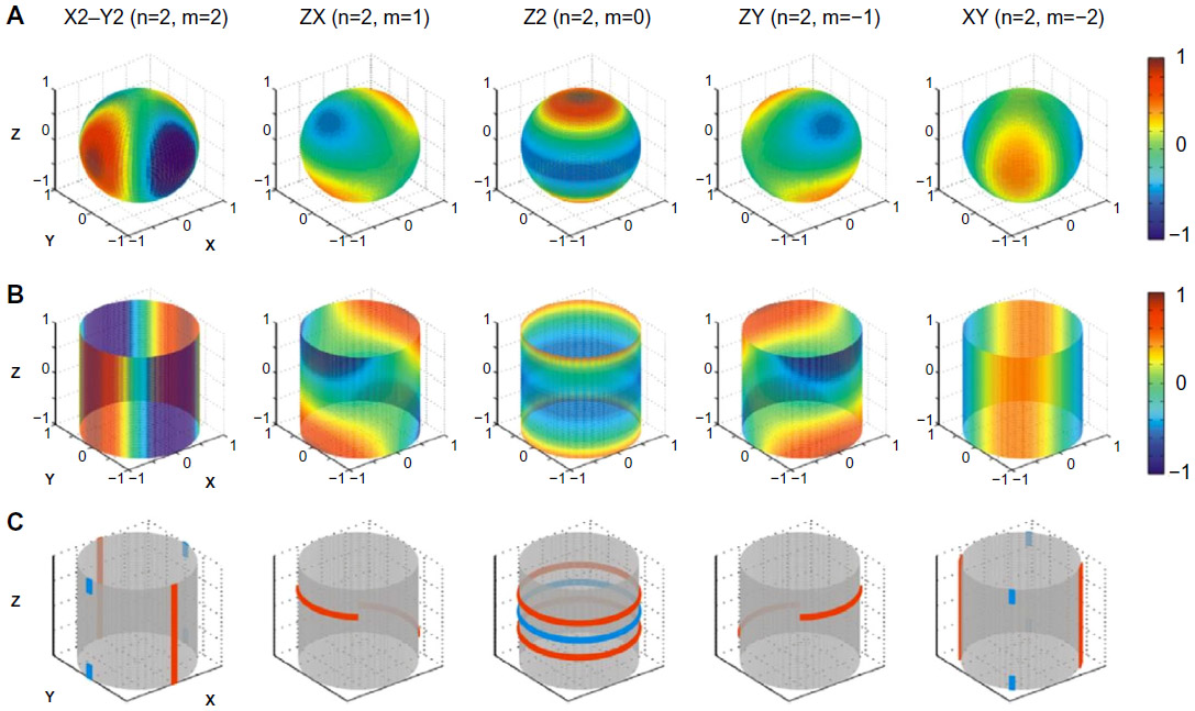Figure 3 Passive permalloy shim solutions for a second-order shim set. Notes: 3-D visualization of the second-order spherical harmonic functions X2–Y2, ZX, Z2, ZY, XY (n=2, m=−2, −1, 0, 1, and 2) for a unit sphere (A) and for a unit cylinder (B). In figure part C the red lines represent the theoretically optimized permalloy-shim solutions intended to reproduce the fields seen in the upper two rows, with two pieces of permalloy per shim. Blue lines represent alternate solutions, which allow for minimization of materials at a cost of field accuracy. Reprinted from the Journal of Magnetic Resonance, 183(2), Juchem C, Muller-Bierl B, Schick F, Logothetis NK, Pfeuffer J, Combined passive and active shimming for in vivo MR spectroscopy at high magnetic fields, 278–289, Copyright © 2006, with permission from Elsevier.37

Subject-specific shimming systems using nonharmonic distributions of materials with magnetic properties

There have been a number of ideas developed over the last decade or so that accomplish a shim over a target region by strategically distributing material with magnetic properties at precise positions about the subject. Rather than using the magnetic materials to construct various specific spherical harmonic terms, these methods used numerical optimizations to identify the best distribution to combat the distortion in the target region. This has the potential advantage of including a wider array of spatial orders in its solution. One such solution was presented in 2006 by Koch et al, in which a structure was described that could hold an array of paramagnetic and diamagnetic materials (zirconium and bismuth in this report) positioned on a cylindrical form for mouse imaging.³⁸ Here, rectangular pieces of these materials were placed in a grid-like fashion around the cylinder (see Figure 4). The number of pieces to be placed at each grid location, whether a single material or a combination of both, was determined by fitting the target field to an array of unit-response distributions appropriate for each location on the grid. By combining paramagnetic and diamagnetic materials, the authors were able to achieve a range of effective susceptibility at each grid point, allowing for more exact field solutions.

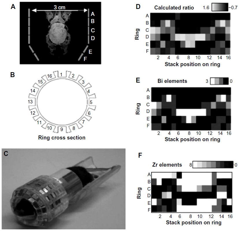Figure 4 Passive shim assembly for a mouse head. Notes: (A) Coronal cross section of the mouse-shim system, with rings labeled by letters A to F. (B) Ring cross section, showing ring geometry and ring positions labeled by number. (C) Photograph of constructed shim assembly. (D–F) Optimized ratios and corresponding sheet numbers of bismuth (Bi) to zirconium (Zr). Reprinted from the Journal of Magnetic Resonance, 182(1), Koch KM, Brown PB, Rothman DL, de Graaf RA, Sample-specific diamagnetic and paramagnetic passive shimming, 66–74, Copyright © 2006, with permission from Elsevier.38

In 2011, Yang et al published a strategy of this type for the shimming of human brain in vivo.³⁹ It did not utilize a grid, as in the strategy just mentioned, but four small cylindrically-shaped pieces of paramagnetic niobium metal fixed onto a frame. The frame, secured to a head coil, could position the pieces at precise and adjustable locations around the subject (see Figure 5). An analytic expression was used to describe the induced magnetic field distribution around each cylinder, which could then be used to determine optimal positions for each of the niobium pieces. This optimization was achieved by using a numerical routine that varied the positions of the cylinders until the induced field from each best compensated for the B₀ inhomogeneity measured in the target region.

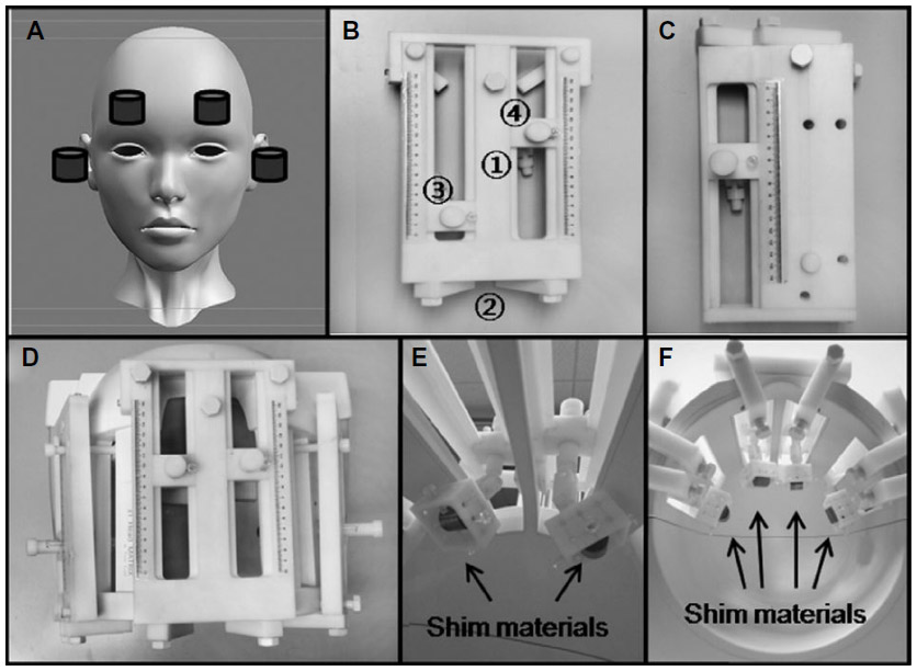Figure 5 A passive shim assembly for the human head using niobium cylinders. Notes: (A) Typical optimized locations of niobium cylinders relative to the head. (B and C) Frontal and temporal lobe shim-structure assemblies. The circled numbers identify different components on the frontal lobe assembly. (1) identifies the primary assembly. (2) identifies the mounting structure, and (3) and (4) identify the adjustable controllers, by which the niobium cylinders can be repositioned. (D–F) Assemblies mounted on head coil. Reprinted from Magnetic Resonance Imaging, 29(3), Yang S, Kim H, Ghim MO, Lee BU, Kim DH, Local in vivo shimming using adaptive passive shim positioning, 401–407, Copyright © 2011, with permission from Elsevier.39

Finally, an older but unique solution was presented in 2001 by Jesmanowicz et al, in which the thickness of a ferromagnetic layer of photocopier toner was optimized, printed, and wrapped around a cylindrical form.⁴⁰ This optimization included the use of zero- to second-order shim terms in order to identify a minimal layer of toner that would produce a satisfactory solution.

Susceptibility matching

While not a high-tech solution, the use of a material to match tissue susceptibility on an external body surface can be a very effective and straightforward solution to minimizing the detrimental effects of an air–tissue interface close to a region of interest (ROI). This method works primarily by displacing the air interface to a more distant location, but also by replacing potentially complex geometries (likely to produce B₀ field distortions with high spatial orders) with hopefully simpler and more slowly varying ones. Of particular interest are those materials that both achieve a reasonable tissue-susceptibility match and do not contribute a measurable MR signal. Perfluorocarbon liquids, such as Fluorinert (FC-77 by 3M), are one such material, and have become frequently seen in the MR literature.⁴¹ There are other successful materials in this regard: Moriya et al reported in 2010 that bags of dried rice performed better for improving fat suppression near air interfaces than did the perfluorocarbon liquid.⁴²

Active strategies

Local control of B₀ distortion through strategically placed electrical coil loops

To combat field distortion in the inferior frontal lobe resulting from air pockets in the sinuses and nasal cavity, Hsu and Glover reported in 2005 on the use of a set of three small coil loops that could operate intraorally.⁴³ This part of the brain is a frequent site of B₀ field distortion, which is particularly problematic for fMRI studies. While similar in intent to the passive pyrolytic carbon device discussed earlier, the fields created by these coils were easily adjustable on a subject-specific basis. After patient setup, a conventional shim was first implemented over the brain based on three linear gradient fields. Subsequently, the response of each oral shim coil was independently calibrated by mapping out the magnetic field distribution created by each in response to a known current input. A least squares fitting procedure was then used to determine optimal drive currents for each intraoral coil, as well as optimal adjustments to the linear shim fields that would be required to best null out the field variation measured over a particular ROI.

To address the same problem, Juchem et al in 2010 proposed a set of six coils, all positioned externally to the patient, which could reduce this susceptibility-related distortion.⁴⁴ The position and dimension of these six coil loops was determined in a manner so as to be suitable for heads of all sizes, based on a set of 15 volunteers. The current through each of these coils could then be adjusted on a subject-specific basis. The optimized sizes and positioning of the coils were determined both to counteract the general field-distortion pattern in the prefrontal cortex that was common to most people, as well as to avoid introducing distortions to other parts of the brain.

Multicoil array of electrical coil loops

Starting in 2009, Juchem et al published a number of articles outlining a novel method of generating rather arbitrary magnetic field distributions, including spherical harmonic functions up to fourth order, with a single grid of circular coils arranged around a cylindrical form.^45,46 The method was demonstrated in mice with a 48-loop array (Figure 6), in which the multicoil approach was shown to outperform a second-order spherical harmonic shim set.⁴⁷ The multicoil approach was likewise demonstrated in a human brain at 7 T (Figure 7).⁴⁸ The latest publication used modeling techniques to evaluate efficiency in creating shims of various spatial orders versus shims with equivalent orders created by traditional spherical harmonic coil sets.⁴⁹ This publication reported a roughly equivalent efficiency for linear harmonic terms, and an advantage of roughly 1.5 and 3.5 for second- and third-order harmonic terms, respectively.

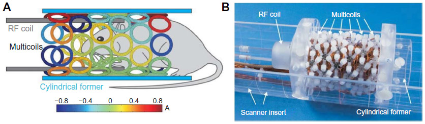Figure 6 Multicoil active shim assembly for mouse imaging/spectroscropy. Notes: (A) Schematic of the 48-loop multicoil shim setup. Colors on individual coils indicate an example of coil currents required for the shimming of a mouse brain. (B) Experimental realization of the design. Copyright © 2011 Wiley-Liss, Inc., reprinted from Multicoil shimming of the mouse brain, Juchem C, Brown PB, Nixon TW, McIntyre S, Rothman DL, de Graaf RA, Magnetic Resonance in Medicine, 66(3),893–900.47 Abbreviation: RF, radio-frequency.

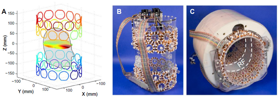Figure 7 Multicoil shim assembly for the human head. Notes: (A) Schematic of the 48-loop multicoil shim for a head coil at 7 T. (B and C) Experimental realization of the design. Reprinted from Journal of Magnetic Resonance, 212(2), Juchem C, Nixon TW, McIntyre S, Boer VO, Rothman DL, de Graaf RA, Dynamic multi-coil shimming of the human brain at 7 T, 280–288, Copyright © 2011, with permission from Elsevier.48 Abbreviation: RF, radio frequency.

Discussion

Addressing local distortions with high spatial orders is the modern thrust of development in MRI field shimming. With the higher field strengths that are becoming more common both for animal imaging as well as human imaging in vivo, the tried-and-true spherical harmonic basis sets that have served MRI well for decades are showing more and more limitations. These limitations are in particular related to the distortions arising from susceptibility distributions, whose detrimental effects on field homogeneity increase with B₀. Both passive and active means have been shown to address these issues in a variety of situations. However, passive approaches will be less likely to be incorporated in a routine fashion in the clinic, due to the practical matter of physically placing and/or optimizing the passive shim components to reflect the subject-specific field distribution. There may well be specific situations where the passive approach is simple and effective enough to become standard. More than likely, if and when passive methods are used, it will be because the active shim methods available do not have the strength or spatial resolution to correct field nonuniformities with high-order terms, in which case a combination of passive and active methods will be needed.

The multicoil arrays have the promise to one day potentially replace the standard shim sets that are common today with a compact unit that is capable of creating high-order spatial distributions of field. Additionally, the extra degrees of freedom that they offer would permit one ROI to be well treated with high-order correction without compromising the homogeneity of the surrounding areas, a problem that one faces today when using spherical harmonic terms alone. However, before this transition could happen, there would have to be many thorough evaluations of effectiveness and efficiency over a wide range of applications, including shim sets designed for whole-body units.

Disclosure

The author reports no conflicts of interest in this work.

---

References

1.	Tofts PS. Modeling tracer kinetics in dynamic Gd-DTPA MR imaging. J Magn Reson Imaging. 1997;7(1):91–101.
2.	Ogawa S, Lee TM, Kay AR, Tank DW. Brain magnetic resonance imaging with contrast dependent on blood oxygenation. Proc Natl Acad Sci U S A. 1990;87(24):9868–9872.
3.	Rieke V, Butts-Pauly K. MR thermometry. J Magn Reson Imaging. 2008;27(2):376–390.
4.	Sun PZ, Sorensen AG. Imaging pH using the chemical exchange saturation transfer (CEST) MRI: correction of concomitant RF irradiation effects to quantify CEST MRI for chemical exchange rate and pH. Magn Reson Med. 2008;60(2):390–397.
5.	Manduca A, Oliphant TE, Dresner MA, et al. Magnetic resonance elastography: non-invasive mapping of tissue elasticity. Med Image Anal. 2001;5(4):237–254.
6.	Larson PS, Starr PA, Bates G, Tansey L, Richardson RM, Martin AJ. An optimized system for interventional magnetic resonance imaging-guided stereotactic surgery: preliminary evaluation of targeting accuracy. Neurosurgery. 2012;70(1 Suppl Operative):95–103.
7.	Wachowicz K, Tadic T, Fallone BG. Geometric distortion and shimming considerations in a rotating MR-linac design due to the influence of low-level external magnetic fields. Med Phys. 2012;39(5):2659–2668.
8.	Martinez-Möller A, Eiber M, Nekolla SG, et al. Workflow and scan protocol considerations for integrated whole-body PET/MRI in oncology. J Nucl Med. 2012;53(9):1415–1426.
9.	Poole M, Bowtell R. Novel gradient coils designed using a boundary element method. Concepts Magn Reson Part B Magn Reson Eng. 2007;31(3):162–175.
10.	Janke A, Zhao H, Cowin GJ, Galloway GJ, Doddrell DM. Use of spherical harmonic deconvolution methods to compensate for nonlinear gradient effects on MRI images. Magn Reson Med. 2004;52(1):115–122.
11.	Kristensena BH, Laursena FJ, Løgager V, Geertsen PF, Krarup- Hansen A. Dosimetric and geometric evaluation of an open low-field magnetic resonance simulator for radiotherapy treatment planning of brain tumours. Radiother Oncol. 2008;87(1):100–109.
12.	Golay MJ. Field homogenizing coils for nuclear spin resonance instrumentation. Rev Sci Instrum. 1958;29(4):313–315.
13.	Koch KM, Rothman DL, de Graaf RA. Optimization of static magnetic field homogeneity in the human and animal brain in vivo. Prog Nucl Magn Reson Spectrosc. 2009;54(2):69–96.
14.	Schenck JF. The role of magnetic susceptibility in magnetic resonance imaging: MRI magnetic compatibility of the first and second kinds. Med Phys. 1996;23(6):815–850.
15.	Murashima M, Ueno T, Sugimoto N. Effective digitized spatial size of unit dipole field in quantitative susceptibility mapping. Poster presented at: 35th Annual International Conference of the IEEE Engineering in Medicine and Biology Society; July 3–7, 2013; Osaka, Japan.
16.	Gruetter R, Boesch C. Fast, noniterative shimming of spatially localized signals. In vivo analysis of the magnetic field along axes. J Magn Reson. 1992;96:323–334.
17.	de Graaf RA. In Vivo NMR Spectroscopy: Principles and Techniques. 2nd ed. Chichester, UK: John Wiley and Sons; 2007.
18.	Hillenbrand DF, Lo KM, Punchard WF, Reese TG, Starewicz PM. High-order MR shimming: a simulation study of the effectiveness of competing methods, using an established susceptibility model of the human head. Appl Magn Reson. 2005;29(1):39–64.
19.	Liu F, Zhu J, Xia L, Crozier S. A hybrid field-harmonics approach for passive shimming design in MRI. IEEE Trans Appl Supercond. 2011;21(2):60–67.
20.	Anderson WA. Electrical current shims for correcting magnetic fields. Rev Sci Instrum. 1961;32(3):241–250.
21.	Roméo F, Hoult DI. Magnet field profiling: analysis and correcting coil design. Magn Reson Med. 1984;1(1):44–65.
22.	Liu W, Tang X, Zu D. A novel target-field approach to design bi-planar shim coils for permanent-magnet MRI. Concepts Magn Reson Part B Magn Reson Eng. 2010;37(1):29–38.
23.	Pan JW, Lo KM, Hetherington HP. Role of very high order and degree B0 shimming for spectroscopic imaging of the human brain at 7 tesla. Magn Reson Med. 2012;68(4):1007–1017.
24.	Schmitt F, Potthast A, Stoeckel B, Triantafyllou C, Wiggins CJ. Aspects of clinical imaging at 7 T. In: Robitaille PM, Berliner L, editors. Ultra High Field Magnetic Resonance Imaging. New York: Springer; 2006.
25.	Hong L, Zu D. Shimming permanent magnet of MRI scanner. Prog Electromagn Res Symp. 2007;3(6):859–864.
26.	Haishi T, Uematsu T, Yoshimasa M, Katsumi K. Development of a 1.0 T MR microscope using a Nd-Fe-B permanent magnet. Magn Reson Imaging. 2001;19(6):875–880.
27.	Hoult DI. “Shimming” on spatially localized signals. J Magn Reson. 1987;73(1):174–177.
28.	Prammer MG, Haselgrove JC, Shinnar M, Leigh JS. A new approach to automatic shimming. J Magn Reson. 1988;77(1):40–52.
29.	Gruetter R. Automatic, localized in vivo adjustment of all first- and second-order shim coils. Magn Reson Med. 1993;29(6):804–811.
30.	Shen J, Rycyna RE, Rothman DL. Improvements on an in vivo automatic shimming method (FASTERMAP). Magn Reson Med. 1997;38(5):834–839.
31.	Gruetter R, Tkác I. Field mapping without reference scan using asymmetric echo-planar techniques. Magn Reson Med. 2000;43(2):319–323.
32.	Reese TG, Davis TL, Weisskoff RM. Automated shimming at 1.5 T using echo-planar image frequency maps. J Magn Reson Imaging. 1995;5(6):739–745.
33.	Wilson JL, Jenkinson M, de Araujo I, Kringelbach ML, Rolls ET, Jezzard P. Fast, fully automated global and local magnetic field optimization for fMRI of the human brain. Neuroimage. 2002;17(2):967–976.
34.	Wilson JL, Jenkinson M, Jezzard P. Optimization of static field homogeneity in human brain using diamagnetic passive shims. Magn Reson Med. 2002;48(5):906–914.
35.	Simon MD, Heflinger LO, Geim AK. Diamagnetically stabilized magnet levitation. Am J Phys. 2001;69(6):702–713.
36.	Cusack R, Russel B, Cox SM, De Panfilis C, Schwarzbauer C, Ansorge R. An evaluation of the use of passive shimming to improve frontal sensitivity in fMRI. Neuro Image. 2005;24(1):82–91.
37.	Juchem C, Muller-Bierl B, Schick F, Logothetis NK, Pfeuffer J. Combined passive and active shimming for in vivo MR spectroscopy at high magnetic fields. J Magn Reson. 2006;183(2):278–289.
38.	Koch KM, Brown PB, Rothman DL, de Graaf RA. Sample-specific diamagnetic and paramagnetic passive shimming. J Magn Reson. 2006;182(1):66–74.
39.	Yang S, Kim H, Ghim MO, Lee BU, Kim DH. Local in vivo shimming using adaptive passive shim positioning. Magn Reson Imaging. 2011; 29(3):401–407.
40.	Jesmanowicz A, Roopchansingh V, Cox RW, Starewicz P, Punchard WF, Hyde JS. Local ferroshims using office copier toner. Poster presented at: 9th Annual Scientific Meeting of the International Society for Magnetic Resonance Medicine; April 21–27, 2001; Glasgow, UK.
41.	Neufeld A, Assaf Y, Graif M, Hendler T, Navon G. Susceptibility-matched envelope for the correction of EPI artifacts. Magn Reson Imaging. 2005;23(9):947–951.
42.	Moriya S, Miki Y, Yokobayashi T, et al. Rice and perfluorocarbon liquid pads: comparison of fat suppression effects. Acta Radiol. 2010;51(5):534–538.
43.	Hsu JJ, Glover GH. Mitigation of susceptibility-induced signal loss in neuroimaging using localized shim coils. Magn Reson Med. 2005;53(2):243–248.
44.	Juchem C, Nixon TW, McIntyre S, Rothman DL, de Graaf RA. Magnetic field homogenization of the human prefrontal cortex with a set of localized electrical coils. Magn Reson Med. 2010;63(1):171–180.
45.	Juchem C, Rothman DL, de Graaf RA. First- to fourth-order spherical harmonics shimming with a grid of circular electrical coils. Poster presented at: Proceedings of the 17th Annual Scientific Meeting of the International Society for Magnetic Resonance Medicine; April 18–24, 2009; Honolulu, HI.
46.	Juchem C, Nixon TW, McIntyre S, Rothman DL, de Graaf RA. Magnetic field modeling with a set of individual localized coils. J Magn Reson. 2010;204(2):281–289.
47.	Juchem C, Brown PB, Nixon TW, McIntyre S, Rothman DL, de Graaf RA. Multicoil shimming of the mouse brain. Magn Reson Med. 2011;66(3):893–900.
48.	Juchem C, Nixon TW, McIntyre S, Boer VO, Rothman DL, de Graaf RA. Dynamic multi-coil shimming of the human brain at 7 T. J Magn Reson. 2011;212(2):280–288.
49.	Juchem C, Green D, de Graaf RA. Multi-coil magnetic field modeling. J Magn Reson. 2013;236:95–104.