Effect of health development assistance on health status in sub-Saharan Africa

Introduction

For decades, health has been recognized to be a salient input for economic development as a healthier population can raise the productivity of the labor force while reducing poverty.¹ At the same time, health is increasingly viewed as a basic human right, the fulfillment of which is an obligation for both developed and developing countries.²

According to World Bank data,³ in sub-Saharan Africa (SSA), the infant mortality rate (IMR) was 137 during the 1960s. During the same period, in Latin America and the Caribbean region, this health indicator was 91, whereas it was 31 in the high-income Organization for Economic Cooperation and Development (OECD) countries. Even during the implementation period of the millennium development goals (MDGs), in the years between 2001 and 2010, the SSA region was only able to reduce the IMR to 72, but the OECD was successful in reducing this indicator to four. This figure indicates that during this decade, saving the lives of approximately 68 infants was not beyond human capacity, even if it was beyond SSA’s capacity. But multitudes of factors related to people’s living standards contributed to such a disturbing condition of life.³

Considering this discrepancy, mobilizing more resources to improve health in developing countries has been a global concern for decades, as evidenced by the unprecedented rise in development assistance for health (DAH) (DAH is generally defined as external resources, financial or in-kind, that are channeled into a country from external sources to support health-related activities. It generally includes funding for health sector activities, as well as population programs, but generally does not include activities outside the health sector that may affect health [eg, water and sanitation programs]), hereafter termed as health development aid (HDA). Also seen is the emergence of several new global health-financing institutions during the past 2 decades to address the complex problem of health status in developing countries.⁴

Furthermore, this has been well reflected in the recently accomplished MDGs, wherein three out of the eight goals were directly related to health: reduction of child mortality; maternal health improvement; and combating HIV/AIDS, malaria, and, other diseases.

Thus, health aid in the form of HDA remains one major source financing the health sector in developing countries in general and in SSA in particular because of the fact that the region has been a major recipient of health aid for decades. Even if all recipient regions of the world had increased HDA funding from 1990, the relative share of SSA increased from 9.7% in 1990 to 13.8% in 2001, and then to 22.7% in 2007.⁴ Similarly, health aid disbursement in the region has increased from 1 billion USD in 2000 to 4 billion USD in 2009.^5,6 While there have been undeniable improvements in health status of the region during the past 2 decades, whether the improvements can be attributed to the HDA is inconclusive.

Despite the ample empirical research results we have in the literature on the effect of foreign aid on economic growth, there is scarcity of evidence that deals with the effects of health-targeted aid in the form of HDA. Within the available literature itself, there is also a lack of consensus concerning the effect of health aid in developing countries. On one side, researchers argue that health-specific aid leads to improved health outcomes in developing countries by relaxing resource constraints and directly improving health service delivery.^7–9 According to one systematic review,¹⁰ interventions in terms of HDA also appear to be associated with improvements, although small, in maternal health outcome. On the other side, scholars argue that there is no such reliable empirical evidence supporting the claimed positive effect of health aid on health outcome. They argue that funds going to the health sector basically have no impact on the level of health status indicators across countries.^10–14

Although SSA is the biggest recipient of HDA, evidence on the relationship between HDA and health status outcome in the region is very limited. The few available studies make use of a full sample of developing countries, though controlled for the region using regional dummies. Moreover, most of the previous studies make use of HDA data on commitments,^7,8,12 which may not necessarily be the actual amount of aid that the recipient country utilized. To get a more assertive result concerning the effect under consideration in the region, we feel the region needs to be investigated separately, using actual health expenditure sourced from external assistance instead of aid commitment data.

Methods

Panel data analytic method, which is an increasingly popular form of cross-sectional time series data analysis in econometrics, was used in this study. The method combines cross-sectional and time series data together to get more reliable parameter estimates than what either the cross-section or the time series approach alone may give.¹⁵ Therefore, this study used cross-sectional and annual time series data for 43 SSA regions (Angola, Benin, Botswana, Burkina Faso, Burundi, Cameroon, Central African Republic, Chad, Comoros, Congo, Democratic Republic of the Congo, Cote d’Ivoire, Equatorial Guinea, Eritrea, Ethiopia, Gabon, Gambia, Ghana, Guinea, Guinea-Bissau, Kenya, Lesotho, Liberia, Madagascar, Malawi, Mali, Mauritania, Mauritius, Mozambique, Namibia, Niger, Nigeria, Rwanda, Senegal, Seychelles, Sierra Leone, South Africa, Sudan, Swaziland, Tanzania, Togo, Uganda, and Zambia). In forming the panel, for both the dependent and explanatory variables, the time series data of each country were averaged over 5 years and a total of four time data points were formed for each country.

The model

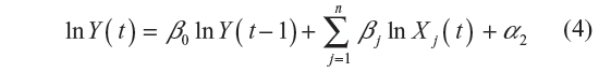
Empirical investigation of the effect of HDA on health outcome requires specifying the health outcome estimating equation. On the basis of the bulk of the previous literature,^8,12–15 three such equations were derived by transforming implicit functions that contain explanatory variables as determinants in their explicit mathematical forms by making some plausible assumptions. The first model, hereafter termed Model I, assumes the stability of elasticities of health status with respect to the identified explanatory variables without controlling for the previously existing level of health status. In other words, this model assumes that a given percentage change causes some given percentage change on health status, irrespective of previously existing level of health status.

Mathematically, if the health outcome at time t is denoted by Y(t) and its determinants at time t by X₁(t), X₂(t), …, X_n(t), where the X_i(t) terms include variables such as HDA, household income, education, sanitation facilities, human health–related ecosystem, and quality of governance, then, from an implicit function:

by taking the total derivative of both sides of the equation and dividing both sides by Y(t), one gets the following:

where is Y(t)’s elasticity with respect to X_j(t), f_j is the marginal effect of X_j(t) on Y(t), and j = 1,2, …, n.

As pointed out earlier, using the assumption of constant elasticities, one can integrate both sides of the equation, and get the following:

where α₁ is some constant term.

Thus, Model I, which assumes that ε_j is constant, is equivalent to stating the required health status–estimating equation in a static log-linear form.

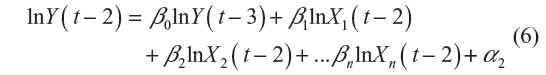
The second model, hereafter termed Model II, assumes the stability of the elasticities of health status with respect to its determinants “after” controlling for the previous level of health status. In other terms, this model assumes the existence of some constant percentage change in health status as a result of a given percentage change in the explanatory variables only for specific previously existing levels of health status.

Intuitively, one understands the possibility that the coefficients in the health status estimating Equation 3 could be related to the level of health status before a change in the explanatory variables takes place. That is, keeping other things unchanged, a 1% change in HDA when the recipient economy exists at a lower level of health status could have much better effects than when similar change in the assistance is applied to another economy with a higher level of health status. This is because in low-income countries, most often, health is endangered due to lack of some very basic necessities of life, which may be fulfilled with low expenses. This phenomenon demands us to control for previous level of health status if we need to find a more refined parametric effect of health aid on health status. Moreover, in real cases, besides the indicated level effect, the explanatory variables could have lagged effects in addition to their present effects. For instance, HDA that is channeled at a present time, say, for training of health personnel or for buying medical equipment, vehicles, or buildings could have both current and lagged effects. The same is true for other explanatory variables.

These conditions require us to take the lagged effects of our outcome variable and the explanatory variables into account to give an unbiased estimation of the coefficient. Including lagged outcome variables in the model can also control for many omitted-variable biases to a large extent. Notice that under some mathematical restrictions, the inclusion of lagged health status level in the equation is equivalent to incorporating all past lagged effects of the explanatory variables.

To observe the fact that Equation 4 captures the lagged effects of explanatory variables on the dependent variable as well, one may lag the dependent variable by one period and substitute the expression on the right hand side in Equation 4. Repeating the same action by lagging the dependent variable by two, three periods and so on and substituting the results in the original equation, the ultimate equation will be an expression of the dependent variable in terms of all the present and past values of the explanatory variables. That is by lagging the Equation 4 by one period, we get the following:

Repeating the same action on Equation 5, we get the following:

and so on, and then substituting Equation 6 in Equation 5 and substituting Equation 5 in Equation 4, one gets a general equation as follows:

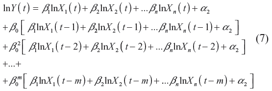
where m is the maximum possible lag in years. Equation 7 expresses the present level of health status in terms of all the possible lags of explanatory variables. Moreover, the equation implies that the lagged effects of the explanatory variables decay with time as far as 0 < β₀ < 1.

Accordingly, the implicit function of health status that includes the lagged level of health status among the explanatory variables is expressed as

where n is the number of explanatory variables.

As in the case of Model I, taking the derivative of both sides of the equation and dividing both sides by Y(t), we get

where β₀ is Y(t)’s elasticity with respect to Y(t −1).

Under the indicated assumption, one can integrate both sides of the equation and get Equation 4, where α₂ is some constant term.

That is, Model II, which assumes the stability of β after controlling for previous level of health status is equivalent to stating the required health status–estimating equation in a dynamic log-linear form. Notice that even if Model I and Model II are very common types in empirical research, both presume the possibility of sustained improvements in health status. That is, if one or more of the explanatory variables exhibit sustained growth, say, such as the case of per capita income growth, then these models predict the possibility of sustained growth in health status.

The third model, hereafter termed Model III, assumes stability of the product of the elasticities and health status instead of stability of the elasticities. It also assumes stability of marginal effect of previous level of health status on the present level of health status. The implicit function for this model is identical with that of Model II and is expressed as

where n is the number of explanatory variables. Here again, by taking the derivative of both sides of the equation, we get

where f_j is the marginal effect of X_j(t) on Y(t), f₀ is the marginal effect of Y(t −1) on Y(t), and j = 1,2, …, n, which can be rewritten as

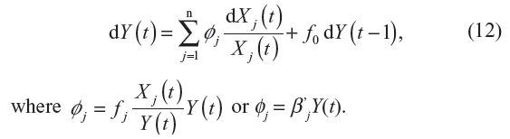
Under the assumptions indicated earlier, ie, constant φ_j values, one can integrate both sides of the equation and get

where δ = f₀ and α₃ is some constant term. Notice that under the assumption of constant φ_j values, as the health status is raised, the elasticity will fall, and vice versa. In this process, when the health status reaches some given maximum, the elasticities will take their minimum value. Thus, Model III is equivalent to stating the required health status–estimating equation in dynamic semilog-linear form.

Notice that Model III, while retaining most of the useful properties of Model I and Model II, avoids the implausible prediction of Model II in the cases of extreme level of health status.

Even if the choice among these models is made based on the extent to which they fit to the data, and will be done accordingly here, the advantage of Model III is that the coefficient estimates can inform the unit change in health status level as a result of a 1% change in the explanatory variables.

Model estimation

Estimation using Models I, II, and III requires specification of a function relating health outcome to a vector of explanatory variables such as HDA, household income, education, sanitation facilities, ecosystem indicators, quality of governance, and other health-related variables. However, here, due to data limitation, the econometric specification that related health status to a vector of explanatory variables under the assumption of Model I is given as follows:

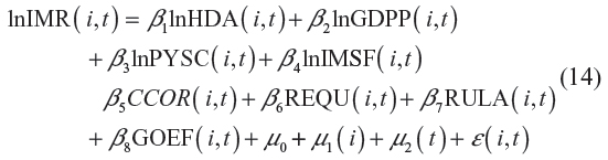
where ln IMR (i,t) is the log-infant mortality rate, ln HDA (i,t) is the log-health development assistance, ln GDPP (i,t) is the log-gross domestic product (GDP) per capita (GDPP), ln PYSC (i,t) is the log-primary years of schooling, ln IMSF is log-improved sanitation facilities, CCOR(i,t) is control of corruption, REQU (i,t) is the regulatory quality, RULA (i,t) is rule of law, and GOEF (i,t) is Government effectiveness, in country i at time t for i=1,2, …, 43 (number of countries), t=1,2,3,4 (number of time units); ε(i,t) is an error term with the property E[e(i,t)]=0 and var[e(i,t)]=(σ_e)²; μ₀ is a constant term; and μ₁(i) and μ₂(t) are country- and time-specific effects, respectively. In this specification, β_j terms fulfill the assumptions of Model I. To estimate Equation 14, two estimators were compared and the one that corresponded to the data better was selected based on some statistical tests. These estimators were the fixed-effect estimator, which assumes that there are constant country-specific effects, and the random-effects estimator, which assumes that there are random country-specific effects. To choose between the fixed-effect and random-effect estimators, ie, which one fits the data better, the Hausman specification test was conducted.

As indicated herein, Equation 4 suggests that if a given dependent variable is specified in an autoregressive form, then that may mean that the dependent variable is determined not only by the current effects of the explanatory variables but also by their lagged values. In our case here, estimation of the IMR-estimating equation specified in an autoregressive form such as Equation 4 helps to capture the lagged effects of the explanatory variables rather than assuming them away. Accordingly, Equation 14 is respecified in autoregressive form as follows:

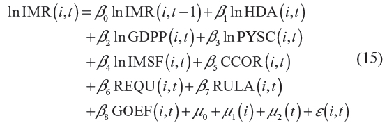
where ln IMR(i, t–1) is the log of IMR lagged by one period for country i, and other variables and parameters are as defined in Equation 14.

Furthermore, under the assumptions of Model III, the econometric specification that relates the dependent variable (IMR) to the vector of the explanatory variables is given as

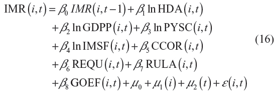
where IMR (t –1) is the lagged value of the dependent variable – IMR – and the other variables are as defined in Equation 14. In this specification, the β_j terms fulfill the assumptions of Model III.

The suitable estimator for dynamic panel models such as Equation 15 or Equation 16 would be either the first-difference generalized method of moments (GMM), developed by Arellano and Bond,¹⁶ or the system GMM, developed by Blundell and Bond,¹⁷ depending on the nature of the error terms. In general, the log of IMR is expected to have an autoregressive parameter far lesser than unity because the series tends to move to some stable level, say, close to zero, instead of persistently falling or rising at some constant rate. But Alonso-Borrego and Arellano¹⁸ indicated that system GMM is more appropriate in cases where the autoregressive parameter is closer to unity. Hence, here, first-difference GMM is preferred to system GMM. Using the first-difference GMM, the estimator Equation 15 and Equation 16 are estimated. The preferred GMM estimator also enables to surmount the endogeneity problem mainly caused by omitted variables or measurement errors in the estimation equation.

Data and variables

Health status has no unanimously accepted unit of measure. Instead, usually at the aggregate level of empirical research, mortality rate and life expectancy at birth are considered proxies or indicators of the status. For this study, to examine the effect of HDA on health status, IMR was taken as a proxy for health status because it is more appropriate than life expectancy in the case of low-income countries.⁸ Obviously, the attempt at estimating the effect of health aid demands controlling for other effects that arise from other socioeconomic variables. For this purpose, in addition to the main variable of interest – HDA – per capita income, PYSC, IMSF, CCOR, GOEF, RULA, and REQU were considered to be the major socioeconomic control variables. The data were sourced from the World Bank,³ World Health Organization (WHO),¹⁹ and the study by Barro and Lee,²⁰ unless otherwise specified.

IMR, which was taken from the World Bank records,³ is the number of infants dying before reaching 1 year of age, per 1,000 live births, in a given year. We used IMR as the health status measure because it is more sensitive to changes in health and other socioeconomic conditions of low-income economies.⁴

Our HDA data were obtained from WHO’s National Health Account (NHA)¹⁹ database, which is updated each year after considerable interaction with countries. The source defined it as an external source of health expenditure in a recipient country, measured in constant 2005 USD and gathered from NHA.^21,22

GDPP, taken from World Bank,³ was defined as the GDP, in constant 2005 USD, divided by the midyear population. This variable is considered to be related to health status because higher level of income favors consumption of quality goods and services, better nutrition, housing, and ability to pay for medical care services.

Similarly data on improved sanitation facility were obtained from World Bank³ and the variable was defined as the percentage of population with access to improved sanitation facilities. The source indicated that access to improved sanitation facilities meant at least adequate access to excreta disposal facilities that can effectively prevent human, animal, and insect contact with excreta. Improved facilities range from simple but protected pit latrines to flush toilets with a sewerage connection. Indeed, access to such improved sanitation favors prevention and control of communicable diseases.

The primary years of schooling were taken from the study by Barro and Lee²⁰ and they defined it as the total number of years successfully completed at an elementary school. Theoretically, it is expected that more education provides greater awareness about students’ own and their families’ health status, helps them to take preventive measures that would improve health status at the household level, and in turn at the community and country levels.

Data on governance indicators were obtained from the World Wide Governance indicator of the World Bank.²³ These indicators include CCOR, GOEF, REQU, and RULA. The source measured the variables using indexes ranging from –2.5 (the lowest performance) to 2.5 (the highest performance).

Results and discussion

Descriptive results

As indicated in Table 1, during the study period 1990–2010, the estimated average infant mortality per 1,000 live births was 82 in the SSA countries. According to the data set, it was as high as 165 in Liberia, 155 in Mozambique, and 153 in Sierra Leone in 1990. In 2010, good performances with low IMRs were observed in Seychelles (12 infants), Mozambique (13 infants), and South Africa (35 infants). The mean per capita values of HDA and GDPP in the region were $5.80 and $1,411.70, respectively, both in constant 2005 USD. In 2010, the major HDA per capita recipient countries were Namibia (US$58.4), Botswana (US$27.5), Seychelles (US$29.4), and Swaziland (US$28.2). Moreover, the table informs that in the region, only 29.6% of the population had access to improved sanitation facilities during the study period. According to the statistics, countries that exhibited good performance in this dimension were Equatorial Guinea (88.9% in 2005), Mauritius (88.9% in 2010), Seychelles (97.1% in 2010), and South Africa (73% in 2010). On the other hand, in the year 2010, countries that showed relatively lower performance were Niger (8.6%), Malawi (10.3%), Togo (11.5%), Chad (11.5%), Tanzania (11.6%), Sierra Leone (12.8%), and Madagascar (13.4%). Table 1 also informs that during the period of study, the mean indexes of CCOR, RULA, REQU, and GOEF were less than zero in the region. The data suggest that in the year 2010, CCOR index was relatively high in Botswana (1.003), Mauritius (0.65), Namibia (0.32), Rwanda (0.46), and Seychelles (0.29).

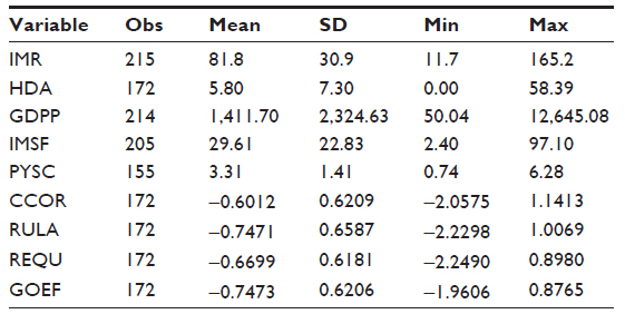Table 1 Health-related indicators across SSA (1990–2010) Abbreviations: CCOR, control of corruption; GDPP, per capita gross domestic product; GOEF, government effectiveness; HDA, health development assistance; IMR, infant mortality rate; IMSF, improved sanitation facilities; ln, natural log; Obs, observations; PYSC, primary years of schooling; REQU, regulatory quality; RULA, rule of law; SD, standard deviation; SSA, sub-Saharan Africa.

In the same year, Equatorial Guinea (−1.49), Democratic Republic of Congo (−1.42), Chad (−1.33), and Angola (−1.32) were found to show low performance in this indicator. On the basis of these governance indexes, in 2010, Botswana and Mauritius were found to exercise rule of law better than other countries 0.66 and 0.86, respectively. In the same year, these two countries showed better performance in government effectiveness as well – Botswana: 0.46; and Mauritius: 0.84. In contrast, this indicator was low in Comoros (−1.74), Democratic Republic of Congo (−1.73), and Equatorial Guinea (−1.7).

Estimation results and discussion

The estimation results from the three approaches are presented in Tables 2 and 3 as follows.

According to the identified estimator results in Table 2, except CCOR and REQU, all explanatory variables have coefficient estimates with the expected sign, negative. However, except ln GDPP, ln PYSC, and RULA, all the coefficient estimates were found to be statistically insignificant. Nonetheless, the insignificance may not necessarily be the reflection of the real image of the issue under consideration. Instead, it could be the distortion that might have arisen due to possible misspecification error committed in the form of omitted variables or wrong functional form.

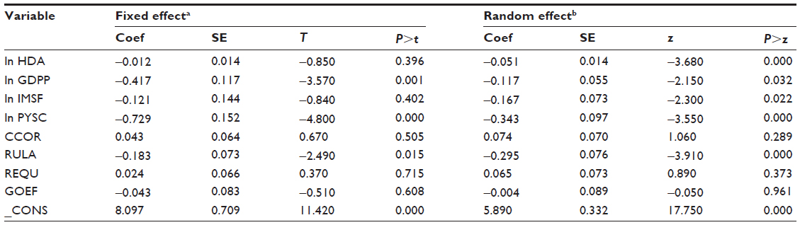Table 2 Estimates of IMR-estimating equation (1990–2010): results from fixed-effect and random-effect models Notes: Hausman test χ2(8)=41.53; P>χ2=0.0000. asigma_u=0.584; sigma_e=0.112; rho = 0.964; F(8,83)=29.05; P>F=0.0000. bsigma_u=0.206; sigma_e=0.112; rho = 0.772; Wald χ2(8)=186.72; P>χ2=0.000. Abbreviations: CCOR, control of corruption; Coef, coefficient; _CONS, constant; GDPP, per capita gross domestic product; GOEF, government effectiveness; HDA, health development assistance; IMR, infant mortality rate; IMSF, improved sanitation facilities; ln, natural log; P, probability; PYSC, primary years of schooling; REQU, regulatory quality; RULA, rule of law; SE, standard error; SSA, sub-Saharan Africa.

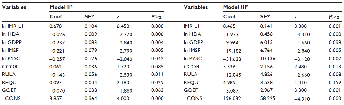Table 3 Estimates of IMR-estimating equation, 1990–2010: first-difference GMM results Notes: aArellano–Bond test for AR(1) in first differences: z=–0.272; P>z=0.786. Arellano–Bond test for AR(2) in first differences: z=–1.182; P>z=0.237. Wald χ2(9)=320.91; P>χ2=0.000; number of observations =91; number of instruments =39; correlation between predicted IMR and actual IMR =0.8395. bArellano–Bond test for AR(1) in first differences: z=–0.441; P>z=0.659. Arellano–Bond test for AR(2) in first differences: z=–1.012; P>z=0.312. Wald χ2(9)=527.13; P>χ2=0.000; number of observations =91; number of instruments =39; correlation between predicted IMR and actual IMR =0.8411. Abbreviations: AR(1), auto regressive order of 1; AR(2), auto regressive order of 2; CCOR, control of corruption; Coef, coefficient; _CONS, constant; GDPP, per capita gross domestic product; GMM, generalized method of moments; GOEF, government effectiveness; HDA, health development assistance; IMR, infant mortality rate; IMSF, improved sanitation facilities; ln, natural log; P, probability; PYSC, primary years of schooling; REQU, regulatory quality; RULA, rule of law; SE*, robust standard error.

The Hausman test presented at the bottom of Table 2 rejects the null hypothesis that states that the error terms are independent of the explanatory variables, which implies that the fixed-effect estimator is preferable to the random-effect one: χ²₍₈₎=41.53, P=0.000.

To refine the results more in this direction, we estimated Equation 15 and Equation 16 using first-difference GMM estimator and the estimation results are presented in Table 3.

Model II (left side of Table 3) reports that for the panel countries under consideration, the Arellano–Bond test for auto regressive of order 2 (AR(2)) in the first difference accepts the null hypothesis that states that the moment conditions are valid, which holds only if there is no serial correlation in the idiosyncratic errors. That is, the test confirms the hypothesis that the instrumental variables are acceptable because they fulfill the condition that they need not be correlated to the residuals. Moreover, the table reports that for these countries, the Wald test rejects the null hypothesis that states that all the coefficients except the constant term are zero. Furthermore, the table reports that the coefficient of the lagged dependent variable is 0.670, which is statistically significant: z=6.45; probability (Pr) >z=0.000. This suggests that in the estimation process of coefficient of ln HDA, unlike Model I, which assumes away the effect of lagged variables, controlling for previous level of IMR is necessary. Furthermore, the estimator gives −0.026 as the coefficient estimate of ln HDA, which is strongly significant: z=2.77; Pr >z=0.006, suggesting that, during the included period of study, HDA per capita has a statistically strong reducing effect on IMR. It indicates that in the region, a 1% increase in HDA reduces IMR by 2.6%. In other words, this result supports the belief that HDA has got a strong favorable effect in improving health status of the region. Similarly, the estimator gives −0.237 for ln GDPP, −0.221 for ln IMSF, and −0.257 for ln PYSC as the coefficient estimates, which are statistically significant (P=0.004, 0.005, and 0.042, respectively). These statistical test results suggest that improvement in income per capita, access to sanitation facilities, and undertaking primary education have strong effects in improving the health status of the region. Furthermore, the estimator gives −0.143 as the coefficient estimate of RULA, and this estimate is statistically significant (P=0.001), suggesting that strengthening rule of law has a strong favorable effect in the attempt to improve health status of the SSA region. Similarly, the estimator gives −0.07 as the coefficient estimate of GOEF, which is weakly significant (P=0.063), suggesting again that improving government effectiveness has some rewards in terms of improvement in health status in the SSA region.

A look at Model III estimation results conveys relatively similar messages. Table 3 (right side) indicates that the Arellano–Bond test for AR(2) in the first difference accepts the null hypothesis of no serial correlation in the idiosyncratic errors, which implies that the instrumental variables are acceptable: z=−1.012; Pr >z=0.312. Moreover, the table informs that for the panel economies under consideration, the Wald test rejects the null hypothesis that states that all the coefficients except the constant term are zero; χ²₍₉₎ =527.13; Pr >χ²=0.000. Just as in the case of Model II, the table reports that the coefficient of the lagged dependent variable is statistically significant: z=3.300; Pr >z=0.001, confirming the need for controlling for previous level of IMR in the estimation process of estimating the coefficient of ln HDA. That is, to be in the proximity of reality, the estimation procedure needs to include the previous level of IMR in the explanatory variables. Furthermore, the estimator gives −1.973 as the coefficient estimate of log-HDA, which is strongly significant: z=−4.31; Pr >z=0.000, implying, as in the case of Model II, that HDA has a strong negative effect on IMR. The estimate indicates that during the period of study covered, in the region, a 1% increase in HDA, which is far less than 10 cents per capita at the mean level, saves the life of two infants per 1,000 live births. This estimation result, again, strongly supports the view that in SSA, HDA has a strong effect in improving the health status of the population. On the other hand, the table indicates that the log-GDPP coefficient estimate is −9.96, which is significant at the 10% level of significance: z=−1.66; Pr >z=0.098, suggesting that raising per capita income growth contributes to the improvement of health status. In explicit terms, during 2001–2010, the IMR in SSA was 72 and per capita GDP growth was 2.0%. Keeping other variables unchanged, if in the subsequent periods, the region managed to raise the rate of growth to 3%, this would cause the IMR to fall to 62 infants per 1,000 live births.

In the same way, the estimator gives −19.18 as a coefficient estimate of ln IMSF, which again is statistically significant: z=−19.18; Pr >z=0.005. This estimation result implies that a 1% increase in access to improved sanitation facilities saves the life of 19 infants per 1,000 live births, confirming the strong impact that raising access to sanitation facilities has in enhancing the health status of the region. However, even if growth in IMSF has an impressive desirable effect on IMR, during the period of study, IMSF was exhibiting a declining rate, which may be due to the rising population. In such circumstances, keeping it from declining could be a hard task for the countries of the region. But should they be able to be in a position of raising the growth rate of this variable by 1%, they could reduce the regions’ IMR from 72, which was observed during 2001–2010, to 53 per 1,000 live births. The table also provides strong empirical evidence in support of the view that primary education has got a remarkable role in developing the health status. The estimation result indicates that a 1% increase in primary years of schooling could save the life of 32 infants per 1,000 live births. The estimate is statistically significant: z=−3.12; Pr >z=0.002. As in the case of Model II, the estimation results of Model III presented in Table 3 indicate that rule of law and government effectiveness indexes have negative and statistically significant coefficient estimates. This result points out the fact that in the region of study, good governance plays an impressive role in the endeavors made to improve health status.

The next issue is to point out which model (between Model II and Model III) fits better to the data of the region. From the results of Table 3, it is not so easy to indicate the preferable type. However, one can approach the question from a different angle. The correlation presented at the bottom of Table 3 indicates that both models have almost similar correlations between their predicted IMRs and actual IMRs; however, that of Model III is slightly greater. The other alternative is to look at the graphs of the actual IMR and the predicted IMR of the two models. Figure 1 presents the graph of the local polynomial smoothed line for actual IMR, predicted IMR from Model II, and predicted IMR from Model III for the included period of study, 1990–2010.

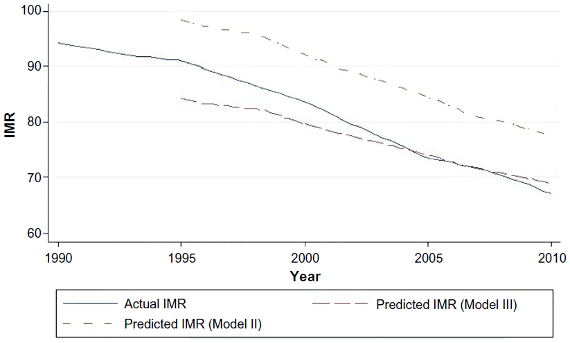Figure 1 Local polynomial smoothed line for IMR, 1990–2010. Abbreviation: IMR, infant mortality rate.

Figure 1 indicates that both the actual and the predicted IMRs were much greater than 80 per 1,000 live births in the early 1990s and exhibited a declining trend thereafter. Even if both models follow more or less the pattern that the actual IMR tracked, the predicted IMR from Model III is closer to the actual in level terms. Thus, here again, the less common (semilog) Model III seems to fit the data better than the more common (log-linear) Model II.

Finally, while the inclusion of ecosystem variables and demographic variables, such as immigration, could give better results, these limitations may be the basis for future research.

Summary and conclusion

This study, using IMR as a proxy for health status, has examined the effect of health development status on health based on a panel data set constructed from data on 43 sub-Saharan African countries from 1990 to 2010. Three equations used to estimate the IMR were proposed based on alternative assumptions. The first IMR-estimating equation assumes that the present level of IMR is determined solely by the present level of explanatory variables. It assumes the absence of lagged effects of explanatory variables as well as lagged effect of the IMR itself. This assumption, even though quite common in empirical works, is quite an oversimplification as the real situation involves lagged effects. In addition, the equation assumes the stability of elasticity of IMR with respect to explanatory variables. In this case again, even if the assumption is very common, it has no well-established explanation for the mechanism that ensures the assumed stability. The sign and significance of coefficient estimates obtained from this IMR-estimating equation were not plausible and hence the estimation results were not used for the inferences. The second IMR-estimating equation was based on the assumption that the present IMR depends partly on the previous level of IMR or lagged IMR, which after some mathematical manipulations could mean, in addition to the present level of all explanatory variables, the past levels of the explanatory variables have some influence on the present level of IMR, wherein their degree of influence decays with time. Moreover, this equation assumes the stability of IMR elasticity with respect to the explanatory variables. The equation was estimated using first-difference GMM. The estimation results obtained from this estimator were reported as competing results along with those of the third IMR-estimating equation. The third IMR-estimating equation assumes the presence of lagged effects but drops the assumption of stability of IMR elasticity with respect to explanatory variables. Instead, it assumes the stability of the product of the elasticities and IMR. That is, it considers rising elasticities, in absolute terms, as IMR falls with time. In this case again, first-difference GMM was used for estimating the IMR equation.

In the econometric analysis, per capita HDA, per capita income, primary years of schooling, improved sanitation facilities, CCOR index, rule of law index, REQU index, and government effectiveness index were used as the explanatory variables. The result obtained from the third IMR-estimating equation indicated that rule of law and government effectiveness have negative and statistically significant coefficients, suggesting that strengthening these two variables could serve as a useful measure in reducing the IMR of the region. Besides this, the estimation results suggested that strengthening participation in primary level education and provision of improved sanitation facilities have strong effects in reducing the IMR. Moreover, estimation of the third equation indicates that a 1% increase in per capita GDP will result in saving the life of ten infants per 1,000 live births. This result implies that to reduce the IMR by ten infants, per capita growth needs to be permanently raised sustainably by 1%. Concerning the variable of interest, HDA, the estimator gave negative and statistically significant coefficient estimates. It indicates that a 1% increase in per capita HDA growth would result in saving the life of two infants per 1,000 live births. Contrary to HDA pessimists’ view, this study observes the fact that HDA has strong favorable effect in improving health status of people in SSA.

We believe these findings add to the evidence in the scanty literature confirming a statistically significant and positive degree of interplay between health-targeted aid and health outcome in recipient countries. However, even if the positive impact of health-targeted aid is evidenced, SSA countries need to find ways of promoting domestic factors that have favorable impact on the health sector as they cannot rely upon external resources continuously for improving the health status of the population.

Disclosure

The authors report no conflicts of interest in this work.

---

References

1.	Bloom D, David C. The health and poverty of nations: from theory to practice. J Human Dev. 2003;4(1):47–71.
2.	WHO. Constitution of World Health Organization. Geneva: WHO; 1946.
3.	World Bank. World Development Indicators. Washington, DC: World Bank; 2011.
4.	Ravishankar N, Gubbins P, Cooley JR, et al. Financing of global health, tracking development assistance for health from 1990 to 2007. Lancet. 2009;373:2113–2124.
5.	Yogo UT, Mallaye D. Health Aid and Health Improvement in Sub-Saharan Africa: Accounting for the Heterogeneity Between Stable States and Post-Conflict States. J Int Dev. 2015;27(7):1178–1196.
6.	Levine R. Millions saved: proven successes in global health. In: Kinder M, editor. What Works Working Group. Washington, DC: Centre for Global Development; 2004:57–64.
7.	Ebeke C, Drabo A. Remittances, Public Health Spending and Foreign Aid in the Access to Health Care Services in Developing Countries. France: CERDI; 2011.
8.	Mishra P, Newhouse D. Does health aid matter? J Health Econ. 2009;28:855–872.
9.	Chauvet L, Gubert F, Mesple S. Aid, remittances, medical brain drain and child mortality: evidence using inter and intra-country data. J Dev Stud. 2013;49:801–818.
10.	Taylor ME, Hayman R, Crawford F, Jeffery P, Smith J. The impact of official development aid on maternal and reproductive health outcomes: a systematic review. PLoS One. 2013;8(2):e56271.
11.	Gormanee K, Girma S, Morrissey O. Aid, public spending and human welfare: evidence from quantile regressions. J Int Dev. 2005;17:299–309.
12.	Williamson CR. Foreign aid and human development, the impact of foreign aid to the health sector. South Econ J. 2008;75:188–207.
13.	Wilson S. Chasing success, health sector aid and mortality. World Dev. 2011;39:2032–2043.
14.	Wilson S, Gebhard NK, Kitterman KA, Mitchell A, Nielson D. The ineffectiveness of health sector foreign aid on infant and child mortality, 1975–2005”. Draft prepared for the Annual Meeting of the American Political Science Association; 2009; Boston.
15.	Baltagi BH. Econometric Analysis of Panel Data. 3rd ed. Hoboken, NJ: Johan Wiley and Sons Ltd; 2005.
16.	Arellano M, Bond S. Some tests for panel data: Monte Carlo evidence and an application to an employment equation. Rev Econ Stud. 1991;58:277–297.
17.	Blundell R, Bond S. GMM estimation with persistent panel data, an application to production functions. Econ Rev. 2000;19:321–340.
18.	Alonso-Borrego C, Arellano M. Symmetrically Normalized Instrumental Variable Estimation Using Panel Data. Abingdon: Taylor and Francis Ltd; 1999.
19.	World Health Organization [webpage on the Internet]. National Health Accounts. Geneva: WHO. Available from: http://www.who.int/nha. Accessed October 21, 2014.
20.	Barro R, Lee JW. A new data set of educational attainment in the world, 1950–2010. J Dev Econ. 2010;104:184–198.
21.	Maele NV, Evans D, Torres TT. Development assistance for health in Africa: are we telling the right story? Bull World Health Organ. 2013;91:483–490.
22.	Grépin KA, Kemon KL, Schneider M, Sridhar D. How to do (or not to do). Tracking data on development assistance for health. Health Policy Plan. 2012;27(6):527–534.
23.	World Bank [webpage on the Internet]. Worldwide Governance Indicators. Available from: http://data.worldbank.org/data-catalog/worldwide-governance-indicators. Accessed July 21, 2014.