Distinct patterns of corticogeniculate feedback to different layers of the lateral geniculate nucleus

Introduction

The principal gateway for retinal information to reach cortex is via the lateral geniculate nucleus (LGN) of the thalamus. One challenge to understanding LGN function is in understanding the significance of the massive recurrent pathway from primary visual cortex (V1) (for review see^1–3). A major issue is whether feedback pathways are arranged with the anatomical segregation seen in the feedforward pathways from the LGN to cortex. Such segregation would allow each pathway to be modulated independently by cortex. At the level of the LGN, only three primary channels – the magnocellular (M), parvocellular (P), and koniocellular (K) channels – have been recognized based on laminar arrangement, neurochemistry, and physiology.

Cortical feedback to the LGN arises entirely from cells in cortical layer 6 where retrograde bulk labeling evidence suggests that some segregation of corticogeniculate pathways may exist^4–6 (for review see Callaway⁷). In macaque monkey, cells in cortical layer 6A were reported to project to the LGN P layers (or neighboring K layers, K3–K6) while cells in 6B were reported to project primarily to the LGN M (or neighboring K layers, K1-K3).⁵ In bush babies, Conley and Raczkowski⁸ found that cells in the upper third of layer 6 projected to the P LGN layers and to LGN layer K4, cells in the middle and lower thirds of layer 6 projected separately to the M LGN layers and possibly neighboring K1–K3 LGN layers, while cells in the lower third of layer 6 projected to the pulvinar. Projections from a separate class of layer 6 cells that targeted the claustrum as well as other cortical areas (for review see Callaway⁷) were also found. Additional examination of the morphology of macaque layer 6 cells revealed that there are a number of different cells (see for review^9,10). No one to date, however, has shown whether distinct morphological classes of corticogeniculate cells send segregated feedback to the M, P, and K LGN layers. Regardless, in bush babies, macaque monkeys, and cats, physiological studies suggest that there exist at least three distinct feedback pathways based on speed of axonal conduction^11–13 (Casagrande and Norton, unpublished data, 1982). The latter results would support the hypothesis that the three main feedforward pathways to LGN from retina also get segregated feedback pathways from cortex. In owl monkeys, however, anatomical reconstructions of corticogeniculate axons support the hypothesis that feedback to P and M LGN cells is regulated separately, but that K LGN cells share feedback messages with pathways that innervate P cells or M cells, but not both.¹⁴

In light of the above information, our primary goal was to test whether the morphology of corticogeniculate cells and axons in bush babies supports the existence of two or three segregated feedback pathways to M, P, and K LGN cells. Conduction velocity data would support the existence of three feedback pathways whereas morphology of corticogeniculate axons in owl monkeys would argue for two feedback pathways^11,14 (Casagrande and Norton, unpublished data, 1982).

Materials and methods

Surgical procedures

Twenty-two bush babies (Otolemur garnettii), also known as greater galagos, were used in this study. Of these, ten were used for light microscopic reconstruction of corticogeniculate axons, eleven were used to analyze the morphology of corticogeniculate cells, and one was used to ultrastructurally examine the synaptic localization of labeled corticogeniculate axons in relationship to relay and interneuronal cell dendrites in LGN. These prosimian primates were young adults ranging in age from 10 months to 5 years. All of the animals were cared for according to the National Institutes of Health Guide for the Care and Use of Laboratory Animals and according to the guidelines of the Vanderbilt University Animal Care and Use Committee under an approved protocol.

All surgical procedures were carried out under aseptic conditions. Prior to surgery, animals were given cefazolin (25.0 mg/kg) to prevent surgical site infection, dexamethasone (2.0 mg/kg) to minimize swelling, glycopyrrolate (0.015 mg/kg) to minimize cardiodepressant effects, and cimetidine (5.0 mg/kg) to reduce gastric acid output. Animals were then intubated and anesthetized with 3%–4% isoflurane in oxygen. Anesthesia was maintained during surgery with the same gas mixture at 1%–2%. Heart rate, body temperature, and respiration rate were monitored throughout the procedure, and depth of anesthesia was additionally monitored by evaluating reaction to toe pinch. Anesthetic was increased as needed. Ophthalmic ointment (for cases involving injections into V1) or a thin film of silicone oil (for cases involving LGN recordings and injections) was placed on the corneal surfaces to prevent drying. Following stabilization, animals were secured in a stereotaxic apparatus. A midline incision was made in the skin and the muscle was retracted. Then, a craniotomy was made either over the LGN or over one or both hemispheres of V1. The dura was cut and retracted to expose the pial surface. Injections were made either in the lower layers of V1 or in individual layers of the LGN. To label corticogeniculate axons, pressure or iontophoretic injections (5 μA alternating current of 7 seconds on/ 7 seconds off for 20 minutes) of 5%–10% biotinylated dextran ([BDA] 3,000 molecular weight [MW]; Molecular Probes/Life Technologies, Thermo Fisher Scientific, Waltham, MA, USA) were made at depths ranging from 1–1.5 mm from the cortical surface. To label corticogeniculate cells, the LGN was located and the layers identified by recording visually evoked responses to a flashing light using a low impedance electrode (2 MΩ). Once the appropriate LGN layer was identified by ocular dominance shifts, the electrode was replaced with a glass pipette (20–30 μm tip diameter) containing either fluorescein isothiocyanate (FITC)–dextran or rhodamine isothiocyanate (RITC)–dextran (5% in 1 M KCl; 3,000 MW; Molecular Probes/Life Technologies, Thermo Fisher Scientific). The pipette was positioned in the layer of interest again on the basis of changes in eye dominance and the tracer was iontophoretically injected for 20 minutes (7 seconds on/7 seconds off, 5 μA).

After the injections were completed, artificial dura was placed over the exposed pial surface and the skin was sutured. Following extubation, the animals were given buprenorphine (0.01 mg/kg) to avoid pain. Animals were monitored closely until fully awake, eating, and drinking, and they were then returned to their home cages. Postsurgical monitoring was carried out to ensure the health and comfort of the animals.

Fixation and intracellular injections

After either 3–5 days (LGN injections) or 9–10 days (cortical injections), the animals were administered a lethal dose of sodium pentobarbital and were perfused transcardially with a saline rinse followed by a fixative. For the LGN injection cases, the fixative was 2% paraformaldehyde in 0.1 M phosphate buffer ([PB] pH 7.4); for the light microscopic cortical injection cases, the fixative contained 3% paraformaldehyde, 0.1% glutaraldehyde, and 0.2% saturated picric acid in 0.1 M PB (pH 7.4). The brain was blocked in the coronal plane with the head in a stereotaxic apparatus and the brain was then removed. In cases with cortical injections, brains were cryoprotected, allowing the tissue to equilibrate overnight in 30% sucrose in PB at room temperature. This tissue was then frozen on dry ice and stored until use at −70°C.

For the LGN injection cases, V1 was sectioned coronally with a Vibroslice (Campden Instruments Ltd, Loughborough, UK) into 300 μm thick slabs immediately after perfusion. The thick sections were collected in cold PB. Individual sections were examined for labeled cells in layer 6 under fluorescent illumination. When labeled cells were identified, the section was placed in a petri dish and secured in place with a piece of filter paper containing a small window that was placed over the area where the labeled cells were located. The filter paper was then weighted down and the dish was filled with cold PB. Sharp glass pipettes (tip diameter of approximately 1.0 μm) were used to make the injections. Cells were labeled with intracellular biotinylated Lucifer yellow (Thermo Fisher Scientific) (4% in H₂O) or biotinylated RITC–dextran (4% in saline). Injections were made by passing 10 nA of current through the pipette for 5–10 minutes. If the cell was filling well, filled dendrites with spines were typically visible within 2 minutes. Following the intracellular injections, sections were washed two times in cold PB and then placed in fixative (4% paraformaldehyde, 0.1% glutaraldehyde in PB) overnight at 4°C.

Histological procedures: light microscopy

After incubating overnight in fixative, sections with intracellularly injected cells were resectioned while frozen with a sliding microtome at 52 μm. The sections were equilibrated in 30% sucrose in PB for cryoprotection prior to resectioning. The sections were then frozen onto a layer of ice on the microtome stage and recut into 50 μm thick sections. These sections were collected in 0.1 M Tris buffered saline ([TBS] pH 7.4). Frozen sections through V1 of the cortically injected cases were cut coronally and the thalamus of both types of cases was cut parasagittally at 40–52 μm on a sliding microtome.

To visualize BDA, biotinylated Lucifer yellow and biotinylated RITC–dextran, sections were first treated with 10% methanol plus 0.3% H₂O₂ in 0.1 M TBS (pH 7.4) for 30 minutes at room temperature. Following three rinses in TBS, sections were placed in TBS plus 0.01% Triton X-100 with avidin biotin complex (Vector Elite; Vector Laboratories, Inc., Burlingame, CA, USA) for 2–12 hours at 4°C. The tissue was then rinsed three times in TBS and placed into a solution containing 50 mM TBS, 50 mM imidazole, 25 mM nickel ammonium sulfate, 0.25 mM 3, 3′-diaminobenzidine tetrahydrochloride hydrate (Sigma-Aldrich Co, St Louis, MO, USA), and 0.0003% H₂O₂. Sections remained in this solution until the reaction product became visible (15–30 minutes). The sections were then rinsed twice in TBS, mounted, air dried overnight, and coverslipped. To aid in analysis, sections also were counterstained with Giemsa (Sigma-Aldrich Co) to reveal the cell layers in the LGN and cortex. Giemsa counterstaining was carried out according to the protocol of Singleton and Casagrande.¹⁵

Axon data collection and analysis

Anterogradely filled corticogeniculate axons in the LGN were reconstructed from serial sections using a microscope with a camera lucida drawing tube. Only those cases in which the filling appeared complete (based on examination of axon structure at high magnification) were used for reconstruction and analysis. Cases were not used when the filling was patchy, granular, or very faint. Axons were selected for reconstruction only when that axon could be distinguished from the arbor of neighboring axons. Using these selection criteria, the entire axon arbor was traced to each terminal point in the LGN. Low-magnification drawings were used to orient and align adjacent sections using matching blood vessels and tissue elements. Lamination boundaries were indicated in the low-magnification drawings. Axons were then examined and traced at higher magnification (63× oil immersion objective) and these drawings were then aligned to reconstruct a complete 3D rendering of the axon in the environment of the tissue section translated to a 2D flat map.

Measurements of the maximum anterior/posterior axon extent were made to estimate the relative amount of visual field that was covered by individual axons and/or the entire column of axons in comparison to the known visuotopic map of bush baby LGN.¹¹ Measurements of individual axons were made after reconstruction at high resolution, and the axonal spread was measured relative to the most distal branches that had boutons along a plane parallel to the layer(s) in which the axon terminated, as originally defined in Ichida and Casagrande.¹⁴ The anterior/posterior extent of the anterograde column of labeling was identified with the camera lucida at the lowest resolution where the axons still could be easily distinguished and the whole column of label was visible in the field. Measurements were taken at the widest point of axonal spread, parallel to the layer, where the density of terminations fell off sharply; that is, the boundary of axonal distribution was placed at the ends of the most robustly ramifying axons. All sections containing a patch of anterograde labeling were reconstructed so that the label could be tracked as the position changed from section to section. This method allowed us to compare the extent of axonal label in different LGN layers.

The area of visual space that axons covered was estimated by converting the measurements of anterior/posterior extent into degrees and using the optic disc representation of Giemsa counterstained sections¹⁵ as a landmark. The map of the visual field in the bush baby LGN is organized, as in other primates, with the central vision representation posterior, peripheral vision representation anterior, upper visual quadrant lateral, and lower visual quadrant medial within the 3D map of LGN. The optic disc representation, identified histologically as a cell-free gap in the contralaterally innervated LGN layers, lies at 20° eccentricity (5° below the horizontal meridian representation). The portion of the LGN posterior to the optic disc representation was divided into three equal parts representing 0°–5°, 5°–10°, and 10°–20°. Thus, using the optic disc representation as a landmark, measurements of the label at its widest point in the anterior/posterior domain allowed us to estimate the relative amount of the visual field that was covered by either an individual axon or the column of axonal label.

Photomicrographs were taken with a Spot digital camera attached to an Olympus microscope (Olympus Corporation, Tokyo, Japan). Digital images were compiled in Adobe Photoshop (Adobe Systems Incorporated, San Jose, CA, USA).

Cortical cell reconstruction and analysis

Parts of injected cells found in sequential sections were reconstructed with the use of a camera lucida drawing tube at a final magnification of 600×. Once the full extent of the cell was reconstructed, the drawings from individual sections were compiled into a single image and stereological techniques were used to determine the relative amount of dendrite that individual cells extended into different layers of V1. These measurements were made using an isotropic uniform random test system of parallel lines.¹⁶ This system allows for the measurement of a curve in one plane. The estimate of length is based on the number of intersecting points that the curve makes with a known uniform random test system; in this case, a series of parallel lines at known and equal distances from each other. The number of intersections, along with the proper magnification factor and the distance between lines, can then be used to determine the length of the measured curve. This system assumes random, non-oriented placement of the uniform random test system with respect to the measured curve and an isotropic random orientation of the curve that is measured.

To verify the injection sites, digital images of the fluorescent injection sites were taken, and the sections containing these injections were counterstained for Nissl bodies using cresyl violet (Chroma-Gesellschaft Schmid GmbH & Co., Münster, Germany) and photographed again. Using these photographs, the LGN layer boundaries were traced in Adobe Photoshop and the resulting outline was overlaid on the matching individual fluorescent images of the injections sites.

Histological procedures: electron microscopy

The cortically injected animal used for electron microscopic analysis was sacrificed with a lethal dose of sodium pentobarbital and perfused transcardially with an oxygenated saline rinse followed by a fixative containing 3% paraformaldehyde and 1% glutaraldehyde in 0.1 M PB (pH 7.4). The brain was then removed and blocked parasagittally. Sections were cut through the LGN at 60–80 μm with a Vibroslice into cold PB. BDA was visualized with the same procedures used for light microscopy. Sections with label were incubated in 1% osmium for 1 hour at room temperature and rinsed three times in PB. Sections were then taken through a graded series of alcohols before being embedded in resin between ACLAR sheets (Ted Pella, Inc., Redding, CA, USA).

Once embedded, the tissue was examined at the light microscopic level, and a NeuroPunch (Ted Pella, Inc) was used to make 1.0 mm diameter punches of tissue which were restricted to M, P, or K layers. These tissue punches were mounted on resin blocks, and ultrathin sections (~70 nm) were cut with a diamond knife using an Ultracut E microtome (Reichert Life Sciences, Buffalo, NY, USA) and were then collected on uncoated 200-mesh nickel grids (Electron Microscopy Sciences, Hatfield, PA, USA).

Postembedding immunocytochemistry was then carried out to label for γ-Aminobutyric acid (GABA)-positive profiles. Ultrathin sections on grids were rinsed for 5 minutes in TBS with Triton-X ([TBST] 0.9% NaCl, 0.1% Triton X-100 in 0.05 M Tris, pH 7.6) and then incubated overnight with anti-GABA antibody (rabbit polyclonal; Sigma-Aldrich Co) diluted 1:20,000 in TBST (pH 7.6), followed by incubation in a goat anti-rabbit immunoglobulin (Ig)G conjugated to 30 nm gold particles (Ted Pella, Inc.) diluted 1:20 in TBST (pH 8.2) for 1 hour. After washing in deionized water, the sections were counterstained with uranyl acetate and lead citrate and examined using a Hitachi H-800 transmission electron microscope with an acceleration voltage of 100 kV (Hitachi High Technologies America, Inc, Dallas, TX, USA). As controls, sections were incubated in solutions omitting each step (primary and gold-conjugated secondary antibody) from the regular staining sequence, keeping the rest of the procedure the same as described. Control sections were totally devoid of gold particles.

Data collection and analysis: electron microscopy

Labeled corticogeniculate axon terminals (BDA positive) identified as making synaptic contact were analyzed in at least four different sections from each layer (M, P, or K). The total amount of tissue examined for each layer was 256,248 μm² for the M layers, 262,500 μm² for the P layers, and 250,000 μm² for the K layers taken from a series of sections from several blocks of tissue that were examined at 20,000×. GABAergic profiles typically contained many gold particles, but there was some background labeling. Here, we defined GABA profiles as those that contained two or more gold particles per 2.1±0.34 μm² of tissue. GABA-positive profiles in our samples contained a mean of ten gold particles ±1.8 per μm² of tissue. To estimate the level of background labeling, we took advantage of the fact that retinal terminals in the LGN have a distinct morphology at the electron microscopic (EM) level and are known to be glutamatergic.¹⁷ We measured the cross-sectional areas of recognizable retinal terminals and counted the number of gold particles within that area using unbiased morphometric procedures including randomized systematic sampling.¹⁶ These measurements yielded a very low background level of nonspecific labeling of one gold particle per 2.1±0.34 μm².

Data collection and analysis: statistics

Unless otherwise indicated above, all statistical comparisons were carried out using a Kruskal–Wallis one-way analysis of variance (ranked ANOVA) with a post hoc Mann–Whitney U pair-wise test corrected for three groups. The alpha level for significance was set at P≤0.05.

Results

The morphology of both corticogeniculate cell axons and their dendrites suggests that there are two different patterns of corticothalamic feedback: one set of pathways that relatively independently regulates P and M LGN input to cortex, and another that influences signals from all three pathways but principally targets the LGN K layers. The results presented below are divided into two sections. In the first major section, we describe and compare the morphology of corticogeniculate axons that terminate preferentially in P, M, or K LGN layers. In the second major section, we compare the dendritic morphology of cells projecting to the P and M layers with those that terminate in layer K4.

Corticogeniculate axon morphology

The injection sites in cortex were primarily confined within infragranular cortical layers, mainly layer 6 (Figure 1A). The cortical laminar designations are those described in Casagrande and Kaas,¹⁸ but a comparison with Brodmann’s¹⁹ terminology is given in the Figure 1 legend. LGN K layers were numbered, beginning at K1 between the contralaterally driven M layer and the optic tract. Both pressure and iontophoretic injections resulted in distinct columns of transported label in the LGN (Figure 1B, two fine arrows). Labeled axons were also observed in the thalamic reticular nucleus (TRN) and in the pulvinar (Figure 2). A total of 21 corticogeniculate axons were completely reconstructed using serial sections. These axons were very similar to corticogeniculate axons described in both owl monkeys¹⁴ and cats.²⁰ They were typically of very fine caliber with small en passant boutons, as well as terminal boutons at the ends of small stalks. Axons and boutons within the TRN and the pulvinar displayed a much more heterogeneous morphology. Unlike corticogeniculate boutons, TRN, and especially pulvinar boutons, varied widely in size and density (Figure 2). While there were some minor qualitative variations in axon diameter among corticogeniculate axons, no consistent variations were observed that could be correlated with LGN layer type (Figure 3).

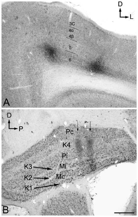Figure 1 Photomicrographs of two iontophoretic BDA injection sites. Notes: (A) Coronal section through the dorsal bank of V1. (B) The transported label in a parasagittal section through the LGN from the same case. The injections were centered in cortical layer 6 and confined to the infragranular layers of V1 (eg, layer 4 and 5). Here, we used cortical layer designations as follows with Brodmann’s19 terminology in parenthesis where it differs: 3C (4B), 4α (4Cα), 4β (4Cβ). The rationale for this choice is given in Casagrande and Kaas.18 The labeled axons in the LGN form two columns (arrows) that correspond to the pair of injections in layer 6 of V1. Numerals in LGN indicate different K layers. Scale bar =500 μm for (A) and (B). Abbreviations: BDA, biotinylated dextran; D, dorsal; K, koniocellular; L, lateral; LGN, lateral geniculate nucleus; Mc, contralateral magnocellular; Mi, ipsilateral magnocellular; P, posterior; Pc, contralateral parvocellular; Pi, ipsilateral parvocellular; V1, primary visual cortex.

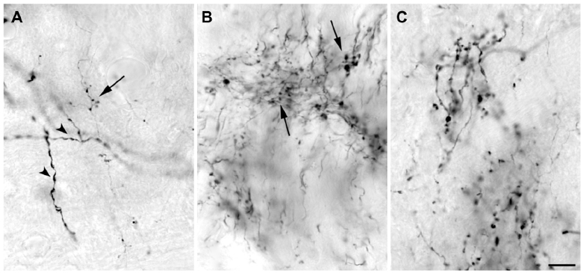Figure 2 High power photomicrographs of boutons labeled after injections into V1 that filled a small number of layer 6 cells. Notes: (A) LGN, (B) TRN, and (C) pulvinar. Terminations in the TRN are likely collaterals of axons that terminate in the adjacent LGN, but the pulvinar axons arise from separate cells. Arrowheads in (A) point to dendrites of a retrogradely filled cell in the LGN. Arrows in (A) and (B) compare bouton sizes on corticothalamic axons in the LGN and TRN, respectively. Scale bar =10 μm. Abbreviations: LGN, lateral geniculate nucleus; TRN, thalamic reticular nucleus.

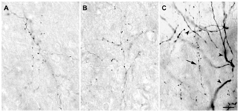Figure 3 High power photomicrographs of axons within the LGN. Notes: (A) P, (B) K, and (C) M layers. There was no qualitative difference in axon caliber or bouton size that correlated with LGN layer type. Corticogeniculate axons, arrow in (C), were much finer than geniculate relay cell dendrites (arrowheads). Scale bar =10 μm. Abbreviations: K, koniocellular; LGN, lateral geniculate nucleus; M, magnocellular; P, parvocellular.

Features of axons in M, P, and K layers

Several distinct patterns of corticogeniculate axons were found. No axons were reconstructed that terminated in both the M and the P layers. In contrast, every axon terminating in a K layer also sent branches that terminated in either a neighboring P layer or a neighboring M layer. No axons were found confined solely to a K layer, but some corticogeniculate axons were confined to single M or P layers, suggesting that they originated from monocularly driven cells in layer 6, as would be expected given physiological evidence that most cells in bush baby layer 6 have monocular receptive fields.²¹

Of the ten reconstructed axons that terminated in the M layers, two were restricted to the ipsilateral M layer, two were restricted to the contralateral M layer, and six had branches of similar density in both the ipsilateral and contralateral M layers. An example of one corticogeniculate M axon is shown in Figure 4 and a summary of the termination patterns of all ten corticogeniculate M axons is shown in Figure 5A. All of these axons had branches with boutons that extended into or through the neighboring K layers (K1, K2, and/or K3), shown in Figure 5 in red. The fact that K1, K2, and K3 are extremely narrow compared to K4 made it more challenging to determine whether axon branches existed that were confined to these K layers, but no changes in the branching patterns were seen as these axons traveled across laminar boundaries.

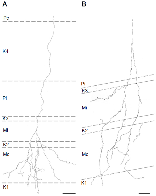Figure 4 Reconstructions showing corticogeniculate axon branching patterns in the M LGN layers. Notes: (A) An axon that innervated the M layer receiving input from the contralateral eye with branches in adjacent K layers K1 and K2. (B) Reconstruction of an axon that innervated both M layers with branches in K1, K2, and K3. Scale bars =50 μm. Abbreviations: K, koniocellular; LGN, lateral geniculate nucleus; M, magnocellular; Mc, contralateral magnocellular; Mi, ipsilateral magnocellular; Pc, contralateral parvocellular; Pi, ipsilateral parvocellular.

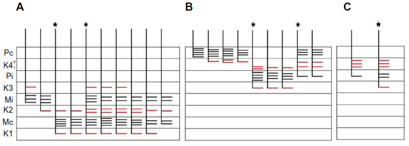Figure 5 Schematic diagrams summarizing the branching patterns of corticogeniculate axons. Notes: Corticogeniculate axons reconstructed in the (A) M layers (n=10), (B) P layers (n=9), and (C) K layers (n=2). The number and length of bars are not intended to represent exact branch length, but give a general idea of branch density within each LGN layer. The axons marked with a ⋆ are also shown in Figure 4 (A), Figure 6 (B) and Figure 7 (C). Branches that terminate in K layers for every axon are indicated in red. Abbreviations: K, koniocellular; Kci, koniocellular contralateral and ipsilateral portions of layer; LGN, lateral geniculate nucleus; M, magnocellular; Mc, contralateral magnocellular; Mi, ipsilateral magnocellular; P, parvocellular; Pc, contralateral parvocellular; Pi, ipsilateral parvocellular.

Of the nine axons with their main terminations in P layers, four innervated the contralateral P layer and three innervated the ipsilateral P layer. Two axons had branches in both the contralateral and ipsilateral P layers as well as in the intervening K layer (K4) (Figure 6). Three of the axons with branches in the contralateral P layer also had branches in K4, and all of the axons with branches in the ipsilateral P layer had branches in K4 as well as K3. Figure 5B shows a comparison of all nine patterns. In the bush baby, LGN K4 is subdivided into distinct sublayers that receive contralateral or ipsilateral retinal innervation, but not both.^22,23 The contralateral sublayer lies immediately ventral to the contralateral P layer while the ipsilateral sublayer lies just dorsal to the ipsilateral P layer.

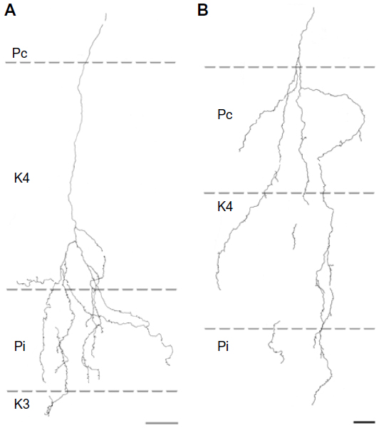Figure 6 Reconstructions showing corticogeniculate axon branching patterns in the P layers. Notes: (A) An axon that innervated the ipsilateral P layer with some branches in the ipsilateral portion of K4. (B) An axon that innervates both P layers along with all of K4. Scale bars =50 μm. Abbreviations: K, koniocellular; P, parvocellular; Pc, contralateral parvocellular; Pi, ipsilateral parvocellular.

Axons that innervated K4 along with an ipsilateral or contralateral P layer had their branches in K4 restricted to the portion of K4 that matched the eye dominance of the P layer that also received innervation (see Figure 6A). The two axons that innervated both P layers had branches with en passant boutons that were present throughout K4, thus innervating both contralateral and ipsilateral portions of that layer defined by ocular input (Figure 6B).

Two axons restricted the majority of their terminal branches to both sectors of the K4 layer, and had some branches that extended into the ipsilateral P layer (Figures 5 and 7). One of the axons also extended into K3.

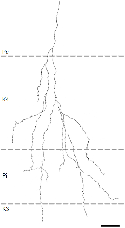Figure 7 Reconstruction of a corticogeniculate axon that innervated primarily K layers with branches in K4 and K3 as well as the ipsilateral P layer. Note: Scale bar =50 μm. Abbreviations: K, koniocellular; P, parvocellular; Pc, contralateral parvocellular; Pi, ipsilateral parvocellular.

Retinotopic distribution within the LGN

Individual axons extended 100–580 μm in the anterior–posterior dimension of the LGN, which would represent the peripheral to central regions of the bush baby visual field.²⁴ Axons located posterior to the optic disc representation (n=14) innervated a zone of cells representing 1.2°–7.3° of central vision (see Methods). Axons that innervated the M layers (n=5) covered a zone representing an average of 4.6°±0.6° (± standard error) of visual space, while P-layer axons (n=7) and K-layer axons (n=2) covered 3.3°±0.8° and 5.05°±0.05°, respectively. There was no significant difference in the extent of visual space covered by individual axons in different layers in this small sample (P>0.05). Measurements of the column of multi-axonal corticogeniculate label were made in two LGNs where the column of label was located in the representation of central vision posterior to the optic disc representation. Overall, the anterior–posterior width of the column of label in these two cases ranged from 136 to 620 μm, representing, on average, 4°±0.5° of visual space. The two cases did not differ significantly in the extent of axonal spread (P>0.05, Student’s t-test).

Synaptic contacts in the LGN

At the electron microscopic level, BDA-labeled corticogeniculate boutons were usually completely filled with dense and easily identifiable reaction product (see Figure 8). No labeled myelinated axons were observed. GABAergic profiles were clearly recognized by the presence of 30 nm gold particles, as exemplified by the large dendrite shown in Figure 8C. The level of background gold labeling was very low (see Methods).

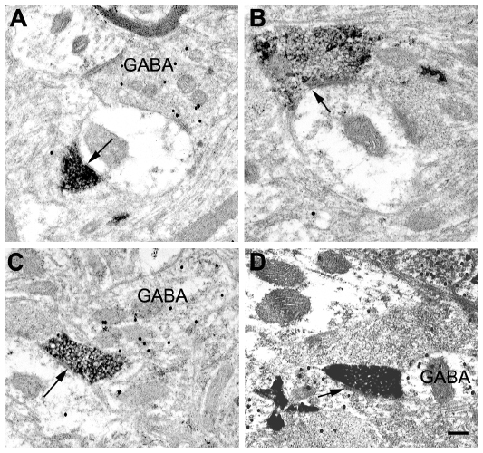Figure 8 Electron micrographs of BDA-labeled corticogeniculate terminals in the LGN. Notes: Labeled corticogeniculate terminals contain a dense black reaction product. Gold particles indicate the presence of GABA. (A) Labeled corticogeniculate terminal in a K layer making a synapse (arrow) onto an unlabeled (presumed glutamatergic) relay cell dendrite. (B) Labeled corticogeniculate terminal in an M layer with a synapse (arrow) on an unlabeled (presumed glutamatergic) dendrite, which received additional input from unlabeled terminal (on the right). (C) Labeled corticogeniculate terminal in a P layer with a synapse (arrow) on an unlabeled (presumed glutamatergic) dendrite. (D) An example of an infrequent corticogeniculate axon with a synapse (arrow) on a small GABAergic dendrite (GABA) in a P layer. Scale bar =0.2 μm. Abbreviations: BDA, biotinylated dextran; K, koniocellular; LGN, lateral geniculate nucleus; M, magnocellular; P, parvocellular; GABA, γ-Aminobutyric acid.

Corticogeniculate axons synapsed on unlabeled, presumably glutamatergic, dendrites in all LGN layers (Figure 8). Synapses with GABAergic dendrites were never observed in the M layers and only occasionally in the P and K layers (Figure 8D). In the M layers, 100% (n=16) of corticogeniculate terminals with unambiguous synapses terminated on unlabeled (glutamatergic) profiles. In the P layers, 78.6% (n=11) of corticogeniculate terminals with unambiguous synapses terminated on unlabeled (glutamatergic) profiles and 21.4% (n=3) synapsed onto GABAergic profiles. In the K layers, 93% (n=14) of corticogeniculate boutons synapsed with presumed glutamatergic profiles and 7% (n=1) synapsed with GABAergic profiles.

Corticogeniculate cell morphology

Injection sites and quality of intracellular filling

Injection sites were typically small (200–300 μm in diameter) and confined to the target LGN layers (Figure 9). Injections resulted in retrograde labeling of discrete patches of 5–8 cells within layer 6 of V1. Very often the shape of the cell body was clearly revealed by the retrograde labeling, making it easy to verify that the cell penetrated by the pipette was a labeled corticogeniculate cell. Cells were considered satisfactorily loaded with tracer if the apical and basal dendrites appeared completely stained and well-labeled to thin distal segments. Clear evidence of labeled spines both apically and basally was an important criterion. Figure 10A shows an example of a well-filled neuron, and the high power photomicrographs in Figures 10B and C confirm well-filled spines. This cell was unusual in that almost all of the apical dendrite was present in one 52 μm section. Typically, the apical dendrite had to be reconstructed through several serial sections. A total of 22 cells were satisfactorily filled and reconstructed to study feedback to each LGN layer class.

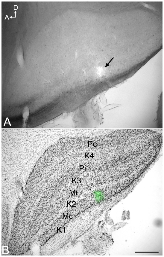Figure 9 Photomicrographs of an iontophoretic injection in the LGN and the same section Nissl stained to reveal the LGN layers. Notes: (A) Iontophoretic injection in the LGN. (B) The same section Nissl stained to reveal the LGN layers. The fluorescent injection site (arrow in [A] and green in [B]) is centered in the contralateral M layer. Scale bar =500 μm. Abbreviations: A, anterior; D, dorsal; K, koniocellular; LGN, lateral geniculate nucleus; M, magnocellular; Mc, contralateral magnocellular; Mi, ipsilateral magnocellular; Pc, contralateral parvocellular; Pi, ipsilateral parvocellular.

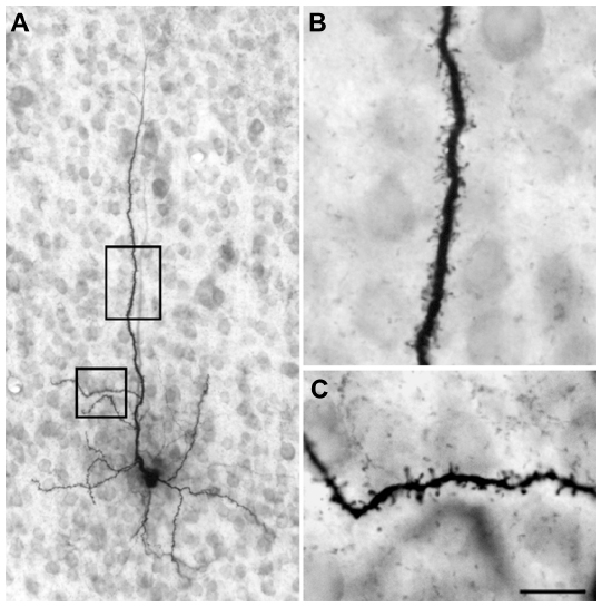Figure 10 Photomicrographs of an intracellularly filled cell in layer 6 of the primary visual cortex. Notes: (A) The cell body, many basal dendrites, and most of the apical dendrite are visible in this section. Scale bar =50 μm. (B and C) Higher power photomicrographs show well filled and easily distinguishable spines indicating that the filling was very complete. Scale bar =10 μm.

Morphological characteristics of corticothalamic neurons

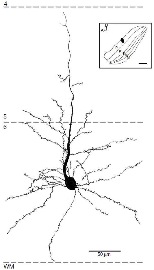
All reconstructed cells had similar pyramidal morphologies with basal dendrites ramifying within layer 6 and apical dendrites that extended superficially out of layer 6. All cells had at least part of their apical dendrite branches in layer 5. All of the cells that projected to K4 had dendrites in layer 4, while only one cell that projected to the M layers and two that projected to the P layers had apical branches that extended into layer 4. None of the cells had dendrites that extended above layer 4β, and the basal dendrites of most cells did not extend to the white matter or even to the bottom of layer 6B, but spread out more locally. Spines were present on apical and basal dendrites, but the number of spines decreased in the more distal dendritic branch segments. Thus, qualitatively, spines were concentrated in layers 6 and 5. Figures 11–13 show examples of filled cells from injections restricted to single LGN M, P, and K layers, respectively.

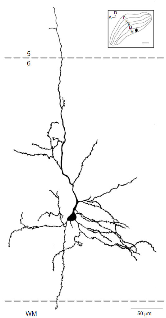Figure 11 Reconstruction of a corticogeniculate cell that was labeled following an injection into the M layers of the LGN. Notes: Most of this cell’s dendrites were restricted to layer 6. Only the apical dendrite extended beyond the layer 5/6 boundary. The inset shows the location of the injection site in the LGN. Scale bar =50 μm (500 μm in the inset). Abbreviations: A, anterior; D, dorsal; K, koniocellular; LGN, lateral geniculate nucleus; M, magnocellular; P, parvocellular; WM, white matter.

Figure 12 Reconstruction of a corticogeniculate cell that was labeled following an injection into the P layers of the LGN. Notes: The basal dendrites were arranged radially around the soma and were confined to layer 6. The apical dendrite extended up to the layer 4/5 boundary with branches in the upper part of layer 6 and a few sparse branches in layer 5. Scale bar =50 μm (500 μm in the inset). Abbreviations: A, anterior; D, dorsal; K, koniocellular; LGN, lateral geniculate nucleus; M, magnocellular; P, parvocellular; WM, white matter.

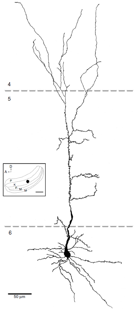Figure 13 Reconstruction of a corticogeniculate cell that was labeled following an injection into the K layers of the LGN. Notes: The basal dendrites were arranged radially around the soma and were confined to layer 6. The apical dendrite extended into layer 4 with branches in the upper part of layer 6, layer 5, and layer 4. Scale bar =50 μm (500 μm in the inset). Abbreviations: A, anterior; D, dorsal; K, koniocellular; LGN, lateral geniculate nucleus; M, magnocellular; P, parvocellular.

Seventeen cells had somas located in layer 6A; the somas of the remaining five were in layer 6B. None of the cells with somas in layer 6B projected to the main K layer: K4. In contrast, one-third of the cells projecting to the M layers (2/6) and P layers (3/9) originated in 6B. Because layer 6 varied greatly in width, the depth of individual cell somas was converted to a percentage of depth from the top of layer 6. Measurements made of cell-body location relative to the top of layer 6 showed that almost all cells were located in layer 6A. M-projecting cells (n=6) were located at an average of 41% depth from the top of layer 6, P-projecting cells (n=9) at 46%, and K4-projecting cells (n=7) were more superficial at 30%.

Corticogeniculate cells as a group showed restricted tangential spread of their dendrites, so each cell occupied less than half the width of a typical ocular dominance column in bush babies. M corticogeniculate cell dendrites covered, on average, 174±22 μm, P corticogeniculate cell dendrites 202±17 μm, and K corticogeniculate cell dendrites 191±25 μm.

Dendritic arborization patterns

Figure 14 shows schematic representations of all of the cells filled from injections into M, P, and K4 layers. In this figure, we have color coded cells whose dendrites extended into layer 4 where they were in a position to receive additional input directly from LGN axons that terminate in layer 4. In the case of the K-projecting cells, however, this input was always from one of the other pathways, M or P, and never in a closed loop from feedforward LGN K input, given that K feedforward axons terminate entirely above layer 4.

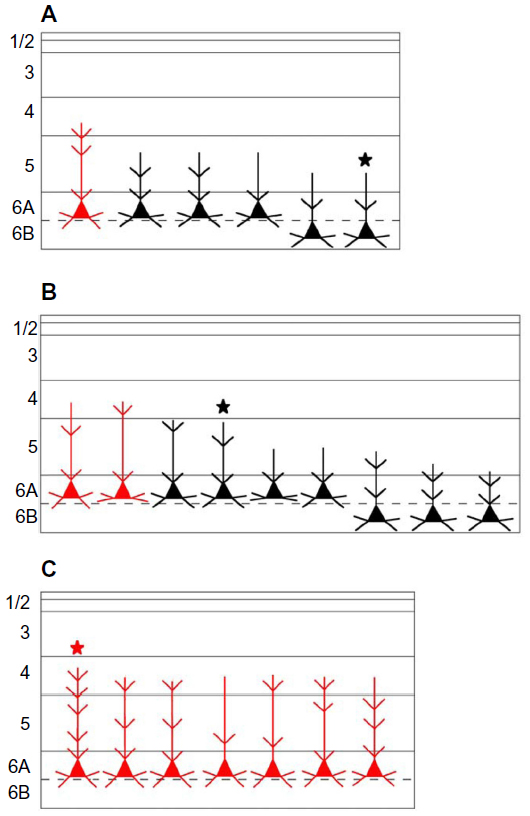Figure 14 Schematic diagram summarizing the dendritic arborizations of all filled and reconstructed cells. Notes: Filled and reconstructed cells projecting to (A) an M LGN layer, (B) a P LGN layer, or (C) K4. The number and length of the dendritic branches are not intended to represent the exact length, but to give a general idea of branch density within each cortical layer. Cells colored red are those with spines in cortical layer 4. Cells indicated by a ⋆ is also shown in Figure 11 (A), Figure 12 (B) and Figure 13 (C). Abbreviations: K, koniocellular; LGN, lateral geniculate nucleus; M, magnocellular; P, parvocellular.

In order to quantify these observations, we measured the total length of the dendritic tree that was present within each cortical layer (and subdivisions) for each cell (Figure 15). For convenience, these comparisons are shown as means ± standard error, but statistical comparisons were done against the median using a Kruskal–Wallis ANOVA and post hoc test (see Methods). M-projecting cells had an average total dendritic length of 1,785±106 μm, P-projecting cells had an average of 1,827±213 μm, and K4 projecting cells had an average of 1,768±332 μm. M, P, and K4 projecting cortical neurons did not differ in their total dendritic length measured across all layers (P>0.05, ANOVA).

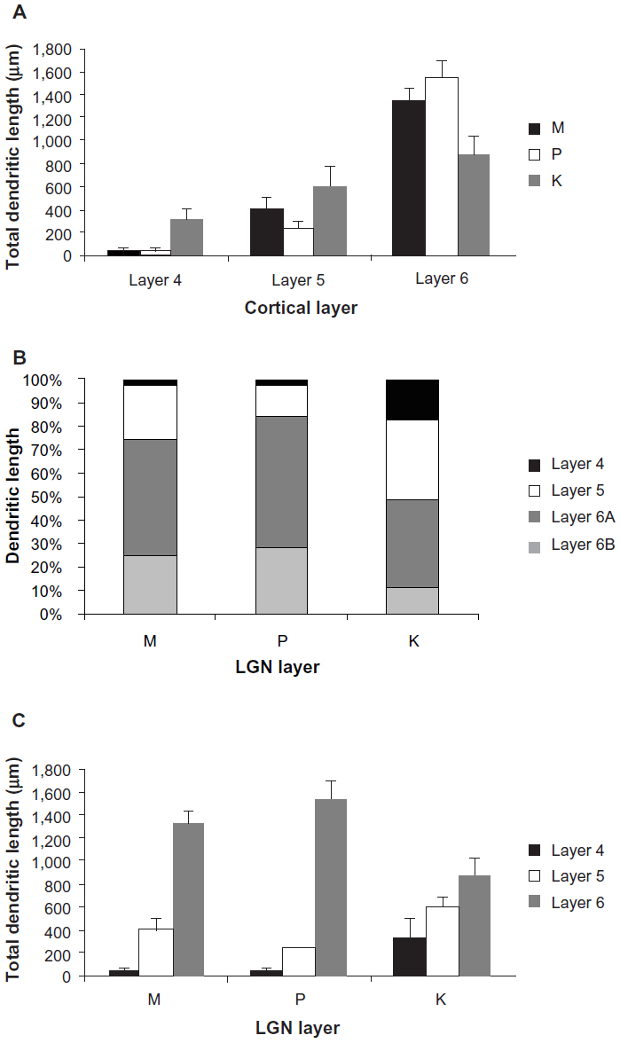Figure 15 Distributions of corticogeniculate cell dendrites. Notes: (A) Shows the distribution of dendrites per cortical layer. The majority of dendrites were located within layer 6. (B) Shows the percentage of dendritic length in each cortical layer for each corticogeniculate cell class. The distributions of dendrites is similar for M and P corticogeniculate cells and distinct from K corticogeniculate cells. (C) Shows the distribution of dendrites broken down by the LGN layer to which they project. K-projecting cells have a more even distribution of dendrites across layers 4, 5, and 6 with significantly more dendritic arbor in layer 4, while M- and P-projecting cells have the majority of their dendrites in layer 6. Abbreviations: K, koniocellular; LGN, lateral geniculate nucleus; M, magnocellular; P, parvocellular.

As shown in Figure 15A, the majority of dendrites for all corticogeniculate cells existed in layer 6. Comparisons revealed that layer 6 had significantly more total dendritic length than layer 5 (P=7×10⁻⁴) and layer 4 (P=1×10⁻⁶), and that more dendritic length was in layer 5 than layer 4 (P=0.01). Within layer 6 itself, analysis of dendritic length showed that dendrites remained local, as seen in Figure 15B. Thus, there were significantly more dendrites in 6A than in 6B collapsed across cell types (P=0.007). Within classes, this relationship was significant for cells projecting to LGN K4 and the P layers (P=0.007 and 0.03, respectively), but not significant for the cells projecting to the M layers. Finally, as shown in 15C, cells projecting to K4 stand out in comparison to cells projecting to the M and P layers as they have a much more even percentage of dendrites distributed across cortical layers and significantly more dendritic length in cortical layer 4. Only cortical layer 6 cells projecting to K4 showed no significant difference between the amount of dendrite contained in layer 4 compared to layer 5, or layer 5 compared to layer 6 (P>0.05). In contrast, 75% of M-projecting cell dendrites and 84% of P-projecting cell dendrites remained local within cortical layer 6.

Discussion

In this study, we asked whether corticogeniculate cells projecting to the M, P, and K LGN layers of the bush baby are morphologically distinct as might be predicted based on orthodromic conduction velocity differences identified originally (see Norton and Casagrande;¹¹ Casagrande and Norton, unpublished data, 1982) for axons projecting to these LGN layers. The answer is a qualified yes. Cells that send axons back to M or P LGN layers confine their dendrites primarily to cortical layer 6 and their axons to either M or P LGN layers, but not both. The latter cortical cell groups, however, can be further divided into subtypes. Some send axons that innervate only one monocular left or right eye LGN layer, some innervate both left and right eye LGN layers, and still others have variable lengths of axon that innervate more than one LGN cell class, either P and K or M and K. Cortical cells sending axons back to K LGN layers are the most distinct and heterogeneous as a group. These cells distribute their dendrites more evenly in cortical layers 5 and 6 and always extend distal branches into cortical layer 4. K corticogeniculate cells, unlike corticogeniculate P and M cells, never confine their axons to K LGN layers, but always distribute collaterals to either neighboring P or M layers.

Finally, our results show that corticogeniculate feedback is visuotopically matched between cortex and LGN, and that all feedback axons are extremely fine and primarily synapse on LGN relay cells regardless of layer rather than on GABAergic interneurons.

In the following discussion, we first consider some technical issues that must be kept in mind when interpreting these data and then consider the significance of these findings in light of prior work.

Technical considerations

When interpreting our results, it is important to be cognizant of a few technical limitations. One issue is whether axons or dendrites were completely filled, as is always a question in studies of this sort. Additionally, since cortical cells were filled in thick vibratome sections that were resectioned, one could question whether portions of dendrites were removed before filling. We believe this is unlikely for three reasons. First, cuts into the large apical trunk or the cell body generally result in the inability to fill the cell; instead, as one is attempting to fill the cells, a large fluorescent halo can appear, which often (although not always) suggests a leak. Second, we examined and selected cells to reconstruct that showed clear spines both apically and basally, as well as dense filling along all branches and branch segments. Finally, there were within-cell class consistencies that would be unlikely to occur if different parts of different cells were accidently removed in different cases. A second issue concerns the small sample size. Studies of the type described here are technically challenging because there are numerous details, from the original physiological identification of LGN layers to the final reconstructions of well-filled axons and dendrites, where problems can arise. Therefore, until other techniques are developed that would allow this type of analysis on a large scale in primates, all interpretation of the data must bear this caveat in mind.

Feedback axon patterns

The only other study of primate corticogeniculate axon morphology showed that, in owl monkeys, as in bush babies, feedback axons to the M and P LGN layers remain segregated while those innervating K layers always terminate either in neighboring M layers or P layers.¹⁴ Given the evolutionary distance between prosimians and simians,²⁵ such similarity suggests that this pattern applies broadly in primates. The fact that in both species some axons were found restricted to single P or M LGN layers also implies that feedback could influence individual monocular LGN layers independently. In bush babies, this possibility is supported by electrophysiological evidence showing that most (78%) of layer 6 corticothalamic neurons are monocular.²¹ While we can say that M and P layers receive segregated input, feedback to the K layers is more difficult to interpret. Only two out of 21 axons had the majority of their branches restricted to a K layer (ie, K4), but both exceptions still had branches in neighboring P layers. No evidence was found for axons specifically targeting layers K1–K3. One could argue that cortical input to K layers is specific at the synaptic level, but this observation does not match data showing that axons to K layers from the superior colliculus and retina in this species are tightly focused and limited even in the thin ventral K layers, implying that such laminar specificity can exist.²⁶

Input to K layers is complicated further by the fact that some K cells, defined by positive immunoreaction to the calcium-binding protein calbindin, are also loosely distributed in the M layers.²⁷ This finding implies that K and M cells share space in the M LGN layers and that, even if axons are targeted to specific K or M cells, they would appear anatomically indistinguishable at the light-microscopic level. Additionally, Feig and Harting²⁸ have shown that corticogeniculate axons terminate on the distal dendrites of bush baby LGN projection neurons, and since dendrites of M LGN cells (but not P LGN cells) extend into adjacent K-cell layers, cortical input could appear less segregated than it actually is at a single cell level.

An additional conundrum for all three corticogeniculate feedback pathways is the mismatch between aspects of their morphology and reported physiology. In bush babies, cats, and macaque monkeys, three distinct velocity groups have been identified that project to the M, P, and K layers (see^11–13,29; Casagrande and Norton, unpublished data, 1982), yet corticogeniculate axon reconstructions in bush babies, owl monkeys, and cats all report these axons to be fine (current work^14,20). However, the fact that the latter are all light-microscopic studies with small sample sizes would suggest that group differences could easily be missed and would require quantitative measurements at the EM level. In fact, inspection of the sizes of boutons (Figure 8) on corticogeniculate feedback axons certainly shows evidence of variation.

Our data show that the spread of cortical axons within individual layers of the LGN matches that which would be predicted given the receptive field sizes of layer 6 cortical cells in bush babies²¹ as well as the retinotopic map and magnification in individual LGN layers.³⁰ Similar results indicating that feedback axons are visuotopically precise in LGN have been reported for two other distantly related primates: the New World owl monkey¹⁴ and the Old World macaque monkey.³¹ Such results in primates contrast with those reported for cats where corticogeniculate axon extent was found to be much wider than the corresponding cortical layer 6 receptive fields would predict.²⁰ Taken together, these results imply that corticogeniculate feedback in primates, unlike in cats, more closely matches feedforward input. It is noteworthy, however, that TRN receptive fields are larger than LGN receptive fields,³² and collateral corticogeniculate branches to TRN still could provide a mechanism for selectively suppressing signals within the surrounding receptive field well beyond that which would be predicted based on cortical receptive field sizes of all species examined.^33,34

Corticogeniculate cells

Our laminar localization of corticogeniculate cell somas agrees with previously published data on bush babies.⁸ The latter results showed that most corticogeniculate cells were located in layer 6A with only a small percentage of corticogeniculate cells in 6B. In bush babies and other primates, layer 6A receives collateral branches from some LGN P cells, which would allow P cells to influence their own feedback as well as that of neighboring cells in LGN layer K4. All LGN M cell axons in bush babies have collateral branches in 6B where they could contact the basal dendrites of some corticogeniculate M cells as well as cortico-pulvinar cells located in the deepest part of layer 6B in VI.³⁵

Unlike M and P LGN cells, however, LGN K cells do not have collateral axon branches in layer 6 and so cannot close an auto-feedback loop; feedforward P and M axons can, however, potentially synapse on K feedback cells.^8,24,36

In macaques, layer 6 pyramidal cells have been subdivided into eight subclasses, only four of which showed evidence of axons in the white matter. This indicates that they project either subcortically (LGN, pulvinar), to claustrum, or to other cortical areas.^7,9,10 None of the layer 6 macaque projection neurons had dendritic arborizations that matched those we observed here in bush babies; all four potential corticogeniculate classes in macaques had dendrites that extended into layer 4.^9,10 There is a small chance that the difference is due to methodological differences, but we believe this is unlikely (see above). Additionally, we did find layer 4 distal dendrites arising from corticogeniculate K cells, but rarely from corticogeniculate M or P cells. These results provide argument for a genuine species difference between macaques and bush babies.

Functional aspects of corticogeniculate interactions

Many functions have been attributed to the massive corticogeniculate feedback pathways. We will not cover all of these proposals that include complex influences on spatial structure, length tuning, stimulus linked synchronization, binocular interactions including stereopsis and contrast gain control, etc (for review see^3,12,37). Instead, we highlight roles that can be correlated with our morphological observations. There are two ways to interpret the pathway differences observed in our data, summarized in Figure 16A and B. Figure 16A shows that corticogeniculate cells innervating the three main classes of LGN layers, M, P, and K, are morphologically distinct. This example is supported most strongly by the physiological data in macaque monkeys.²⁹ Figure 16B shows that both the feedforward and feedback pathways for the K channel share much less in common with the M and P channels than M and P channels share with each other, suggesting that there are primarily two types of feedback channels. The latter example is supported most strongly by anatomical data reported here for bush babies and previously for owl monkeys.¹⁴

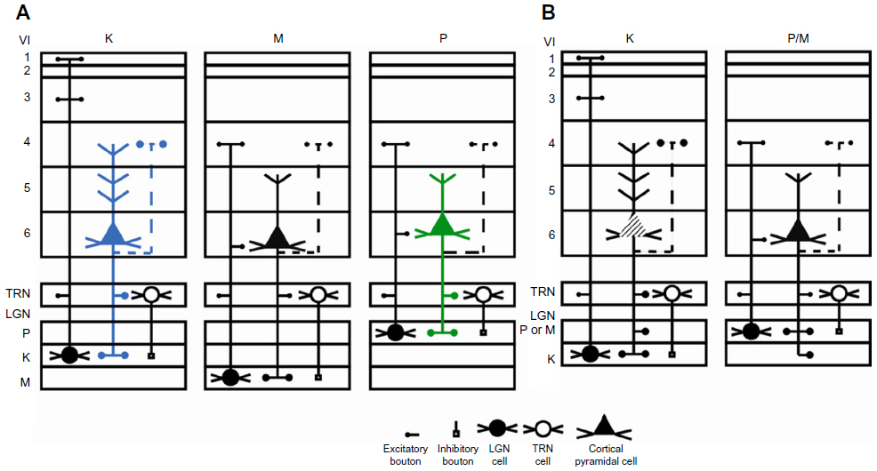Figure 16 Schematic diagram summarizing two interpretations of the main corticogeniculate pathways in primates. Notes: (A) Shows the three main pathways in the macaque monkey. The K pathway (blue) is shown on the left and represents only the blue on-portion of the K pathway based on a combination of anatomical and physiological data.12 The M pathway (black) is in the center and the P pathway (green) is on the right. (B) Compares the M and P pathways in bush babies and owl monkeys14 with the K pathway based primarily on anatomical data. The K pathway (striped) is shown on the left and the P/M pathways are shown on the right. Symbols below the figure identify different features. Arabic numerals refer to the V1 layers. Dotted lines indicate data either not shown or not part of this study but demonstrated in other studies. Abbreviations: K, koniocellular; LGN, lateral geniculate nucleus; M, magnocellular; P, parvocellular; TRN, thalamic reticular nucleus; V1, primary visual cortex.

The function of the corticogeniculate feedback pathway to K layers is potentially complex, given that it is in a position to provide a link between the different feedforward pathways both cortically and subcortically. Recent analyses of K-cell responses in marmosets indicate that they show oscillatory behavior that mirrors that seen in cortex.³⁸ This intriguing result hints that one role for the corticogeniculate K pathway(s) may be to synchronize activity depending on context or possibly shifts in attention. Evidence that corticogeniculate feedback could play a role in modulating the firing of LGN cells is provided by Sillito et al.³⁹ They showed that driving layer 6 cells with appropriately oriented moving bars synchronized the active cells in cat LGN. When activity was blocked in the visual cortex, the synchrony disappeared. The K pathway is in an ideal position to provide such temporal synchrony, given feedforward connections in layer 1 where the apical dendrites of the vast majority of pyramidal cells end in dendritic arborizations. These morphological observations also suggest testable hypotheses for future functional studies.

Although there is evidence for distinctions in morphology that correlate with layer 6 physiology,^40–44 the most relevant data here are data from Briggs and Usrey.²⁹ They provided evidence in macaque monkeys for a high degree of feedback specificity, particularly for feedback to macaque M cells (Figure 16A). Corticogeniculate cells targeting M cells showed a fast latency and exhibited transient responses and a low threshold for contrast typical of M LGN cells. These authors also showed evidence for another corticogeniculate population that shared characteristics with LGN P cells, and possibly also a third one, with blue on-responses characteristic of some K LGN cells. This form of specificity is suited to a role in locally enhancing or spatially highlighting specific classes of LGN cells. Such a role is also supported by results showing that corticogeniculate feedback enhances contrast gain in both macaque M and P cells,⁴⁵ and by our result showing that feedback axons primarily synapse on glutamatergic relay cells.

Acknowledgments

This work was supported by the National Eye Institute grant EY001778 (Casagrande), National Institute of Health core grants EY08126 and HD15051, and National Institute of Health training grant EY07135 (Ichida). Data analysis was performed in part through the use of the Vanderbilt University Medical Center Cell Imaging Shared Resource (supported by National Institute of Health grants CA68485, DK20593, DK58404, DK59637, and EY08126). The authors thank Dr Yuri Shostak for expert input to the electron microscopic data and analysis. The authors are also grateful to Drs Yuri Shostak, Gyula Sáry, Xiangmin Xu, David Royal, Ford Ebner, Roan Marion, and Keji Li for helpful comments on the manuscript, and Drs Sáry and Royal for help with some of the experiments. We are also grateful to Ashley Wenger for careful proofreading of our manuscript.

Disclosure

The authors report no conflicts of interest in this work.

---

References

1.	Sillito AM, Jones HE. Corticothalamic interactions in the transfer of visual information. Philos Trans R Soc Lond B Biol Sci. 2002;357(1428):1739–1752.
2.	Briggs F, Usrey WM. Corticogeniculate feedback and visual processing in the primate. J Physiol. 2011;589(Pt 1):33–40.
3.	Updyke BV. The patterns of projection of cortical areas 17, 18, and 19 onto the laminae of the dorsal lateral geniculate nucleus in the cat. J Comp Neurol. 1975;163(4):377–395.
4.	Wilson JR, Friedlander MJ, Sherman SM. Fine structural morphology of identified X- and Y-cells in the cat’s lateral geniculate nucleus. Proc R Soc Lond B Biol Sci. 1984;221(1225):411–436.
5.	Fitzpatrick D, Usrey WM, Schofield BR, Einstein G. The sublaminar organization of corticogeniculate neurons in layer 6 of macaque striate cortex. Vis Neurosci. 1994;11(2):307–315.
6.	Wilson JR, Forestner DM. Synaptic inputs to single neurons in the lateral geniculate nuclei of normal and monocularly deprived squirrel monkeys. J Comp Neurol. 1995;362(4):468–488.
7.	Callaway EM. Local circuits in primary visual cortex of the macaque monkey. Annu Rev Neurosci. 1998;21:47–74.
8.	Conley M, Raczkowski D. Sublaminar organization within layer VI of the striate cortex in Galago. J Comp Neurol. 1990;302(2):425–436.
9.	Wiser AK, Callaway EM. Contributions of individual layer 6 pyramidal neurons to local circuitry in macaque primary visual cortex. J Neurosci. 1996;16(8):2724–2739.
10.	Briggs F, Callaway EM. Layer-specific input to distinct cell types in layer 6 of monkey primary visual cortex. J Neurosci. 2001;21(10):3600–3608.
11.	Norton TT, Casagrande VA. Laminar organization of receptive-field properties in lateral geniculate nucleus of bush baby (Galago crassicaudatus). J Neurophysiol. 1982;47(4):715–741.
12.	Briggs F, Usrey WM. Parallel processing in the corticogeniculate pathway of the macaque monkey. Neuron. 2009;62(1):135–146.
13.	Tsumoto T, Suda K. Three groups of cortico-geniculate neurons and their distribution in binocular and monocular segments of cat striate cortex. J Comp Neurol. 1980;193(1):223–236.
14.	Ichida JM, Casagrande VA. Organization of the feedback pathway from striate cortex (V1) to the lateral geniculate nucleus (LGN) in the owl monkey (Aotus trivirgatus). J Comp Neurol. 2002;454(3):272–283.
15.	Singleton CD, Casagrande VA. A reliable and sensitive method for fluorescent photoconversion. J Neurosci Methods. 1996;64(1):47–54.
16.	Cruz-Orive LM, Weibel ER. Sampling designs for stereology. J Microsc. 1981;122(Pt 3):235–257.
17.	Guillery RW. A study of Golgi preparations from the dorsal lateral geniculate nucleus of the adult cat. J Comp Neurol. 1966;128(1):21–50.
18.	Casagrande VA, Kaas JH. The afferant, intrinsic, and efferent connections of primary visual cortex in primates. In: Peters A, Rockland KS, editors. Primary Visual Cortex of Primates. Cerebral Cortex. Vol 10. New York: Plenum; 1994:201–259.
19.	Brodmann K. Localization in the Cerebral Cortex. Leipzig: Johann Ambrosius Barth; 1909.
20.	Murphy PC, Sillito AM. Functional morphology of the feedback pathway from area 17 of the cat visual cortex to the lateral geniculate nucleus. J Neurosci. 1996;16(3):1180–1192.
21.	DeBruyn EJ, Casagrande VA, Beck PD, Bonds AB. Visual resolution and sensitivity of single cells in the primary visual cortex (V1) of a nocturnal primate (bush baby): correlations with cortical layers and cytochrome oxidase patterns. J Neurophysiol. 1993;69(1):3–18.
22.	Kaas JH, Huerta MF, Weber JT, Harting JK. Patterns of retinal terminations and laminar organization of the lateral geniculate nucleus of primates. J Comp Neurol. 1978;182(3):517–553.
23.	Casagrande VA, Joseph R. Morphological effects of monocular deprivation and recovery on the dorsal lateral geniculate nucleus in galago. J Comp Neurol. 1980;194(2):413–426.
24.	Ding Y, Casagrande VA. The distribution and morphology of LGN K pathway axons within the layers and CO blobs of owl monkey V1. Vis Neurosci. 1997;14(4):691–704.
25.	Seiffert ER, Simons EL, Clyde WC, et al. Basal anthropoids from Egypt and the antiquity of Africa’s higher primate radiation. Science. 2005;310(5746):300–304.
26.	Lachica EA, Casagrande VA. The morphology of collicular and retinal axons ending on small relay (W-like) cells of the primate lateral geniculate nucleus. Vis Neurosci. 1993;10(3):403–418.
27.	Johnson JK, Casagrande VA. Distribution of calcium-binding proteins within the parallel visual pathways of a primate (Galago crassicaudatus). J Comp Neurol. 1995;356(2):238–260.
28.	Feig S, Harting JK. Ultrastructural studies of the primate lateral geniculate nucleus: morphology and spatial relationships of axon terminals arising from the retina, visual cortex (area 17), superior colliculus, parabigeminal nucleus, and pretectum of Galago crassicaudatus. J Comp Neurol. 1994;343(1):17–34.
29.	Briggs F, Usrey WM. A fast, reciprocal pathway between the lateral geniculate nucleus and visual cortex in the macaque monkey. J Neurosci. 2007;27(20):5431–5436.
30.	Casagrande VA, Norton TT. The lateral geniculate nucleus: A review of its physiology and function. In: Leventhal AG, editor. The Neural Basis of Visual Function. London: MacMillan Press; 1991;4:41–84.
31.	Angelucci A, Sainsbury K. Contribution of feedforward thalamic afferents and corticogeniculate feedback to the spatial summation area of macaque V1 and LGN. J Comp Neurol. 2006;498(3):330–351.
32.	Funke K, Eysel UT. Inverse correlation of firing patterns of single topographically matched perigeniculate neurons and cat dorsal lateral geniculate relay cells. Vis Neurosci. 1998;15(4):711–729.
33.	Webb BS, Tinsley CJ, Barraclough NE, Easton A, Parker A, Derrington AM. Feedback from V1 and inhibition from beyond the classical receptive field modulates the responses of neurons in the primate lateral geniculate nucleus. Vis Neurosci. 2002;19(5):583–592.
34.	Alitto HJ, Usrey WM. Origin and dynamics of extraclassical suppression in the lateral geniculate nucleus of the macaque monkey. Neuron. 2008;57(1):135–146.
35.	Florence SL, Casagrande VA. Organization of individual afferent axons in layer IV of striate cortex in a primate. J Neurosci. 1987;7(12):3850–3868.
36.	Lachica EA, Casagrande VA. Direct W-like geniculate projections to the cytochrome oxidase (CO) blobs in primate visual cortex: axon morphology. J Comp Neurol. 1992;319(1):141–158.
37.	Cudeiro J, Sillito AM. Spatial frequency tuning of orientation-discontinuity-sensitive corticofugal feedback to the cat lateral geniculate nucleus. J Physiol. 1996;490(Pt 2):481–492.
38.	Cheong SK, Tailby C, Martin PR, Levitt JB, Solomon SG. Slow intrinsic rhythm in the koniocellular visual pathway. Proc Natl Acad Sci. 2011;108(35):14659–14663.
39.	Sillito AM, Jones HE, Gerstein GL, West DC. Feature-linked synchronization of thalamic relay cell firing induced by feedback from the visual cortex. Nature. 1994;369(6480):479–482.
40.	Gilbert CD, Wiesel TN. Morphology and intracortical projections of functionally characterised neurones in the cat visual cortex. Nature. 1979;280(5718):120–125.
41.	Martin K, Whitteridge D. The relationship of receptive field properties to the dendritic shape of neurones in the cat striate cortex. J Physiol. 1984;356(1):291–302.
42.	Anderson JC, Martin KA, Whitteridge D. Form, function, and intracortical projections of neurons in the striate cortex of the monkey Macacus nemestrinus. Cereb Cortex. 1993;3(5):412–420.
43.	Hirsch JA, Alonso JM, Reid RC, Martinez LM. Synaptic integration in striate cortical simple cells. J Neurosci. 1998;18(22):9517–9528.
44.	Steriade M. Coherent oscillations and short-term plasticity in corticothalamic networks. Trends Neurosci. 1999;22(8):337–345.
45.	Uhlrich DJ, Cucchiaro JB, Humphrey AL, Sherman SM. Morphology and axonal projection patterns of individual neurons in the cat perigeniculate nucleus. J Neurophysiol. 1991;65(6):1528–1541.