Deep Learning for the Automatic Diagnosis and Analysis of Bone Metastasis on Bone Scintigrams

Introduction

Bone scintigraphy with ^99mTc-methylene diphosphonate (MDP) has been widely used to detect BMs of malignant tumors and to evaluate the effect of treatment. With the increase in the incidence of domestic tumors such as breast cancer, prostate cancer, pulmonary cancer and so on, the examination requirements for bone scintigraphy have also increased. A report from the Chinese national survey of nuclear medicine showed that bone scintigraphy ranked first in the total number of single-photon examinations in 2019, accounting for 63.1%.¹ The task of manually interpreting images is demanding and tedious. As doctors become more fatigued, misdiagnosis can easily occur. In addition, the interpretation of bone scan images depends on the personal knowledge and experience of nuclear medicine physicians.

At present, an increasing number of computer-assisted diagnosis (CAD) systems^2–7 have been employed to detect bone diseases on bone scintigraphy. Most of these methods aim to extract the radioactivity accumulation areas on the images using the threshold-based approach and to judge a single hot zone or an entire image by inputting the manually extracted imaging features into a simple multilayer fully connected network, which can hardly cover all the information on the image. In recent years, deep learning has witnessed dramatic progress in the analysis of many medical images, such as CT, MRI, and this method mainly focuses on image segmentation, the extraction and classification of imaging features and target detection, such as for lung nodule detection⁸ and liver tumor segmentation.⁹ In terms of BM, Chmelik¹⁰ used a CAD system based on voxel-based classification convolutional neural network (CNN) to segment the entire spine on sagittal CT images of 1046 osteolytic lesions and 1135 osteogenic lesions from 31 patients. The presence or absence of BM within each tissue voxel was determined. Of the 24,000 segmented tissue voxels in the test set, the AUC of the model for identifying the osteolytic lesions was 0.80, and the AUC of osteogenic lesions was 0.72. The sensitivity for localizing small bone lesions less than 1.5mm in diameter and large bone lesions more than 3cm in diameter were 92% and 99% respectively. Wang’s team¹¹ also employed a classification CNN model to analyze the BMs on the nonsegmented sagittal fat-suppressed T2-weighted 2D FSE images of the spine from 26 patients. The model had the sensitivity of 90% for localizing the bone lesions. However, whether it is CT or MRI, it is difficult to detect and assess the whole-body bone metastatic lesions, but bone scintigraphy could. To the best of our knowledge, few studies have been conducted on the application of deep learning in interpreting bone scintigrams. Papandrianos¹² used a fast CNN architecture to differentiate a BM case from other either degenerative changes or normal tissue cases with a high accuracy of 91.61%±2.46% on whole-body scintigraphy images for prostate patients. Additionally, the author also compared his method to other popular CNN architectures, such as ResNet50, VGG16, GoogleNet and MobileNet, and achieved superior performance. Pi¹³ reported an accuracy of 94.19% for automated diagnosis of BM based on multi-view bone scans using attention-augmented deep neural networks, and his datasets were from more than ten thousand of examinations with different primary tumors. Han¹⁴ has built two different 2D CNN architectures (whole-body-based and tandem architectures integrating whole body and local subimages), the later performed better with an accuracy of 0.900. The disadvantages of all above literatures were either limited to one primary tumor or a limited amount of data, and most of their studies were about classification, they have not extended to the segmentation, even to other analysis.

In the past few decades, to evaluate the effect of therapy on malignant tumors more objectively, different imaging-based evaluation criteria have emerged. Tumor burden is thought to reflect the therapeutic effect. Initially, its evaluation solely relies on tumor size,^15,16 now, tumor metabolic indicators or immune detection have been emerged.^17–19 However, bone lesions have been regarded as nonmeasurable lesions in the current evaluation criteria, making it difficult for clinicians to employ quantitative and objective criteria to evaluate tumor burden of bone lesions.

The highlight of our study was that we proposed a robust deep learning framework for automatic BM interpretation. This deep learning technology can extract features of metastatic bone lesions from bone scintigrams, perform image classification and segmentation, and automatically generate primary reports. Especially, we also attempted to calculate the overall tumor burden of all automatically identified bone lesions to evaluate the effects of therapy on BMs.

Materials and Methods

Patients

A total of 1373 bone scintigrams were retrospectively identified from the Department of Nuclear Medicine, Tenth People’s Hospital of Tongji University from March 2018 to July 2019. Based on previous clinical reports, a nuclear medicine physician with over 10 years of experience reviewed the images and their clinical histories, then divided them into two groups: the BMs group and the non-BMs group, which were regarded as golden standard. The inclusion criteria were as follows: 1) BMs group, with a history of malignant tumor, appeared as abnormal accumulation of MDP on bone scan images, and were confirmed by CT, MRI, biopsy or follow-up and 2) non-BMs indicated no MDP uptake suggesting bone metastasis, regardless of the presence of MDP uptake considered as unlikely for bone metastasis, such as the joints or spine of patients with degenerative diseases, areas of trauma, postoperative regions, areas of osteoporosis and so on, then with 6 months follow-up, bone lesions improved without progression. The exclusion criteria were as follows: 1) primary bone tumors; 2) bone lesions that were not confirmed; and 3) BMs only manifested as radioactive defects on bone scan image.

Peripheral blood alkaline phosphatase²⁰ (ALP) which is generally investigated as a clinically validated indicator for BMs was also adopted in this study. The inclusion criteria for the verification patients were as follows: 1) patients with tumors were diagnosed with BMs at the first time and 2) within 2 weeks before and after bone scintigraphy, all patients underwent the ALP test before treatment. The exclusion criteria were as follows: 1) hepatobiliary disorders; 2) previous treatment; 3) thyroid diseases, diabetes, rheumatism, etc; 4) medication with drugs, such as hormones and bisphosphonates, within 3 months, which may affect bone metabolism; and 5) traumatic fracture within 1 year or metabolic bone diseases.

Bone Scans

The patients underwent whole-body bone scans 2–3 h after intravenous administration of ^99mTc-MDP (370–740 MBq). All acquisitions were performed with a GE Discovery NM/CT 670 (GE, USA) equipped with low-energy, high-resolution collimators (10% window width, peak energy 140 keV, and 256×1024 matrix). Standard whole-body anterior and posterior sweep images were acquired with a scan speed of 10–20 cm/min. The imaging processing systems were from GE Medical Systems.

Methods

Generally, the model cannot be properly optimized but can obtain good evaluation results when the segmentation dataset is extremely unbalanced. For example, a single-category segmentation dataset only 20% of the data contains the ROI area, the Dice score can still reach 0.8 when the model predicts all the results as the background area. To this end, we designed a stepwise segmentation framework to optimize the model reasonably.

The overall framework is illustrated in Figure 1. Firstly, cropping the whole-body bone scan image into sub-images. Secondly, putting sub-image to diagnostic classification model determines whether it contains the region of interest. When the region of interest is included, the sub-image is input into the segmentation model to obtain the diseased segmentation map, and when the region of interest is not included, the normal segmentation map is directly obtained. Thirdly, input both whole-body bone scan and whole-body segmentation map into diagnostic report generation model generate the diagnostic report, which includes the tumor burden and the location of region of interest. Specifically, the classification, segmentation and report generation models are trained separately. The details of the framework are outlined below.

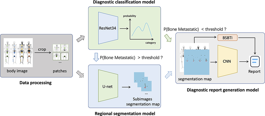Figure 1 Overall architecture of the prediction framework. First, the original images are cropped into subimages. Then, each subimage first uses the region classification model to determine whether the area contains tumors or bladder. If it contains bone metastases or bladder, the data is input to the area segmentation model to obtain the segmentation result. The full image segmentation result is generated by combining the subimage segmentation results. Finally, the original image and the segmented image are concatenated together, and a model is generated through a diagnostic report to obtain a final report.

Data Processing

The original data contained the anterior and posterior images with two different gray values (Figure 2A). The areas of the BMs and bladder were outlined by Labelme²¹ (Figure 2B). The original image size was not fixed. The image size was resized to 1024×1024 with bilinear interpolation, and then the labels were interpolated to the same size by using nearest neighbor interpolation to adapt to the network input. The data were divided into seven levels according to the pixel values, which were counted by the labeled results: zero-pixel level, single-pixel level, ten-pixel level, hundred-pixel level, thousand-pixel level, mega-pixel level, and 100,000-pixel level. Eighty percent of the data at each level were randomly selected as the training set and validation set, and the remaining 20% was used as the testing set.

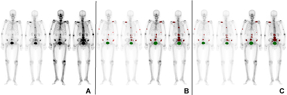Figure 2 Results of data synthesis. (A) Original bone scan image; (B) Manually labeled bone scan image; (C) Model prediction result. The red area represents bone metastases, and the green area represents the bladder.

All models in this study used the same hardware configuration (GPU is 1080Ti, and the CPU model is E5-2697). We used the Pytorch framework and Adam optimizer during training. The initial learning rate was 0.01, and the batch size was set to 16.

Diagnostic Classification Model

The diagnostic classification model aimed to determine whether the input image contained BMs or bladder.

Data Processing

To retain the original information of the image as much as possible, the model used the subimage with a size of 256×256 as input. The image was sampled from the original image with a sliding window of 128 steps. Thus, one image with a size of 1024×1024 could obtain 28 subimages with sizes of 256×256. The classification labels are two-dimensional vectors, in which two elements represent whether the data contain BMs and bladder. The diagnostic classification model was trained by subimages and corresponding classification labels.

Model Structure

ResNet34 architecture was used as the diagnostic classification model. To adapt to single-channel grayscale data and data size, the average pooled convolution kernel of the first layer and the last layer was increased to 8 × 8, and the output size of the last fully connected layer was adjusted to 2, corresponding to the two-class classification probability (metastases and bladder). The modified model structure is shown in Table 1. We refer readers to ref²² for a more detailed formulation of the residual structure. The model is initialized with ImageNet pre-training parameters.

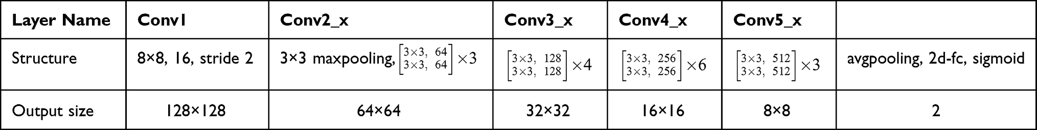Table 1 The Network Structure of the Diagnostic Classification Model

In our experiments, focal loss²³ was used as the loss function in the classification diagnosis model and was mainly used to address the issue of classification imbalance. A dynamic scaling factor γ was added based on the cross-entropy loss to automatically reduce the loss of simple samples and help the model train difficult samples. In this study, γ= 1, and the diagnosis model was trained with the SGD (stochastic gradient descent) optimizer. The formula is as follows:

where are category tags, and are the probabilities that the model outputs 1.

Regional Segmentation Model

The segmentation model aims to segment the BM tumor area and the bladder area at the pixel level.

Data Processing

Based on the data obtained by sliding windows, the data containing BMs or bladder were screened to train the BM segmentation model or bladder segmentation model. Random rotation, scaling, and flipping were used for data augmentation.

Model Structure

To accelerate model convergence and improve segmentation accuracy, the U-net²⁴ encoding and decoding structures were adopted. The network consists of convolutional blocks. Each convolutional block consists of 3×3 convolutional layers, batch normalization, and Leaky rectified linear units (Leaky ReLU). A 1×1 convolution residual structure was introduced into each convolution block to accelerate convergence. At the same time, the convolution block can change the number of channels in the feature map. The structure of the region segmentation model is shown in Figure 3. The model is initialized with ImageNet pre-training parameters.

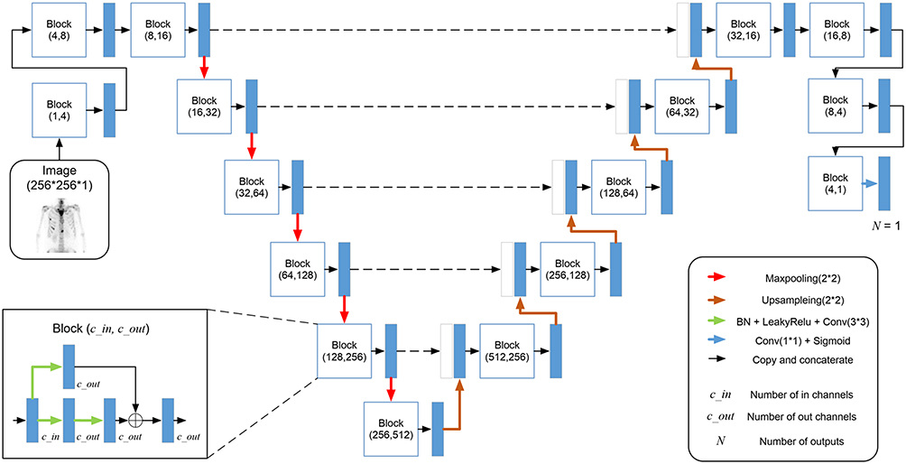Figure 3 Region segmentation network structure. Blue and white boxes indicate operation outputs and copied data, respectively.

The number of channels was increased by 1-4-8-16 to adapt to single-channel image inputs, and 16-8-4-1 was used to decrease the number of channels to generate the predicted labels. Maximum pooling does not change the number of channels. The number of channels was halved during upsampling. The feature map from the encoding path and the corresponding unsampling stage feature map were concatenated together to accelerate the model’s information transfer and convergence. The probability was calculated by the last layer of the 1×1 convolutional layer and sigmoid function. Dice loss was used as the loss function, and the model was trained using the SGD optimizer.

The Dice coefficient is often used to calculate the similarity between two samples (manual label and segmentation model). The range is [0, 1]. The formula is as follows:

where X is the segmentation label, and Y is the predicted result. |X∩Y| represents the number of pixels in the intersection of X and Y, and |X| and |Y| represent the number of elements in the X and Y sets, respectively.

Dice loss approximates |X∩Y| as a point product between the predicted probability map and the ground truth segmentation map and adds the element results of the point product. |X| + |Y| is obtained by simply adding the values of each element of the prediction probability map and the ground truth segmentation map.

Meanwhile, the state-of-the-art segmentation model named nnU-Net²⁵ and the simply U-net were directly adopted to segment the BM tumor area based on the whole training set. Then, these two models were compared with our method, which segment the BM lesions based on the classification model.

Diagnostic Report Generation Model

The diagnostic report generation model is divided into two parts: one is to locate the lesion area, and the other is to calculate the tumor burden of the bone scan. The localized part is mainly located at the BMs (facial skull, spine, sternum, ribs, scapula, pelvis, humerus and femur). The tumor burden of the bone scan was calculated based on the segmentation results. With the tumor localization results and tumor burden determined from the bone scan, a diagnostic report can be generated with the result interpreter.

Data Processing

Both of two parts stitch together the entire image (1024×1024×1) of a single patient and the segmentation map of BMs (1024×1024×1) as the input.

Model Structure

This model follows the same convolution block structure of the region segmentation model. The feature map size was decreased to 2×2×1024. The 6-dimensional feature vector was obtained from the average pooling, the fully connected layer and the sigmoid function. The model is initialized with Xavier method. The model structure is shown in Figure 4.

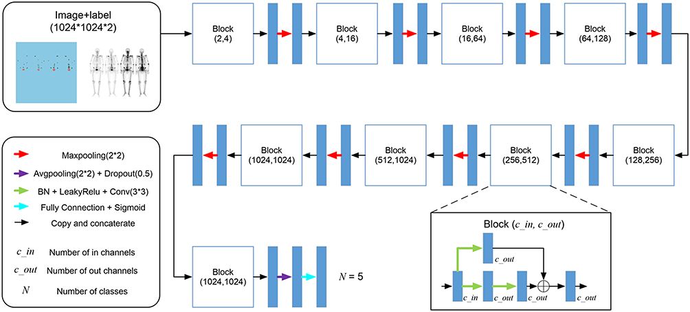Figure 4 Diagnostic report generation model structure.

Most of the lesions are concentrated in the spine, pelvis, scapula, ribs, and femur, so in this method, it was judged whether these five specific locations or other regions contain BMs. Cross-entropy loss was used as the loss function and trained with the SGD optimizer. Cross-entropy loss is often used for classification loss. The formula for cross-classification entropy loss is:

where are category tags, and is the probability that the model outputs 1.

Bone Scan Tumor Burden Index

Bone lesions are nonmeasurable lesions in the clinic since it is difficult to measure their size and range. Therefore, an objective evaluation method for bone tumor metastases is lacking. Here, we proposed using the bone scan tumor burden index (BSTBI), which can approximately calculate the overall tumor burden status of BMs. The formula is given as follows:

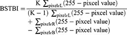
where L represents all pixels in the BM area, R represents all pixels on the bone scan image, B represents all pixels in the bladder area, K represents a scaling factor, K was 5 in this paper (when the value of K is 5, the BSBTI value is more approach to the normal distribution in our datasets.), and the pixel value represents the pixel value of the image. According to the formula, if the gray level is higher, the pixel value is smaller, and the tumor burden is larger, BSTBI∈[0, 1].

The research analyzed four frames of anterior-posterior bone scan image of every tumor patient with BMs who did not receive any treatment. The average BSBTI was calculated, and a Pearson correlation analysis with the corresponding blood ALP levels was performed to preliminarily verify whether BSTBI can reflect the tumor burden status of BMs in bone scan images and whether this parameter can be used as a quantitative index to evaluate the tumor burden of metastases.

Report Interpreter

The report interpreter translated the model’s predictions into popular language descriptions, including normal reports and abnormal reports (Table 2). If the classification model identified that the image data contained BMs, then the subsequent model would identify the location of the lesions, calculate the tumor burden, fill the results into the abnormal report template, and generate the final report, or the normal report template can be directly invoked.

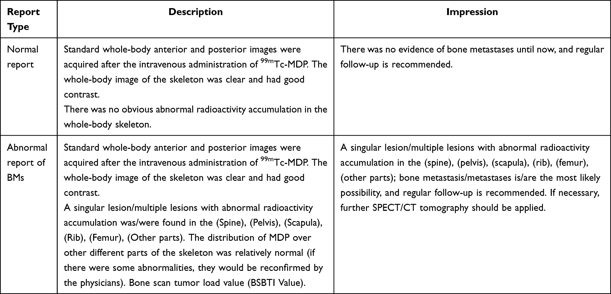Table 2 Report Template

Results

General Data

A total of 621 bone scan images were included in this research, from 280 patients with BMs and 341 patients with non-BMs (including 169 patients with no abnormal accumulation of MDP and 172 patients with MDP uptake of non-BMs mainly due to the degenerative diseases of joints or spine, trauma, operations, osteoporosis). According to the aforementioned image processing method, there were 498 cases in the training set, including 226 BMs and 272 non-BMs. A total of 123 cases were in the testing set, including 54 BMs and 69 non-BMs (Table 3).

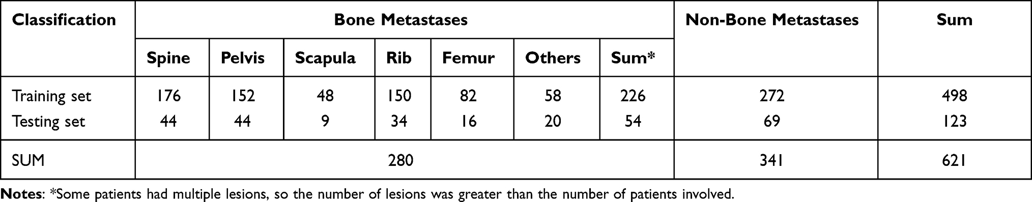Table 3 Bone Metastases and Normal Distribution in the Data Sets

Diagnostic Classification Model Results

The threshold for the classification model was set as 0.5. The performance of the diagnostic classification model on the whole-body image and its comparison with three nuclear medicine physicians (with less than 2 years, 5 years and 10 years related experience, respectively. All of them were blinded to the truth diagnosis during the process of comparison) are shown in Tables 4 and 5. The accuracy of physicians highly depended on their clinical experiences. The diagnostic classification model gained an accuracy of 88.62%, which showed no statistical difference with moderately and experienced physicians, but obviously outperformed the inexperienced. Meanwhile, excepting that the specificity of the model was lower than the experienced physician, the model still achieved good sensitivity and specificity. Additionally, area under the curve (AUC) of classification model for BMs and bladder were 0.9263, 0.9970, respectively, indicating the model of classification can effectively identify BMs and normal images, and distinguish BMs from the bladder (Figure 5A and B).

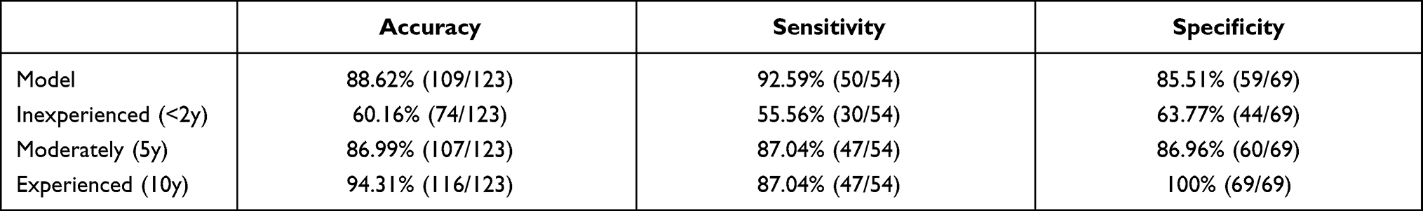Table 4 Performance of the Diagnostic Classification System on Whole-Body Images and Its Comparison with Three Nuclear Medicine Physicians (N=123)

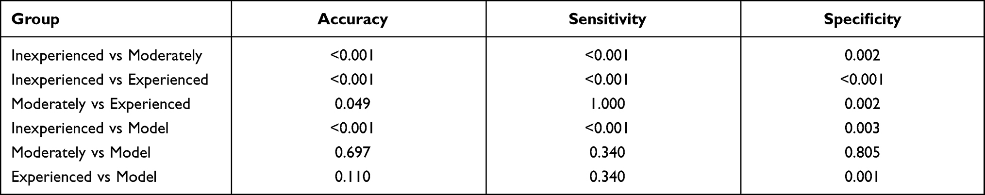Table 5 The Statistics Analysis About the Accuracy, Sensitivity, and Specificity Between the Diagnostic Classification Model and the Three Physicians (N=123)

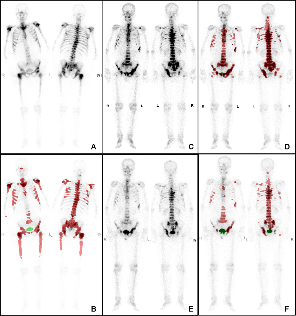Figure 5 The result of identification of bone metastases and the comparison of BSTBI before and after therapy. (A and B) A super bone image from a prostate tumor patient, the red area predicted by the model represents bone metastases; (C and D) A prostate tumor patient with extensive bone metastases, before therapy, the BSTBI values are 0.7531 (ANT), 0.8420 (POST); (E and F) The patient was treated with Zoledronic acid therapy. After 5 months, the BSTBI values are decreased to 0.5160 (ANT), 0.7940 (POST).

Metastasis Bone Tumor Segmentation Model Results

In the test set, the Dice coefficient of BMs and bladder of our method was 0.7387 and 0.9247. Compared with the manual labels, the results of this model prediction which makes analysis at the pixel level were even more accurate (Figure 2B and C). Contrastively, the Dice coefficient of BMs of the segmentation models based on the U-net and nnU-net directly were 0.6623 and 0.6819, respectively, which were lower than our method.

BSTBI Could Be Used as a Quantitative Analysis Indicator

BSTBI can reflect the tumor burden indicated on bone scintigram (Figure 6A), it changed as the BMs changed (Figure 5C–F). The peripheral blood ALP level of 50 patients with primary tumors diagnosed with BMs without any treatment were enrolled to verify the feasibility of BSBTI. The result of correlation analysis suggested that there was a positive correlation between BSBTI and blood ALP (r=0.72, P<0.05) (Figure 6B).

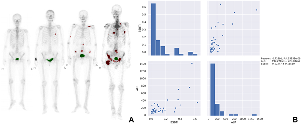Figure 6 BSTBI values. (A) From left to right, the values are 0, 0.0181, 0.1379, and 0.4432 (K=5). (B) Pearson correlation analysis between BSTBI and ALP (N=50). ALP, 197.23±228.88 (U/L); BSTBI, 0.12±0.16 (r=0.72, P<0.05).

Diagnostic Report Generation Model Results

The localization accuracy of BMs in the test set was 74.07% (40/54). The accuracies for specific locations were 95.45% (42/44) for the spine, 97.73% (43/44) for the pelvis, 44.44% (4/9) for the scapula, 91.18% (31/34) for the ribs, 81.25% (13/16) for the femur, and 90.00% (18/20) for other parts. There were 14 (25.93%, 14/54) cases of an incorrect location, including 5 in the scapular area, 3 in the femoral area, 2 in the rib area, 2 in other areas, 1 in the pelvis and 1 in the spinal area.

Of the 123 cases in the test set, 63 (59 correct and 4 false) cases were diagnosed as normal and normal reports were generated. Among the other 60 cases that were identified as BMs by the classification model, there were 37 cases with an accurate localization, 14 cases with a single incorrect localization prediction, and 9 cases with multiple incorrect localization predictions. Combined with the BSTBI, the final reports are shown in Figure 7. Hence, the accuracy of the report generation model was 78.05% ((59+37)/123), in contrast to 73.17% ((55+35)/123) based on Resnet34, which was lower than our method. Moreover, the time taken by the machine learning model in this study from raw data to report generation was 0.55 ± 0.07 s. Obviously, the model was very efficient.

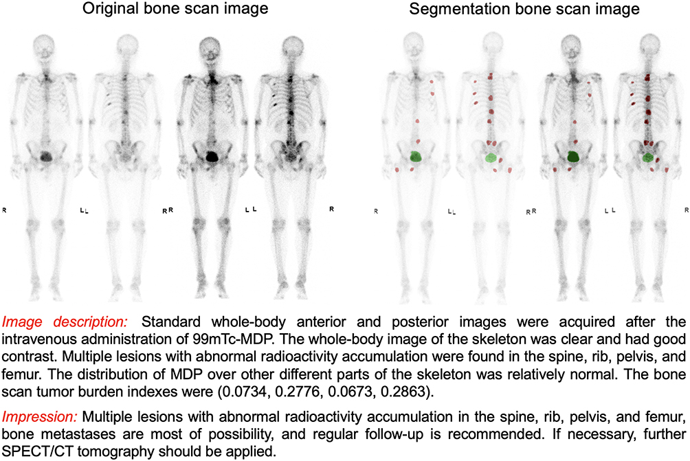Figure 7 Diagnostic report generation result. It includes the impression of the report and the BSTBI values.

Discussion

Mitsuru Koizumi⁷ et al used the CAD system BONENAVI version 2 to evaluate the accuracy of diagnosing BMs, adopting an artificial neural network (ANN) with a threshold of 0.5. The sensitivity and specificity were 85% and 82%, respectively. The highest accuracy was 72% for BMs of prostate cancer. Recently, CNNs, one of deep learning neural networks, are different from previous methods.^2–7 Instead of artificially designing features, they directly abstract features on the images, and are adopted in diagnosis of BMs on bone scan images, and have achieved good performance.^12–14 In our study, we adopted the classic ResNet34 learning method. The sensitivity, specificity and accuracy of diagnosing BMs were 92.59%, 85.51% and 88.62%, respectively, which were higher than the results of Mitsuru Koizumi’s study. They were similar to Yong’s,¹³ who used the attention-augmented deep neural networks to constructed an automated diagnosis model of BM, with the sensitivity of 92%, specificity of 86% and accuracy of 89%, but a little lower than Papandrianos’s because of different CNN frame. When compared to the nuclear medicine physician, our results suggested that the diagnostic classification model had good performance in identifying BMs which was comparable to physicians with more than 5 years’ work experience (the accuracy of moderately and experienced were 86.99% and 94.31%, P>0.05), and it could assist the physician in diagnosing, especially for those inexperienced physicians in primary hospitals. However, our work is not just focus on classification, but a series of models mainly on the quantitative analysis.

The previous work on bone scan segmentation mainly contains two directions: one is based on machine learning²⁶ and the other is based on deep learning methods. In machine learning, the code is not open source, and it is difficult to reproduce the code. In our study, deep learning was adopted, the Dice value of BMs between model identification and artificial identification was 0.7387. In addition, the BM segmentation model could segment the lesions at the pixel level. Compared with rough artificially delineated lesions, the segmentation model could delineate lesions more accurately because the model had relatively learned the range of pixel value of BMs, which was the essential of the quantitative analysis of BMs. We also directly applied the U-net and the state-of-the-art nnU-Net segmentation models based on the whole training set, on the contrary, the Dice of these two models were 0.6623 and 0.6819, both did not work out well. These results might be due to the whole training set containing many normal data which would inhibit the recognition of the model for the region of interest. That is, the model would recognize all the data as normal and would get a small loss; however, the actual results were not satisfied. We adopted the step-by-step method. Our segmentation model was also built on the U-net not with the whole training set but only the data containing BMs, this was consistent with our whole model frame, classification first and then segmentation. The performance of segmentation model was improved to 0.7387. Meanwhile, our model is more generalizable, except prostate cancer, we also included patients with lung cancer, breast cancer, gastrointestinal cancer.

At present, the assessment of tumor burden mostly depends on imaging, and BMs are always nonmeasurable. Even though professional physicians carefully evaluate the images, only rough evaluation can be given, such as lesion volume, number of lesions or an increase or decrease of MDP uptake. This assessment is largely affected by subjective factors, especially for patients with small changes, resulting in the quantitative analysis of BMs cannot be performed objectively and accurately. The reported quantitative assessment methods for BMs on bone scan images include the bone scan index (BSI),²⁷ positive area on a bone scan (PABS),²⁸ bone scan lesion area (BSLA),^4,29 bone scan lesion area intensity (BSLAI),²⁹ etc. The BSI and BSLA are the two most commonly used indicators for the quantitative analysis of tumor burden on bone images, but they were only applied to evaluate the efficacy of treatment for prostate cancer. Computing the BSLA involves automated image normalization, lesion segmentation, and summation of the total area of segmented lesions on anterior and posterior bone scans as a measure of tumor burden. The BSI sums the product of the estimated weight and the fractional involvement of each bone, which is determined visually or from lesion segmentation on the bone scan. The BSLA and BSI are based on ANNs, and both need to manually design features for classification, which is time-consuming and requires many manual labels.

In our study, we directly inputted the images and automatically extracted lesion features through a convolutional neural network (CNN), and we proposed BSTBI to calculate the overall tumor burden status of BMs. The BSTBI is the percentage of all BMs pixels among all pixels except the bladder in the bone scan image. It changes with the number of areas with MDP uptake, size of the area and degree of MDP uptake in the lesions. From the perspective of development and analytic validation, it is feasible for the BSTBI to reflect the tumor burden of BMs. In addition, 50 patients with tumors who were diagnosed with BMs for the first time and did not receive any treatment were enrolled, and our results suggested that peripheral blood ALP level was positively correlated with the corresponding BSTBI value (r=0.724, P<0.05). ALP is an enzyme that is widely distributed in the human liver, bones and so on and is excreted by the liver. This enzyme is very active in bone tissues, so increases or significant changes in ALP level can be regarded as one of the indicators for the diagnosis and prediction of skeletal system diseases, such as BMs,³⁰ when the bone is destroyed by tumors, and ALP is positively correlated with the classification of BMs. Herein, the factors affecting ALP level were excluded as much as possible. ALP level was positively correlated with BSTBI, preliminarily indicating that the BSTBI can reflect the tumor burden of BMs. During the learning process, our model can also identify and segment the bladder well, and can distinguish bladder from the metastases in pelvis. Therefore, when designing the BSTBI, our study excluded the pixels of the bladder area and used all pixels in the image except for those in the bladder as the background to calculate the percentage of all BMs. Compared with the BSI and BSLA, this calculation method has the advantage that it can eliminate influences due to tracer injection, scanning technology and image postprocessing and the bladder to the furthest extent and accurately reflect the tumor burden of BMs. Thus, we believe that the BSTBI could be used as one of the parameters to quantitatively evaluate the overall tumor burden of BMs on bone scan images and has optimistic clinical application prospects. In future work, the author will continue to evaluate the BSTBI in some new clinical trial data.

At the end of our study, the classification model, segmentation model, region positioning, and BSTBI were combined, and the analysis process was extended to a deep level of semantic segmentation and report generation, which enhanced the automation of the model and achieved a completely automatic analysis process from image input to final report generation. The accuracy of the whole process was 78.05%, and the entire analysis process greatly saved time, and it only took approximately 0.55 s on average. Moreover, with increases in workload, the efficiency of manual work will become increasingly lower, but AI will not be affected. Until now, no similar studies about report generation have been reported. Meanwhile, our report generation model was compared to the report generation model, which was based on Resnet34, our model performed better (78.05% Vs 73.17%). Among the 123 test sets, 63 cases finally generated normal reports. After being rejudged by a physician, 4 cases were wrong, mainly due to classification errors. The author thought that these cases were wrong for the following reasons: one case of sternal bone destruction and increased MDP uptake may have been misclassified due to the lack of training data of sternal metastases; and two cases of lumbosacral vertebrae bone destruction and mildly increased MDP uptake were judged as degenerative changes of the spine and generated a normal report finally. In our study, while training the model to identify BMs, we also trained the model to identify degenerative changes of the joints and spine. However, because of metastatic spinal cancer, especially small lesions with similar features, sometimes it was difficult to identify them from degenerative changes. Moreover, the training data of degenerative changes were insufficient, and good results have not been achieved, so this was not explained in this report. Finally, one patient had a small lesion located in the right sacrum, which was missed by the model. Sixty cases judged as BMs by the model eventually generated 37 accurate reports. The other 23 cases with reporting errors included 10 classification errors and 13 cases with incorrect regional locations. Among the 10 cases with classification errors, 7 cases with spinal degenerative diseases were misidentified as BMs, 2 cases were symmetric MDP accumulation of bilateral hip joints, and 1 case was in vitro pollution. The reasons for the incorrect regional location of lesions were, on the one hand, the insufficient data especially the data about the location of BMs on scapula (only 48 cases in the training set that led to the low location accuracy of scapula, as a result of pulling down the whole localization accuracy of BMs), which led to the limited generalizability of the model, and on the other hand, the incorrect segmentation results.

Although our research revealed the advantages and prospects of combining deep learning with bone scan images, the data and methods in this paper are still a proof of concept with some flaws. First, our data came from the same center. There may be some deviations from the distribution of actual data, which may cause the trained model to not perform well on all data. In the future, we will consider randomly selecting more data from different medical centers to validate the model in our study and to reduce the differences between different data centers. Second, because BMs are mainly located on the axial skeleton, there are little data about BMs located on other locations, such as the humerus and facial skull. The severe imbalance of the sample caused the model to be biased in locating the lesions. Third, the boundaries of BMs on bone scan images are very fuzzy. We cannot outline the precise boundary using existing labeling tools, which will also affect the deep learning model. We should seek for more precise labeling tools to improve the segmentation of bone lesions. Fourth, bone scintigraphy has high sensitivity but low specificity for skeletal lesions. During the process of training the model, we cannot ensure that every lesion labeled is a bone metastasis because it is impossible to scan every lesion with CT or other related examinations. This is a limitation of this examination method. Therefore, some normal images will be identified by the model as BMs, such as those of fractures and degenerative changes in the spine. This requires us to enlarge data about degenerative or other bone diseases to train the model, then the model could precisely identify them, in order to ease the work burden of the physician as far as possible. Finally, the bone scan flare phenomenon is one of the limiting factors in using the BSTBI as a quantitative indicator of tumor burden, especially in the evaluation of the therapeutic effect. The bone scan flare phenomenon is known to occur in many cancers, such as prostate cancer³¹ and breast cancer,³² and involves an increase in bone uptake during the healing process, usually 3–6 months after the commencement of effective therapy. This study did not assess serial bone scans after therapy. Theoretically, the BSTBI would have increased in such cases. Next, we will verify the practicalities of BSTBI in a prospective study about the therapeutic evaluation of BMs in prostate patients.

Conclusion

The model in our study preliminarily realized a fully automatic analysis process from raw data to report generation. The overall task was divided into three portions: diagnostic classification model, region segmentation model and diagnostic report generation model. Each model achieved good results. In addition, the author believes that the proposed BSTBI can be used as one of the indicators for the quantitative analysis of the tumor burden of BMs on bone scan images. Therefore, there is some clinical application prospect for this model to assist in the diagnosis and therapeutic evaluation of BMs. Our future work is oriented in optimizing our model with the newest neural networks, improving the generalizability of the model and verifying the value of BSTBI based on large sets of data.

References

1. Wang J, Li S. A brief report on the results of the national survey of nuclear medicine in 2020. Chin J Nucl Med Mol Imaging. 2020;40:747–749. doi:10.3760/cma.j.cn321828-20201109-00403
2. Chiu JS, Wang YF, Su YC, Wei LH, Liao JG, Li YC. Artificial neural network to predict skeletal metastasis in patients with prostate cancer. J Med Syst. 2009;33:91–100. doi:10.1007/s10916-008-9168-2
3. Sadik M, Hamadeh I, Nordblom P, et al. Computer-assisted interpretation of planar whole-body bone scans. J Nucl Med. 2008;49:1958–1965. doi:10.2967/jnumed.108.055061
4. Brown MS, Chu GH, Kim HJ, et al. Computer-aided quantitative bone scan assessment of prostate cancer treatment response. Nucl Med Commun. 2012;33:384–394. doi:10.1097/MNM.0b013e3283503ebf
5. Tokuda O, Harada Y, Ohishi Y, Matsunaga N, Edenbrandt L. Investigation of computer-aided diagnosis system for bone scans: a retrospective analysis in 406 patients. Ann Nucl Med. 2014;28:329–339. doi:10.1007/s12149-014-0819-8
6. Horikoshi H, Kikuchi A, Onoguchi M, Sjostrand K, Edenbrandt L. Computer-aided diagnosis system for bone scintigrams from Japanese patients: importance of training database. Ann Nucl Med. 2012;26:622–626. doi:10.1007/s12149-012-0620-5
7. Koizumi M, Wagatsuma K, Miyaji N, et al. Evaluation of a computer-assisted diagnosis system, BONENAVI version 2, for bone scintigraphy in cancer patients in a routine clinical setting. Ann Nucl Med. 2015;29:138–148. doi:10.1007/s12149-014-0921-y
8. Liao F, Liang M, Li Z, Hu X, Song S. Evaluate the malignancy of pulmonary nodules using the 3-D deep leaky noisy-OR network. IEEE Trans Neural Netw Learn Syst. 2019;30:3484–3495. doi:10.1109/tnnls.2019.2892409
9. Li X, Chen H, Qi X, Dou Q, Fu CW, Heng PA. H-denseunet: hybrid densely connected UNet for liver and tumor segmentation from CT volumes. IEEE Trans Med Imaging. 2018;37:2663–2674. doi:10.1109/tmi.2018.2845918
10. Chmelik J, Jakubicek R, Walek P, et al. Deep convolutional neural network-based segmentation and classification of difficult to define metastatic spinal lesions in 3D CT data. Med Image Anal. 2018;49:76–88. doi:10.1016/j.media.2018.07.008
11. Wang J, Fang Z, Lang N, Yuan H, Su MY, Baldi P. A multi-resolution approach for spinal metastasis detection using deep Siamese neural networks. Comput Biol Med. 2017;84:137–146. doi:10.1016/j.compbiomed.2017.03.024
12. Papandrianos N, Papageorgiou E, Anagnostis A, Papageorgiou K. Efficient bone metastasis diagnosis in bone scintigraphy using a fast convolutional neural network architecture. Diagnostics. 2020;10. doi:10.3390/diagnostics10080532
13. Pi Y, Zhao Z, Xiang Y, Li Y, Cai H, Yi Z. Automated diagnosis of bone metastasis based on multi-view bone scans using attention-augmented deep neural networks. Med Image Anal. 2020;65:101784. doi:10.1016/j.media.2020.101784
14. Han S, Oh JS, Lee JJ. Diagnostic performance of deep learning models for detecting bone metastasis on whole-body bone scan in prostate cancer. Eur J Nucl Med Mol Imaging. 2021. doi:10.1007/s00259-021-05481-2
15. World Health Organization. WHO Handbook for Reporting Results of Cancer Treatment. Geneva, Switzerland: World Health Organization; 1979:1–3.
16. Eisenhauer EA, Therasse P, Bogaerts J, et al. New response evaluation criteria in solid tumours: revised RECIST guideline (version 1.1). Eur J Cancer. 2009;45:228–247. doi:10.1016/j.ejca.2008.10.026
17. Forner A, Ayuso C, Varela M, et al. Evaluation of tumor response after locoregional therapies in hepatocellular carcinoma: are response evaluation criteria in solid tumors reliable? Cancer. 2009;115:616–623. doi:10.1002/cncr.24050
18. Engels B, Everaert H, Gevaert T, et al. Phase II study of helical tomotherapy for oligometastatic colorectal cancer. Ann Oncol. 2011;22:362–368. doi:10.1093/annonc/mdq385
19. Hoos A, Parmiani G, Hege K, et al. A clinical development paradigm for cancer vaccines and related biologics. J Immunother. 2007;30:1–15. doi:10.1097/01.cji.0000211341.88835.ae
20. Jung K, Lein M. Bone turnover markers in serum and urine as diagnostic, prognostic and monitoring biomarkers of bone metastasis. Biochim Biophys Acta. 2014;1846:425–438. doi:10.1016/j.bbcan.2014.09.001
21. Russell BC, Torralba A, Murphy KP, Freeman WT. LabelMe: a database and web-based tool for image annotation. Int J Comput Vis. 2008;77(1–3):157–173. doi:10.1007/s11263-007-0090-8
22. He K, Zhang X, Ren S, Jian S. Deep residual learning for image recognition.
23. Lin TY, Goyal P, Girshick R, He K, Dollár P. Focal loss for dense object detection. IEEE Trans Pattern Anal Mach Intell. 2017;4:2999–3007.
24. Ronneberger O, Fischer P, Brox T. U-Net: convolutional networks for biomedical image segmentation.
25. Isensee F, Jaeger PF, Kohl SAA, Petersen J, Maier-Hein KH. nnU-Net: a self-configuring method for deep learning-based biomedical image segmentation. Nat Methods. 2021;18:203–211. doi:10.1038/s41592-020-01008-z
26. Shan H, Jia X, Yan P, Li Y, Paganetti H, Wang G. Synergizing medical imaging and radiotherapy with deep learning. Mach Learn: Sci Technol. 2020;1(021001):25.
27. Imbriaco M, Larson SM, Yeung HW, Mawlawi OR, Scher HI. A new parameter for measuring metastatic bone involvement by prostate cancer: the bone scan index. Clin Cancer Res. 1998;4:1765–1772.
28. Noguchi M, Kikuchi H, Ishibashi M, Noda S. Percentage of the positive area of bone metastasis is an independent predictor of disease death in advanced prostate cancer. Br J Cancer. 2003;88:195–201. doi:10.1038/sj.bjc.6600715
29. Brown MS, Kim GHJ, Chu GH, et al. Quantitative bone scan lesion area as an early surrogate outcome measure indicative of overall survival in metastatic prostate cancer. J Med Imaging. 2018;5:011017. doi:10.1117/1.JMI.5.1.011017
30. Villemain A, Ribeiro Baptista B, Paillot N, et al. Predictive factors for skeletal-related events in lung cancer. Rev Mal Respir. 2020;37:111–116. doi:10.1016/j.rmr.2019.11.647
31. Pollen JJ, Witztum KF, Ashburn WL. The flare phenomenon on radionuclide bone scan in metastatic prostate cancer. AJR Am J Roentgenol. 1984;142:773–776. doi:10.2214/ajr.142.4.773
32. Koizumi M, Matsumoto S, Takahashi S, Yamashita T, Ogata E. Bone metabolic markers in the evaluation of bone scan flare phenomenon in BMs of breast cancer. Clin Nucl Med. 1999;24:15–20. doi:10.1097/00003072-199901000-00004
© 2022 The Author(s). This work is published and licensed by Dove Medical Press Limited. The full terms of this license are available at https://www.dovepress.com/terms.php and incorporate the Creative Commons Attribution - Non Commercial (unported, v3.0) License.
By accessing the work you hereby accept the Terms. Non-commercial uses of the work are permitted without any further permission from Dove Medical Press Limited, provided the work is properly attributed. For permission for commercial use of this work, please see paragraphs 4.2 and 5 of our Terms.