Control of confounding in the analysis phase – an overview for clinicians

Introduction

During the era of modern epidemiology, we have seen large health care databases and registries emerging, contemporary with technological achievements in computing, which has paved the way for a remarkable increase in observational studies. Confounding is the concept of comparability in observational studies, which hampers causal inference.^1–3 Confounding arises when a factor is associated with both the exposure (or treatment) and the outcome, eg, a disease or death, and is not part of the causal pathway from exposure to outcome. Hence, if we study the effect of hypertension on the risk of stroke, we cannot just compare hypertensive people against people without hypertension. The reason is that we may obtain spurious results, if we do not consider confounding factors, such as smoking, diabetes, alcohol intake and cardiovascular diseases, that are likely associated with both stroke and hypertension and are not on the causal pathway from hypertension to stroke. The effect on odds ratio (OR) estimates when controlling for these confounding factors was illustrated in a UK registry-based case–control study that among other things examined the association between stroke and untreated hypertension. The estimated OR for the association of interest increased from 2.9 to 3.5 after controlling for confounding.⁴ In this example, the magnitude of the association was underestimated, if not adjusting for confounding; however, confounding may also result in an overestimated effect, if not accounted for.

Once a potential confounding problem has been recognized, it may be dealt with in the design or the analysis phase.⁵ Standard methods used in the design phase involve randomization, restriction and matching. In randomized studies, patients are assigned randomly to exposure categories. Restriction means that only subjects with certain values for the potential confounders are selected (eg, certain sex and age groups), while matching involves the selection of the groups to be compared (exposed vs not exposed or cases vs controls) to be comparable with respect to the distribution of potential confounders. In registry-based observational studies, it is often insufficient to control for confounding only during the design phase of the study. Usually, we wish to account for several potential confounders, which may not be possible by either restriction or matching. For example, by restriction, we may end up with a very small cohort, limiting both the precision and the generalizability of the results of the analysis. Likewise, matching on several potential confounders may reduce the likelihood of finding comparison people for the people in the patient cohort. The two approaches are not mutually exclusive. In the UK example with stroke, diagnosed cases were matched with a group of controls with the same sex and age in the design phase, and then, a multivariable regression analysis was performed in which hypertension status and the potential confounders were incorporated in the analysis phase.⁴ In general, the control of confounding may involve design, analytical, and statistical concepts by which we can perform statistical adjustment, restructure data, remove certain observations or add comparison groups with certain characteristics (negative controls) to deal with confounding.^6,7

In the history of control of confounding during the analysis, we have advanced from simple stratification with only a few potential confounders collated from small manageable hospital files to complex modeling procedures, using high-dimensional propensity scores (HD-PSs) by which hundreds of potential confounders are extracted from large health care databases.

The questions are, however, what have we achieved by this change in the setting of epidemiological research? Did we lose important aspects in the analysis? Are novel analysis methods to control for confounding that have become widely used in recent years, such as PS methods, our main response to the confounding issue in large and complex data sets? In the present article, we attempted to answer these questions, focusing on a registry-based setting. We considered the topic from a hands-on perspective and tried to demystify the control for confounding during analysis by explaining and discussing the nature of the various methods and referring to examples from epidemiological studies.

From the simple to the complex – stratification, standardization and multivariable analysis

Stratification

Stratification is the starting point in many textbooks dealing with confounding in the analysis phase.^8,9 This is probably due to the simplicity of this method in which a data set is broken into a manageable number of subsets, called strata, corresponding to the levels of potential confounders (eg, age groups and sex). By comparing the overall cross-tabulation for the association between an exposure and an outcome (eg, a 2×2 table for alcohol consumption and myocardial infarction [MI]) with stratum-specific (eg, age group) cross-tabulations, it becomes evident whether a factor introduces confounding in the analysis. Thus, the stratum-specific associations (eg, measured as ORs) would deviate markedly from the overall association – refer the example in the study by Mannocci¹⁰ on the confounding effect of age on the association between alcohol consumption and MI. Age was a confounder since it was associated with alcohol consumption (alcohol consumption was most frequent among younger people) and with MI (MI was most common among the middle-aged people). The Mantel–Haenszel method¹¹ is commonly used to deal with confounding using stratification. The method summarizes the stratum-specific ORs by using a weighted average of them. This approach is generally attractive because of its applicability to a number of epidemiological measures such as OR, risk difference, risk ratio and incidence rate difference.^9,10

Stratification is an attractive method because of its simplicity; however, there are limitations to the number of factors that can be stratified, so that information can be extracted from the analysis.⁹ For example, 10 dichotomous factors would result in 2¹⁰=1,024 strata, and some strata may contain little or no data. In epidemiological research, we are expected to build on the current knowledge base and select numerous potential confounders, previously recognized, from the wealth of data that are potentially accessible from registries. Hence, when we attempt to control for confounding in the analysis, we will soon face the limitations of the stratification method regarding the number of potential confounders that are practically manageable. Stratification is therefore rarely used exclusively to control for confounding in studies that emanate from large health care databases. These days, it is used as an assisting tool in combination with other methods, and stratification may be used to identify effect measure modifications, ie, to demonstrate that the strength of the association between an exposure and an outcome depends on the value of another factor.

Standardization

Standardization provides another tool that can cope with confounding, although hampered by some of the same constraints as in stratification. Typically, disease or death rates are only standardized to age, and perhaps to sex and race, even in large registry-based studies. If more factors are considered, then separate analyses must be undertaken for specific subgroups. While stratification of confounders relies on information at the individual level in a study population, standardization involves the use of a reference population, obtained either from the data set or from an external source, such as data from a larger geographical scale. As an example, in a study based on the Korean Stroke Registry, age- and sex-standardized mortality ratios in stroke patients were calculated and compared across reasons for stroke, using the overall Korean population in 2003 as the reference population.¹²

There are two main approaches that handle confounding by standardization: direct and indirect standardization, resulting in adjusted rates and standardized ratios. Detailed descriptions of the two methods can be found in most introductory textbooks to epidemiology (eg, Kirkwood and Stern¹³). In general, direct standardization is recommended, because the consistency of comparisons is maintained, ie, a higher rate in one study population compared to another will be preserved also after direct standardization. That said, the very rate is dependent on characteristics of the selected reference population.¹⁴ When unstable rates are encountered across strata, eg, because of small numbers of patients in each stratum, indirect standardization should also be considered.¹³ In the example from Korea, indirect standardization was used to show that the standardized mortality ratios were higher among patients with unknown stroke etiology compared to patients with known etiology.¹²

Multivariable analysis

Multivariable regression analysis has been one of the most frequently used methods to control for confounding, and the use of this approach was particularly enhanced at a time when modeling tools were made readily available. With multivariable analysis, we get around the main limitation of stratification, as we obtain the possibility to adjust for many confounding variables in just one (assumed true) model.¹⁵ Thus, we can take advantage of more of the information available in a registry than when we use stratification. In epidemiology, multivariable analysis is typically seen in analyses in which ORs or hazard ratios (HRs) are estimated. Control for confounding by multivariable analysis relies on the same principles as stratification, ie, the factors of interest (eg, a risk factor, treatment or exposure) are investigated while the potential confounders are held constant. In multivariable analysis, this is done mathematically in one integrated process, however, under certain assumptions (Table S1) – here as an example of linearity for linear models. This assumption may be compromised when confounders with nonlinear effects are incorporated in a linear model as continuous variables. This leads to residual confounding (confounding remains despite controlled for in the analysis) unless other measures are taken (refer the study by Groenwold et al¹⁶ for examples and solutions).

Selection of potential confounders for multivariable models has been the subject of controversy.¹⁷ Confounder selection would typically rely on prior knowledge,¹⁸ possibly supported by a directed acyclic graph (DAG), that is a graphical depiction of the causal relationship between, eg, an exposure and an outcome together with potential confounders.⁶ In large study populations, the researcher would in many cases include all known measured potential confounders in the regression model. In a registry-based German study, 16 potential confounders were included in the analysis of the effect of treatment with tissue plasminogen activator (t-PA) on death (361 cases) among 6,269 ischemic stroke patients.¹⁹ There was indeed a remarkable drop in the OR between t-PA and death derived from a multivariable model, when adjusting for confounding (OR=1.93 compared to OR=3.35 in the crude, unadjusted analysis). Such generous inclusion of potential confounding factors in the multivariable model is unlikely to be a problem in this example, given that there are >20 outcome events (deaths) per factor included in the model.²⁰ Factors may be omitted from a multivariable model based on preliminary data-driven procedures, such as stepwise selection, change-in-estimate procedure, least absolute shrinkage and selection operator (LASSO),²¹ and model selection based on information criteria (eg, Akaike information criterion).²² It is important to recognize that data-driven variable selection is not related to the presence of confounding factors in the data set, and hence, there is a possibility that important confounders are discarded during such procedures.²³

Modifications of the multivariable model have been developed to better comply with the underlying assumptions or to avoid discarding variables. These include transformations of variables,¹⁶ shrinkage of parameter estimates²³ and random coefficient regression models.²⁴ Despite great flexibility when exploring associations between an exposure and an outcome while controlling for potential confounders, multivariable analysis does not directly identify whether a factor is a true confounder. Therefore, it is not clear whether residual confounding remains in the model.²⁵

PS – our main response to confounding?

In recent years, PS methods have become very popular as an approach to deal with confounding in observational studies. The idea of this method is to modify the study so that exposure or treatment groups that we want to compare become comparable without influence from confounding factors.²⁶ In a cohort study, we want to get rid of confounding due to factors measured at baseline – typically defined as the period before a drug use or treatment of interest. Already in the early history of modern epidemiology, stratification by a multivariate confounder score was recognized as an attractive approach.²⁷ This is comparable to the PS approach, as it combines information on a number of variables (potential confounders) into a single score for each individual person in a data set. This score is equivalent to the probability of an exposure, given the characteristics measured at baseline. There are four conceptual steps in the PS methods: 1) selection of potential confounders; 2) estimation of the PS; 3) use of the PS to make treatment/exposure groups comparable (covariate balance) and assessment of group comparability and 4) estimation of the association between treatment/exposure and outcome.

In the German study on stroke patients mentioned earlier, PS methods were applied in addition to a multivariable analysis.¹⁹ We will use the setting from this example to outline the principles of the underlying conceptual steps; further details on the methods can be found elsewhere.²⁶ In the example, we would start estimating the probability of the treatment with t-PA as a function of a number of baseline characteristics, such as the presence or absence of comorbidities (hypertension, diabetes, etc.), or person characteristics (age and sex).

Based on the PS values, we can now group individuals according to baseline characteristics – here, untreated patients and patients treated with t-PA. This can be done in several ways: matching, stratification, covariate adjustment and inverse probability (of treatment) weighting. There is an extensive literature on the different variants and the associated pros and cons^26,28–30 (Table S2). Different variants were applied in the example, and eventually, affected the results, ie, the ORs between t-PA and death ranged from 1.17 to 1.96,¹⁹ potentially leading to different conclusions, if considered separately. However, it is important to recognize that different variants may imply answering different research questions.^26,31 We discriminate between approaches that estimate the average effect of a treatment on the population (both treated and untreated individuals) and the average effect of treatment on those individuals who actually received the treatment. In the example with t-PA, the authors mentioned that differences in ORs between two weighting variants (inverse probability of treatment weighting and standardized mortality ratio weighting) likely derive from the fact that the two approaches are associated with different research questions,¹⁹ and this may also apply to other methods that are evaluated in the study.

An important step is to evaluate whether the treated and untreated groups are comparable. The evaluation cannot be offset by a goodness-of-fit (GOF) test, which is a general approach that provides a measure of how well a statistical model fits the data. However, this approach is usually meaningless in the large data sets that are typically extracted from health care databases. Furthermore, the GOF test may not tell the researcher whether important confounders were excluded from the analysis, neither in multivariable analysis nor in PS modeling.^26,32

The evaluation of the comparability of the groups of interest may involve measures of difference, testing or visual inspection of the PS distributions of the two groups – refer the study by Franklin et al³³ for a discussion under what circumstances the different approaches are considered useful. Imbalances between the two groups may necessitate that the estimation of the PS is reconsidered, meaning that the specification of the model that provides the PS is changed, another PS variant is applied or the data set is trimmed.³⁴ By trimming, a subset of data is extracted according to certain rules, and thus, the sample size is reduced, which in some cases may hamper the feasibility and interpretability of the results obtained by the PS method.

It may be difficult to balance the treatment groups in small samples or if the comparison groups are very different. Hence, the evaluation of balance represents an assurance that eventually we analyze comparable groups in the final analysis of the possible association between treatment and outcome, adjusted for (measured) confounding.

In the German study on stroke patients, there was an imbalance between the t-PA-treated and -untreated groups with a limited overlap of PSs among the two groups due to an exceptionally high proportion of untreated patients with low PS. The authors then restricted the study population to patients with a PS ≥0.05, which increased the comparability of the groups. In this setting, the results were also less sensitive to the choice of PS variant (matching and several regression adjustments) compared to the unrestricted approach.¹⁹

As with multivariable analysis, there is a possibility that unknown, unmeasured and residual confounding still exists after having applied the PS approach. In order to attempt to reduce this drawback, the HD-PS approach was developed.³⁵ The HD-PS method involves a series of conceptual steps,³⁵ which in essence can be condensed to: 1) specification of data source; 2) data-driven selection of potential confounders; 3) estimation of PS; 4) use of the PS to make groups of interest comparable and assessment of group comparability and 5) estimation of the association between treatment/exposure and outcome. Essentially, it is the selection process of confounders that makes the HD-PS method differ from the conventional PS methods. For the HD-PS method, large numbers of variables (often hundreds) are selected as potential confounders. As an example in a nationwide study in Taiwan, the HD-PS method was used to adjust for confounding.³⁶ Well-known prespecified confounders, eg, sex, age and comorbidities related to lifestyle, were incorporated in the analysis together with 500 additional potential confounders. The rationale is that some of these many variables are likely proxies for unmeasured confounders that are not available in the database or the researcher is not aware of. Accordingly, we may be able to deal with at least some of the unmeasured confounding that would not be considered in a conventional PS approach. However, there is little empirical evidence that the HD-PS method is better at controlling for unmeasured confounding than other methods, and adding several hundred empirically identified factors in an HD-PS setting may lead to comparable results to those that could also be obtained from a conventional PS setting.³⁷ In addition, despite examples of HD-PS analyses that provided estimates closer to the estimates obtained in randomized trials,³⁸ we cannot conclude that HD-PS is almost as good a tool as randomization.

Given the data greediness of the HD-PS method, its application is dependent on access to large databases, although it has also been demonstrated to be quite robust in a small sample setting (down to 50 exposed patients with an event).³⁸ It is important to be aware that variable selection in the HD-PS method is mainly data driven and in principle associated with the risk of omitting important confounders. That said, the benefit of including an excessive number of proxies for potential unmeasured confounders possibly outweighs the risk of discarding important confounders. In multivariable analysis and conventional PS analysis, we select the potential confounders to adjust for from a pool of variables that are thought to be possible true confounders. Despite measures taken during the variable selection process in the HD-PS method,³⁸ the generous inclusion of variables from databases may increase the likelihood that variables are not confounders but mediator, collider or instrumental variables – see definitions elsewhere.^39–41 This may lead to inappropriate adjustment that potentially provides spurious results. However, we are limited in our understanding of all the prospects and pitfalls of the HD-PS method, given its relatively recent origin, although exploration and refinements of the approach have already emerged.^42–44

Overall, we can conclude that the PS methods have several attractive characteristics in a registry-based setting. For example, PS seems more robust in situations with rare outcomes and common exposures than multivariable analysis.^45,46 However, even in a large sample setting, we may face the challenge of rare exposure (or treatment). The disease risk score (DRS) method is suitable to use under these circumstances, such as in the early market phase of a drug when reduction in confounder dimensions is likely important.^47–49 DRS is comparable to PS in so far that information from several variables is summarized in one single score.

The PS method cannot handle treatment defined as a continuous variable (eg, drug dosage), unless dosage is categorized, typically dichotomized into the presence or absence of treatment, associated with the risk of losing important information on the association between an exposure and baseline characteristics. DRS may again be an alternative to PS. That said, methods that are based on the inverse probability weighting (IPW) principle represent alternatives with a wide range of applications, because IPW may be generalized to a suite of different circumstances also including dichotomous and non-dichotomous exposure.⁵⁰ The German study of stroke comprised an additional analysis, which controlled for confounding by using the IPW principle.¹⁹ Time-varying exposure and thus time-dependent confounding may also be dealt with by methods based on IPW in the form of marginal structural models⁵¹ or structural nested models based on G-estimation.⁵²

What did we achieve and what have we lost?

It is important to stress that during selection of a method, there is no book of answers, and in many cases, simple methods may be equally valid as the complex methods. In addition to all the pros and cons of the different methods (Table S1), we may face an unusual setting or a data set with an odd structure that necessitates further consideration of the method that controls for confounding. Moreover, the specific research question that we wish to answer may determine the method selected to control for confounding (Table S2).

Both stratification and standardization represent ways of learning about the data, as we look at smaller units of the data set, and we may use these methods as preliminary analysis, before we use other methods such as multivariable analysis or PS methods to adjust for confounding. Thus, applying stratification or standardization assists in the understanding of the data at a detailed level, and we may become aware of associations in specific strata, otherwise overlooked. By the era of multivariable analysis, we may have lost some of this basic understanding of the data, because of the complexity introduced by incorporating numerous potential confounders in models. Nevertheless, we are still capable of understanding which factors substantially confound an association, and we can directly explore interactions between an exposure and other factors. After the introduction of the PS method, there has been an ongoing discussion on the advantages and disadvantages of this method as compared to multivariable analysis. Glynn et al⁵³ noticed that in the majority of studies that used both multivariable analysis and PS methods, there were no important differences in the results, and this was further confirmed by simulation studies. However, comparable results across different methods do not prove that proper adjustment of confounding was undertaken, eg, if the data quality of important confounders is poor or unmeasured confounding exists. The trend in analysis methods has dictated that we extract more and more information from databases, when attempting to account for confounding. This could potentially entail that we reduce unmeasured confounding just by chance, most notably in the HD-PS approach with the inclusion of hundreds of variables. However, there is no evidence that this method is superior to others, and even the HD-PS method would be flawed in the case that data on important confounders or their proxies are not available or if variables that are not true confounders are adjusted for.

Given the complexities of registries and data analysis, we wish to emphasize the critical importance of clinical input and of the interplay between clinicians and analysts (statisticians) during the statistical analysis. Clinicians may contribute with important scientific input regarding the initial list of potential confounders that should be considered and their availability in health care databases; if potential confounders are missing, which surrogate factors could then be used as a replacement? Clinicians may also provide essential information on technical elements of the statistical analysis such as how variables should be categorized, the functional forms of continuous variables (eg, linear vs nonlinear) and temporal aspects (eg, the relative importance of an event of MI 1 week vs 1 year ago). Finally, clinicians have expert knowledge on the nature of treatments and treatment allocation that can guide the analyst.

Requirements to the analysis in the future

In the future, it would be an achievement if we were better at identifying confounding factors. At present, the selection of potential confounders in models largely relies on assessments, eg, prior knowledge, DAGs and arbitrarily defined differences between crude and adjusted results, or on data-driven procedures decoupled from the confounder issue.^17,54 It would be desirable to minimize the uncertainty of a factor being a true confounder. In addition, confounder selection is commonly compromised by limited access to appropriate variables in registries.¹⁸ In this respect, it would also be desirable that information on lifestyle and severity of diseases were more widespread in registries, as these elements likely represent important confounding factors.^55–57 Software that extracts information from medical records and translates it into analyzable data has already been developed⁵⁸ and may likely assist in compiling data on lifestyle and severity of diseases. Furthermore, self-reporting systems, remote sensing technologies and automated data logging already exist to accumulate data on, eg, blood pressure, physical activity and heart rate. This could potentially develop into health care monitoring in a citizen science setting, just as this concept has evolved in other science disciplines.^59,60 The use of such less aggregated data than those present in the registries of today will surely improve our ability to incorporate relevant confounders or their proxies; however, most likely it necessitates novel and innovatory methods to deal with the confounder issue in the analysis phase. However, despite a remarkable development of methods that control for confounding and new data opportunities, it is unlikely that we will be able to account completely for confounding in the data collection process in a foreseeable future. Hence, confounding will remain a serious issue that needs to be acknowledged in the interpretation of our analyses.

Acknowledgments

A hearty thank you to the editor and three anonymous reviewers for very useful comments, Lars Pedersen and Jan Vandenbroucke for stimulating discussions, Thomas B. Rasmussen for input to the PS methods and Kasper Adelborg and Troels Munch for their great hands-on knowledge on data collection in hospitals. This article was funded by the Program for Clinical Research Infrastructure (PROCRIN) established by the Lundbeck Foundation and the Novo Nordisk Foundation and administered by the Danish Regions.

Disclosure

The authors report no conflicts of interest in this work.

References

1.		Vandenbroucke JP. The history of confounding. Soz Praventiv Med. 2002;47(4):216–224.
2.		Morabia A. History of the modern epidemiological concept of confounding. J Epidemiol Commun H. 2011;65(4):297–300.
3.		Greenland S, Robins JM. Identifiability, exchangeability, and epidemiological confounding. Int J Epidemiol. 1986;15(3):413–419.
4.		Du X, Cruickshank K, McNamee R, et al. Case-control study of stroke and the quality of hypertension control in North West England. BMJ. 1997;314(7076):272–276.
5.		Greenland S, Morgenstern H. Confounding in health research. Annu Rev Publ Health. 2001;22:189–212.
6.		Greenland S, Pearl J, Robins JM. Causal diagrams for epidemiologic research. Epidemiology. 1999;10(1):37–48.
7.		Schneeweiss S, Suissa S. Advanced approaches to controlling confounding in pharmacoepidemiologic studies. In: Strom BL, Kimmel SE, Hennesy S, editors. Textbook of Pharmacoepidemiology. 2nd ed. UK: John Wiley & Sons Ltd; 2013:324–336.
8.		Kestenbaum B. Epidemiology and Biostatistics – An Introduction to Clinical Research. New York: Springer; 2009.
9.		Rothman K. Epidemiology – An Introduction. UK: Oxford University Press; 2002.
10.		Mannocci A. The Mantel-Haenszel procedure. 50 years of the statistical method for confounders control. Ital J Public Health. 2009;6(4):338–340.
11.		Mantel N, Haenszel W. Statistical aspects of the analysis of data from retrospective studies of disease. J Natl Cancer I. 1959;22(4):719–748.
12.		Nam HS, Kim HC, Kim YD, et al. Long-term mortality in patients with stroke of undetermined etiology. Stroke. 2012;43(11):2948–2956.
13.		Kirkwood BR, Sterne JAC. Medical Statistics. UK: Blackwell; 2003.
14.		Choi BCK, de Guia NA, Walsh P. Look before you leap: stratify before you standardize. Am J Epidemiol. 1999;149(12):1087–1096.
15.		Vandenbroucke JP. Should we abandon statistical modeling altogether. Am J Epidemiol. 1987;126(1):10–13.
16.		Groenwold RHH, Klungel OH, Altman DG, et al. Adjustment for continuous confounders: an example of how to prevent residual confounding. CMAJ. 2013;185(5):401–406.
17.		Walter S, Tiemeier H. Variable selection: current practice in epidemiological studies. Eur J Epidemiol. 2009;24(12):733–736.
18.		Brookhart MA, Sturmer T, Glynn RJ, Rassen J, Schneeweiss S. Confounding control in healthcare database research: challenges and potential approaches. Med Care. 2010;48(6 suppl):S114–S120.
19.		Kurth T, Walker AM, Glynn RJ, et al. Results of multivariable logistic regression, propensity matching, propensity adjustment, and propensity-based weighting under conditions of nonuniform effect. Am J Epidemiol. 2006;163(3):262–270.
20.		van Smeden M, de Groot JAH, Moons KGM, et al. No rationale for 1 variable per 10 events criterion for binary logistic regression analysis. BMC Med Res Methodol. 2016;16(1):163.
21.		Tibshirani R. The lasso method for variable selection in the Cox model. Stat Med. 1997;16(4):385–395.
22.		Akaike H. New look at statistical-model identification. IEEE T Automat Contr. 1974;Ac19(6):716–723.
23.		Greenland S. Invited commentary: variable selection versus shrinkage in the control of multiple confounders. Am J Epidemiol. 2008;167(5):523–529.
24.		Greenland S. When should epidemiologic regressions use random coefficients? Biometrics. 2000;56(3):915–921.
25.		McNamee R. Regression modelling and other methods to control confounding. Occup Environ Med. 2005;62(7):500–506.
26.		Austin PC. An introduction to propensity score methods for reducing the effects of confounding in observational studies. Multivar Behav Res. 2011;46(3):399–424.
27.		Miettinen OS. Stratification by a multivariate confounder score. Am J Epidemiol. 1976;104(6):609–620.
28.		Pirracchio R, Resche-Rigon M, Chevret S. Evaluation of the propensity score methods for estimating marginal odds ratios in case of small sample size. Bmc Med Res Methodol. 2012;12:70.
29.		Austin PC, Mamdani MM. A comparison of propensity score methods: a case-study estimating the effectiveness of post-AMI statin use. Stat Med. 2006;25(12):2084–2106.
30.		D’Agostino RB. Propensity scores in cardiovascular research. Circulation. 2007;115(17):2340–2343.
31.		Williamson E, Morley R, Lucas A, Carpenter J. Propensity scores: from naive enthusiasm to intuitive understanding. Stat Methods Med Res. 2012;21(3):273–293.
32.		Weitzen S, Lapane KL, Toledano AY, Hume AL, Mor V. Weaknesses of goodness-of-fit tests for evaluating propensity score models: the case of the omitted confounder. Pharmacoepidemiol Drug Saf. 2005;14(4):227–238.
33.		Franklin JM, Rassen JA, Ackermann D, Bartels DB, Schneeweiss S. Metrics for covariate balance in cohort studies of causal effects. Stat Med. 2014;33(10):1685–1699.
34.		Sturmer T, Rothman KJ, Avorn J, Glynn RJ. Treatment effects in the presence of unmeasured confounding: dealing with observations in the tails of the propensity score distribution – a simulation study. Am J Epidemiol. 2010;172(7):843–854.
35.		Schneeweiss S, Rassen JA, Glynn RJ, Avorn J, Mogun H, Brookhart MA. High-dimensional propensity score adjustment in studies of treatment effects using health care claims data. Epidemiology. 2009;20(4):512–522.
36.		Hung T-Y, Lee Y-K, Huang M-Y, Hsu C-Y, Su Y-C. Increased risk of ischemic stroke in patients with burn injury: a nationwide cohort study in Taiwan. Scand J Trauma Resusc Emerg Med. 2016;24(1):44.
37.		Toh S, Rodriguez LAG, Hernan MA. Confounding adjustment via a semi-automated high-dimensional propensity score algorithm: an application to electronic medical records. Pharmacoepidem Dr S. 2011;20(8):849–857.
38.		Rassen JA, Glynn RJ, Brookhart MA, Schneeweiss S. Covariate selection in high-dimensional propensity score analyses of treatment effects in small samples. Am J Epidemiol. 2011;173(12):1404–1413.
39.		Hernan MA, Hernandez-Diaz S, Werler MM, Mitchell AA. Causal knowledge as a prerequisite for confounding evaluation: an application to birth defects epidemiology. Am J Epidemiol. 2002;155(2):176–184.
40.		VanderWeele TJ, Vansteelandt S. Conceptual issues concerning mediation, interventions and composition. Stat Interface. 2009;2(4):457–468.
41.		Greenland S. An introduction to instrumental variables for epidemiologists. Int J Epidemiol. 2000;29(6):1102.
42.		Schneeweiss S, Eddings W, Glyn RJ, Franklin JM. Improving empirical variable selection in propensity-score models with high-dimensional covariate space using healthcare databases. Pharmacoepidem Dr S. 2014;23:11–11.
43.		Le HV, Poole C, Brookhart AM, Schoenbach VJ, Beach KJ, Sturmer T. Effects of aggregation of medical codes on the performance of the high-dimensional propensity score (hd-PS) algorithm. Pharmacoepidem Dr S. 2013;22:181–181.
44.		Franklin JM, Eddings W, Glynn RJ, Schneeweiss S. Regularized regression versus the high-dimensional propensity score for confounding adjustment in secondary database analyses. Am J Epidemiol. 2015;182(7):651–659.
45.		Winkelmayer WC, Kurth T. Propensity scores: help or hype? Nephrol Dial Transplant. 2004;19(7):1671–1673.
46.		Cepeda MS, Boston R, Farrar JT, Strom BL. Comparison of logistic regression versus propensity score when the number of events is low and there are multiple confounders. Am J Epidemiol. 2003;158(3):280–287.
47.		Glynn RJ, Gagne JJ, Schneeweiss S. Role of disease risk scores in comparative effectiveness research with emerging therapies. Pharmacoepidem Dr S. 2012;21:138–147.
48.		Arbogast PG, Ray WA. Use of disease risk scores in pharmacoepidemiologic studies. Stat Methods Med Res. 2009;18(1):67–80.
49.		Schmidt AF, Klungel OH, Groenwold RHH, Consortium G. Adjusting for confounding in early postlaunch settings going beyond logistic regression models. Epidemiology. 2016;27(1):133–142.
50.		Hernán M, Robins JM. Estimating causal effects from epidemiological data. J Epidemiol Community Health. 2006;60:578–586.
51.		Robins JM, Hernan MA, Brumback B. Marginal structural models and causal inference in epidemiology. Epidemiology. 2000;11(5):550–560.
52.		Robins J. A new approach to causal inference in mortality studies with a sustained exposure period – application to control of the healthy worker survivor effect. Math Modelling. 1986;7(9–12):1393–1512.
53.		Glynn RJ, Schneeweiss S, Sturmer T. Indications for propensity scores and review of their use in pharmacoepidemiology. Basic Clin Pharmacol. 2006;98(3):253–259.
54.		Hoffmann K, Pischon T, Schulz M, Schulze MB, Ray J, Boeing H. A statistical test for the equality of differently adjusted incidence rate ratios. Am J Epidemiol. 2008;167(5):517–522.
55.		Jiao L, Silverman DT, Schairer C, et al. Alcohol use and risk of pancreatic cancer. Am J Epidemiol. 2009;169(9):1043–1051.
56.		Di Milia L, Vandelanotte C, Duncan MJ. The association between short sleep and obesity after controlling for demographic, lifestyle, work and health related factors. Sleep Med. 2013;14(4):319–323.
57.		Weinhandl, Peng Y, Gilbertson DT, Bradbury BD, Collins AJ. Hemoglobin variability and mortality: confounding by disease severity. Am J Kidney Dis. 2011;57(2):255–265.
58.		Hinchcliff M, Just E, Podlusky S, Varga J, Chang RW, Kibbe WA. Text data extraction for a prospective, research-focused data mart: implementation and validation. Bmc Med Inform Decis Mak. 2012;12:106.
59.		Resnik DB, Elliott KC, Miller AK. A framework for addressing ethical issues in citizen science. Environ Sci Policy. 2015;54:475–481.
60.		Kelling S, Fink D, La Sorte FA, Johnston A, Bruns NE, Hochachka WM. Taking a ‘Big Data’ approach to data quality in a citizen science project. Ambio. 2015;44:S601–S611.

Supplementary materials

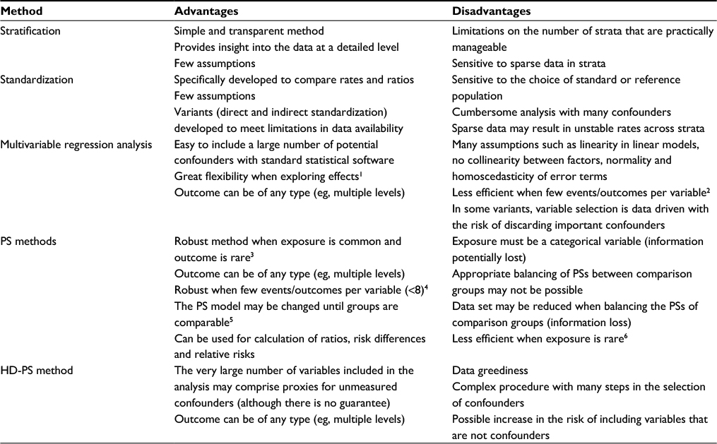Table S1 Summary of the pros and cons of five methods used to control confounding in observational studies Abbreviations: PS, propensity score; HD-PS, high-dimensional propensity score.

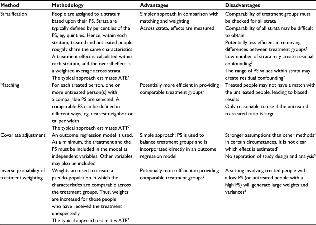Table S2 Summary of the methodological pros and cons of four different types of PS methods Abbreviations: PS, propensity score; ATE, average treatment effect for the population (both treated and untreated people); ATT, average treatment effect among treated people.

References

1.		McNamee R. Regression modelling and other methods to control confounding. Occup Environ Med. 2005;62(7):500–506.
2.		Peduzzi P, Concato J, Kemper E, Holford TR, Feinstein AR. A simulation study of the number of events per variable in logistic regression analysis. J Clin Epidemiol. 1996;49(12):1373–1379.
3.		Arbogast PG, Ray WA. Use of disease risk scores in pharmacoepidemiologic studies. Stat Methods Med Res. 2009;18(1):67–80.
4.		Cepeda MS, Boston R, Farrar JT, Strom BL. Comparison of logistic regression versus propensity score when the number of events is low and there are multiple confounders. Am J Epidemiol. 2003;158(3):280–287.
5.		Austin PC. An introduction to propensity score methods for reducing the effects of confounding in observational studies. Multivar Behav Res. 2011;46(3):399–424.
6.		Glynn RJ, Gagne JJ, Schneeweiss S. Role of disease risk scores in comparative effectiveness research with emerging therapies. Pharmacoepidem Dr S. 2012;21:138–147.
7.		Williamson E, Morley R, Lucas A, Carpenter J. Propensity scores: from naive enthusiasm to intuitive understanding. Stat Methods Med Res. 2012;21(3):273–293.
8.		Robins JM, Hernan MA, Brumback B. Marginal structural models and causal inference in epidemiology. Epidemiology. 2000;11(5):550–560.