Big data in sleep medicine: prospects and pitfalls in phenotyping

Introduction

Polysomnography (PSG) offers a wealth of physiological information, informing clinical decision-making and clinical research. Large sleep-related datasets are increasingly available for public analysis. For example, the National Sleep Research Resource (NSRR),¹ PhysioNet (www.physionet.com), the Montreal Archive of Sleep Studies (MASS),² and even consumer-facing efforts are underway.³ As “big data” analysis efforts gain momentum, it is increasingly important to understand not only the potential benefits but also the potential pitfalls of PSG phenotyping. In an era when in-laboratory PSG is increasingly restricted, enhancing signal processing and big data analytics could justify resource allocation to inform individual- and population-level insights.

The goals of sleep phenotyping span basic and clinical investigations as well as genotype–phenotype associations, especially as academic centers are increasingly banking bio-samples. Advanced knowledge about normal and pathologic sleep physiology might be derived from studying the relationship between sleep-disordered breathing events and heart rate variability, or about how electromyography (EMG) dynamics in rapid eye movement (REM) sleep vary depending on the presence of different medications and disease states. Big data insights might link indices of fragmentation to comorbidities or predict response to treatment of obstructive sleep apnea (OSA).

The opportunity for advanced analysis and phenotyping from the rich data obtained in routine clinical practice cannot be overstated. However, the allure of big data should not distract from the potential risks associated with even basic statistics and inferential efforts. Numerous cautionary statistical articles^4–12 and even entire monographs^13–15 have been published in recent decades highlighting the existence (and persistence) of common statistical misconceptions and pitfalls in basic and clinical research contexts. Large datasets do not mitigate these risks and in fact may present further challenges. We explore various kinds of PSG data in this framework, including insights and pitfalls from the existing literature, and through empirical analysis of a large dataset of diagnostic PSGs from our center. With the growing capacity for large-scale analytics, recognizing the strengths and limitations of phenotyping will help maximize the utility of large database resources.

Methods

The Partners Institutional Review Board (IRB) approved retrospective analysis of our database without requiring additional consent for use of the clinically acquired data (IRB number: 2009P000758). We selected diagnostic PSGs from adults in our database from 2011 to 2015, yielding n=1835 studies in our dataset. We did not have any exclusion criteria.

PSG was performed and scored according to the American Academy of Sleep Medicine (AASM) practice standards. Channels included six electroencephalogram leads, bilateral electrooculogram, submentalis EMG, nasal thermistor, oronasal airflow, snore vibration sensor, single-lead electrocardiogram (ECG), chest and abdomen effort belts, pulse oximetry, and bilateral anterior tibialis EMG.

From presleep questionnaires, we analyzed self-reported symptoms associated with sleep apnea, insomnia, restless legs, and narcolepsy. OSA symptoms included checkboxes spanning symptoms of sleep apnea, such as snoring, gasping, and witnessed apnea. Insomnia symptoms included checkboxes for difficulty regarding sleep onset (30–60 minutes or >60 minutes of sleep-onset latency), sleep maintenance (>3 awakenings per night), and insomnia as the reason for the PSG. Although at the time our intake form included “waking earlier than desired”, we have found clinically that, for this question, many false positives were occurring (e.g., work requiring early waking, as not desirable), and thus we did not include in our current analysis. Restless leg syndrome (RLS) symptoms included checkboxes for legs feeling uncomfortable, feeling better with movement, and feeling worse at night. Narcolepsy symptoms included checkboxes for perisleep hallucinations, sleep paralysis, and cataplexy. The intake form was designed to provide basic language symptom inventories, but it has not been independently validated against clinical diagnosis of sleep physician evaluation. We did not include standardized questionnaires for each of the many subcomponents, to strike a balance between information that assists providers in interpreting PSG data and the burden on patients. As the majority (>70%) of patients undergoing PSG in our center are direct referrals (have not seen a sleep specialist in our division before the PSG), we did not have clinical interview-based validation of the symptom reporting.

Statistical analyses were performed using GraphPad Prism 6 software (GraphPad Software Inc., La Jolla, CA, USA).

Results and discussion

In the following sections, we combine the analysis of simulated data with the analysis of a large sample (n=1835) of diagnostic PSG data from our center to illustrate important considerations in analyzing big data in sleep medicine. We can consider four basic categories of information that support clinical phenotyping derived from PSG databases (Figure 1). In each category, methods of cleaning and analysis are implemented, which we discuss in the following sections. Inferential analysis and insights can also be obtained by combining information across categories. For example, correlation and regression analysis can be performed on variables within or between categories, as can more complex predictive analytics be performed using methods of supervised machine learning. Unsupervised learning, also known as clustering, can be applied as well for discovery of novel phenotypes.

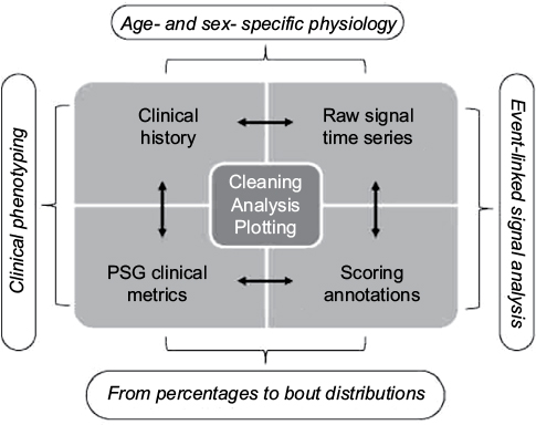Figure 1 Analysis hierarchy. Notes: Categories of sleep data obtained from or associated with clinical PSG recordings. Each requires core processes of cleaning, analysis, and plotting. Combining information between categories can provide further insights, such as linking scored events (e.g., PLMS) and physiology (ECG changes), or using stage annotations to calculate transition frequencies as an adjunct to stage percentage. Abbreviations: PLMS, periodic limb movements of sleep; PSG, polysomnography; ECG, electrocardiogram.

Standard PSG metrics and data types

The standard metrics in most clinical PSG reports are readily accessible in sleep databases without requiring off-line extra processing. These include basic demographics and summary statistics of PSG scoring, such as stage percentages, total sleep time (TST), efficiency, and apnea–hypopnea index (AHI). The importance of standardization in human scoring and basic metrics has been emphasized, especially for multicenter trials and data repositories involving PSG.¹⁶ Clinical metrics should be assessed in several steps to prepare for large-scale analytics.

PSG scoring annotations

PSG annotations include technician-scored labels for sleep–wake stage and various events (arousals, limb movements, breathing events) often with time stamps. These data can be exported for off-line processing and/or combining with other sources of clinical information. Aligning these files with exported time series data allows stage- or event-specific analysis of physiological signals.

Event label errors include errors of omission and of commission, and they are best assessed by manual rescoring. Some scoring errors may have indirect effects, such as failure to score an epoch of wake that interrupted a block of REM, which will have the dual effect of missing an awakening and resulting in a larger REM bout duration measurement.

Annotation data are also commonly used for inter-rater reliability analysis, or in groupwise comparisons of technician- or center-level differences in scoring. Because inter-rater reliability for various scoring tasks tends to be in the 80%–85% range,¹⁷ this sets a theoretical ceiling for performance of automated algorithms.

PSG time series data

Each channel of a standard PSG is a time series, to which a number of signal processing techniques can be applied to extract information. Initial preprocessing can involve detection and removal of periods with prominent muscle artifact, or removal of ECG signal contaminating electroencephalography (EEG) channels, or de-trending if slow drift is present.

Spectral analysis of the EEG is commonly performed using the fast Fourier transform (FFT) algorithm, which is applied using a moving window to produce an image of spectral characteristics as they change over time. However, the FFT alone provides noisy estimates of the underlying spectral characteristics of the data; thus, it is common to apply spectral and temporal smoothing to improve the estimates. The multi-taper spectral analysis method optimizes the trade-off between retaining fine details (spectral and temporal resolution) while still reducing noise (variance reduction).¹⁸ EEG time series analysis is common in research settings but has not enjoyed similar clinical applications in routine practice, although some clinical acquisition software includes basic frequency analysis options.

The ECG time series has been the subject of extensive analysis of heart rate variability,¹⁹ as well as point-process modeling variants.²⁰ Another method of ECG analysis, known as cardiopulmonary coupling (CPC), has been suggested to provide an important window into sleep quality beyond that observed in EEG-defined states. Whereas stable non-REM (NREM) sleep is characterized by stable breathing and “high-frequency” coupling (HFC) at the respiratory frequency, processes that disrupt sleep tend to increase low-frequency coupling (LFC). Of particular interest is that treatment-emergent central apnea (and clinical failure of continuous positive airway pressure [CPAP]) was predicted by the degree of narrow band LFC.²¹ Whereas obstructive apnea is characterized by the broadband LFC phenotype, chemoreceptor-driven sleep apnea (e.g., central apnea) is associated with narrow band coupling.

Self-reported clinical information

Patients undergoing in-laboratory PSG are often asked to self-report symptoms, medical problems, and medications in the questionnaire form. Our center uses a custom form as a basic symptom and history screening tool, which includes the Epworth Sleepiness Scale (ESS), as well as checkboxes and boxes for free-text responses. When self-reporting methods are used, the data require manual or semiautomated review and cleaning before analysis is possible. If medications are listed as free text, spelling errors or nonstandard terminology (e.g., sleeping pill) requires reconciliation. Internal inconsistencies require attention, such as listing multiple antihypertensive medications but not listing hypertension in the medical history. We found ~75% concordance between listing hypertension from a checkbox selection of medical problems and listing of antihypertensive agents (data not shown). Such a discrepancy could be a simple omission or could be that the patient is on treatment and thus no longer feels they have the disorder.

Combining information categories to inform phenotyping

Using simple combinations of existing metrics, or more involved extractions from the clinical scoring (annotation files), additional data for phenotyping can be generated beyond that which may be available in the acquisition software system. For example, event-related signal analysis, manual scoring annotations, and temporally associated time series data can be combined to explore phenotypes. Several examples of event-specific metrics have been reported, with potential clinical relevance. Chervin et al^22,23 analyzed respiratory event-linked EEG changes to sub-phenotype OSA patients and found a stronger relation with sleepiness by this advanced analysis compared to the usual AHI value. EEG analysis of alpha power and spindle activity has been used to predict arousal response to auditory stimulation delivered during sleep,^24,25 reflecting possible biomarkers of sleep fragility. Additional work investigating arousals and autonomic features highlights opportunities to stratify episodic physiological events during sleep that are not currently distinguished in routine scoring.^26–32

Database-driven sleep phenotyping

Symptom heterogeneity

We used a convenience sample of n=1835 individuals who underwent diagnostic PSG in our laboratory. In this dataset, symptom combinations were common. Figure 2 illustrates the overlap between self-reported OSA symptoms, insomnia symptoms, and leg-related symptoms in the cohort. The majority of individuals reported more than one of these categories, with less than one-third reporting from only one category. Within the group reporting OSA symptoms, isolated snoring was present in over half, with nearly as many reporting a combination of snoring and either gasping arousals or witnessed apneas (Figure S1). Among those with insomnia symptoms, difficulties with sleep maintenance was the most common isolated symptom, while about half reported more than one insomnia symptom or checked “insomnia” from a list of reasons for the study, along with at least one insomnia symptom (Figure S1). In rare cases, insomnia was listed as the reason for study by the patient, but no insomnia symptoms were checked. Among those with leg symptoms, about one-quarter reported all three symptoms consistent with RLS (uncomfortable sensation while awake, worse at night, better with movement; Figure S2). Narcolepsy symptoms were the least common. The isolated reporting of only one of the three cardinal REM-related phenomena was more common than combinations of any two or all three (Figure S2).

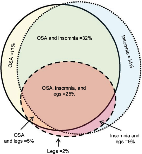Figure 2 Symptom overlap reported by adults undergoing diagnostic PSG. Notes: OSA symptoms and insomnia symptoms commonly coexisted (solid with yellow fill, and dotted with blue fill, respectively). Leg symptoms (either RLS or PLMS) were also commonly present (dashed circle with red fill). The area of the shapes approximate the n-value (sample size) for each category: OSA only =210; insomnia only =253; legs only =32; OSA and insomnia =584; legs and insomnia =166; OSA and legs =89; OSA and legs and insomnia =454. Abbreviations: OSA, obstructive sleep apnea; PLMS, periodic limb movements of sleep; PSG, polysomnography; RLS, restless leg syndrome.

Sleep–wake architecture and fragmentation

Sleep–wake stages are most commonly reported as the number of minutes, and relative percentage of wake, REM, and N1–3. Stage percentage during PSG may be noted in clinical interpretations, and there are normative data available across the lifetime.³³ In some settings, such coarse descriptive metrics may be useful. For example, when commenting on the presence or severity of sleep apnea, one might consider the potential for underestimation if the night happened to contain little or no REM, as OSA is often more pronounced in REM sleep (i.e., REM dominant). A relative increase in N3 percentage may suggest rebound sleep after recent deprivation. Certain medications may alter stage composition (e.g., commonly by reducing REM or N3).^34,35 Thus, stage percentage might combine with other categories of information, such as the clinical history, rather than provide a basis for actionable clinical recommendations in isolation.

A somewhat more granular approach to sleep architecture is to quantify sleep fragmentation, for example, via sleep efficiency, or by increased time spent in N1 (often because of frequent arousals), or reduced time spent in REM or N3 that may indirectly occur.^36,37 We can consider the use of sleep efficiency to describe two patients with very different hypnograms, but similar efficiency values. Because efficiency does not distinguish between different patterns of wake after sleep onset (WASO), it runs the risk of lumping together quite different patterns of fragmentation.³⁸ Figure 3 shows two PSGs with similar sleep efficiency, but which differ by fivefold in terms of the number of transitions to the wake state. In fact, the PSG with greater frequency of wake transitions (Figure 3B) actually has a slightly higher efficiency than the PSG with fewer but longer wake bouts (Figure 3A; 82% versus 78%, respectively). The reasons behind these patterns, the potential clinical impact, and therapeutic considerations may be quite distinct. Figure 3C–G shows the distribution of several metrics in a cohort of n=100 individuals with sleep efficiency values of 79.5%–80.5%. These broadly distributed values are a reminder that a sleep efficiency of “80%” can not only be achieved with distinct patterns of wake but can also be associated with diverse patterns of other potential contributors to (or markers of) fragmentation.

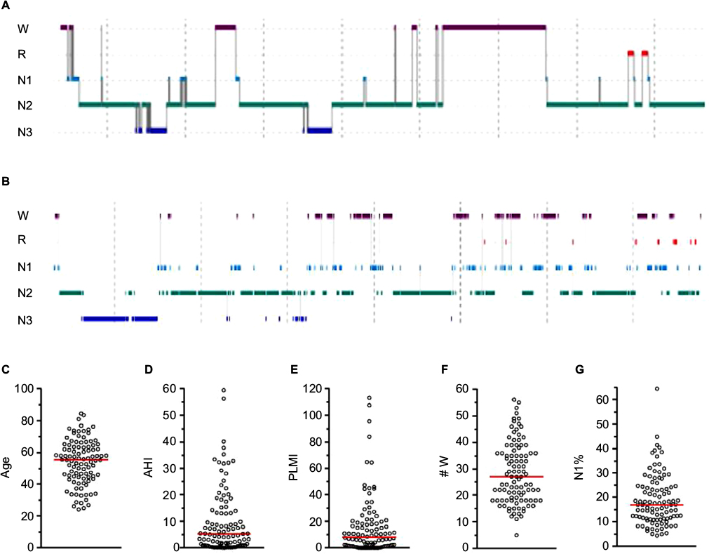Figure 3 Sleep efficiency: a limited view of heterogenous sleep physiology. Notes: (A and B) Hypnograms from different patients. (A) Sleep efficiency of 78.3%, associated with nine transitions to wake (age 23, male). (B) Sleep efficiency of 82%, associated with 46 transitions to wake (age 42, male). The Y-axis indicates scored stage; the time bar indicates 1 hour. (C–G) Distribution of n=100 individuals with essentially the same sleep efficiency values (79.5%–80.5%), but differ widely across other factors that potentially contribute to or signify sleep fragmentation (age, AHI, PLMI, # W, and N1%). Abbreviations: R, rapid eye movement sleep; N1–3, non-rapid eye movement stages 1–3; AHI, apnea–hypopnea index; PLMI, periodic limb movement index; # W, number of wake transitions.

Stage percentage is also an insensitive measure of fragmentation. We can consider two patients each with 120 minutes of stage REM within an 8-hour TST: one patient could have four REM blocks each lasting 30 continuous minutes, and the other could have four blocks interrupted by frequent brief transitions to wake or N1. Each patient’s summary report could indicate REM as 25% of TST, yet the two patterns of consolidation versus fragmentation are quite different and might imply distinct pathophysiology. This example illustrates that stage percentage does not capture fragmentation phenotypes associated with a known cause of fragmentation (OSA). Several alternative methods to stage percentage have been proposed, including bout duration histograms,³⁹ bout duration survival analysis,⁴⁰ and others.^41–44 Some have used multi-exponential transition models,⁴⁵ while others have used power-law approaches⁴⁶ to describe these skewed patterns. Even stage transition rates have proven useful where percentages have shown no discriminatory value.^47,48 Which one of these is the “best” descriptor of the distribution of sleep–wake stages remains open to discussion, although even statistically principled model selection methods may not distinguish true from alternative functions in simulation studies.⁴⁹

If stage percentage cannot distinguish individuals with no OSA from those with severe OSA (despite the obvious fragmentation seen visually), then it might be even less sensitive for comparing groups or evaluating interventions expected to have less dramatic impact on sleep. For example, in a study of yoga in healthy adults, distribution analysis revealed stage differences not evident by percentage analysis.⁵⁰ Likewise, stage percentage does not appear to distinguish patients with versus without misperception of TST, whereas differences were evident when stages were examined using bout distribution methods.⁵¹ One wonders how often initial analysis of stage percentage reveals little or no group differences, and deeper analysis of fragmentation is simply not pursued.

Phenotyping sleep apnea

The summary metric most commonly acted upon in clinical practice is the AHI, which is used to define the presence and severity of OSA. This event rate has become the cornerstone of diagnosis, a threshold index for insurance coverage of therapy, and a metric for inclusion and outcome of research trials. However, the OSA phenotype is much more heterogeneous than differences in AHI values might suggest, even if we put aside desaturation thresholds for scoring hypopneas^52–55 and the potential for night-to-night variability,^56–61 and other anatomical and physiological contributors.^62–64 OSA phenotypes can be described by extracting further details from routine PSG. For example, the severity of OSA often depends on sleep stage, and on body position, although a single night of PSG recording may not contain sufficient time in the different combinations of stage and position to make this determination.⁶⁵ Figure 4A illustrates an example of severe hypoxia to <60% during REM in a highly REM-dominant case, despite categorization as normal (AHI, 4.7) when the event rate is calculated over the full night. Figure 4B illustrates a strongly supine-dominant case, with normal AHI while sleeping in the lateral position, and very severe AHI while sleeping supine. The full-night AHI is the weighted average of these extremes, which happened to be 19.2 on this night. Had the person slept supine the whole time, or lateral the whole time (or if positions were not recorded), then very different conclusions about the presence and severity of OSA would likely be drawn. In this case, it is also interesting that REM dominance could not be assessed as only lateral REM was seen, and no apnea was present while lateral.

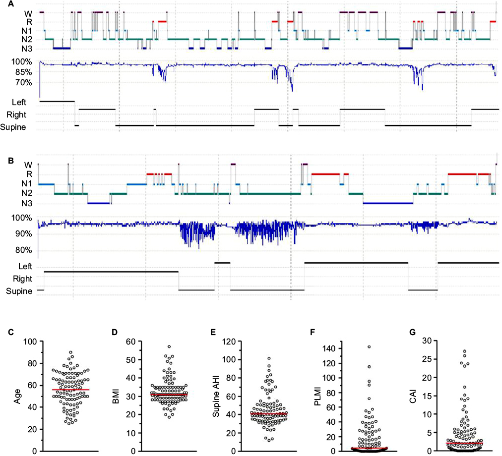Figure 4 AHI: a limited view of heterogenous sleep physiology Notes: (A and B) Hypnograms from different patients. (A) A case of REM-dominant obstruction with prominent hypoventilation pattern, resulting in a normal 4% AHI value (4.7 per hour), but a severe oxygen nadir of 57% (age 66; female; BMI, 35). (B) A case of supine-dominant sleep apnea, with a full night AHI in the moderate range (19.7 per hour), resulting from the weighted average of supine AHI of 62 and non-supine AHI of 0.9 (age 74; female; BMI, 21). (C–G) The distribution of n=100 individuals with similar 4% AHI values (30–35 per hour), but differ widely across other factors that shape the clinical phenotype and potentially therapy choices (age, BMI, supine AHI, PLMI, and CAI). Abbreviations: R, rapid eye movement sleep; N1–3, non-rapid eye movement stages 1–3; AHI, apnea–hypopnea index; BMI, body mass index; CAI, central apnea index; PLMI, periodic limb movement index; REM, rapid eye movement.

Which AHI is most relevant depends on several factors. For example, in a study of airway anatomy while supine in a scanner, the supine AHI might be most informative even if the individual never sleeps supine in the home. By contrast, in a study of clinical outcomes, the real-world AHI experienced by the patient is paramount: if the patient sleeps exclusively non-supine (and this can be demonstrated), then the lateral AHI is the relevant “phenotype” for that individual.

Characterizing supine dominance also has direct implications for clinical care. Patients with strong supine dominance may benefit by pursuing positional therapy. Much work exists in this area,⁶⁶ and devices to assist in position therapy exist in the consumer and prescription⁶⁷ spaces. Device-assisted therapy is important, especially because patients’ self-report of body position during sleep carries substantial uncertainty.⁶⁸ By contrast, REM dominance does not as easily translate into clinical care recommendations for therapy, but REM-dominant OSA has been increasingly linked to hypertension,⁶⁹ and thus might impact treatment motivation. Insufficient evidence exists regarding REM-suppressing agents as pharmacological therapy for OSA.⁷⁰

The heterogeneity in clinical features is apparent by examining a distinct set from our database with AHI in a very small range, 30–35 (n=100). In this group of very tightly clustered “severe” AHI cases, the age, body mass index (BMI), supine AHI, periodic limb movement index (PLMI), and central apnea index (Figure 4C–G) are each quite broadly dispersed. In addition, the distributions do not visually suggest obvious cutoffs or subgroups. In each case, clinical decisions might be distinct depending on where in the dispersion an individual resides in each category, and across categories; similar clinical sub-phenotypes have been discussed recently.⁶⁴ For example, an AHI of 30 in a slender 25-year-old with no periodic limb movements of sleep (PLMS) and a high supine AHI might have different treatment options or preferences (not to mention risks and outcomes) than an older obese patient with comorbid PLMS and increased central component. Clinically and in many research settings, severity categories span much larger AHI ranges, and are thus likely to have even more heterogeneity across these and other potentially important phenotypic axes (medications, alcohol, airway anatomy, etc).

Phenotyping insomnia

Insomnia is clinically defined entirely by self-reported symptoms. While research efforts impose cutoffs for sleep latency or WASO as inclusion criteria, in clinical practice the emphasis is on the severity of the complaint and the self-reported impact on daytime function rather than on numerical requirements of sleep parameters. Even in research settings, it can be challenging to demonstrate objective impact on daytime function,⁷¹ a reminder that chronic insomnia is not phenomenologically equivalent to experimental sleep restriction in healthy adults and the ensuing performance decrements. There is growing interest in using objective measures to study insomnia, with respect to the hyperarousal pathophysiology,⁷² as well as recent work indicating that it is the combination of insomnia and objective short sleep duration on PSG that is specifically associated with incident medical and psychiatric risk.^73,74

Despite the clinical reliance on self-report, extensive work highlights the challenges associated with the subjective experience of insomnia. As an example, the seemingly simple question of sleep duration, which forms the basis of nearly all epidemiological sleep research, depends on the demographics,⁷⁵ comorbid psychiatric disorders,^76,77 and comorbid sleep disorders.^78,79 In addition, within-individual analysis reveals some striking observations that when⁸⁰ and how⁸¹ sleep–wake durations are queried impacts patient responses. The prospect of internal inconsistency across query methods remains an important yet unresolved issue.

Prolonged sleep latency is a common complaint, and although it may seem a straightforward metric, it carries special challenges when understanding insomnia and specifically the misperception phenotype. Objective sleep latency measurement requires an operational definition, for which there is no gold standard. Although prior literature considered behavioral (non-EEG) approaches to identify sleep onset,^82,83 clinical reporting usually involves defining sleep onset by either the first epoch of any sleep or the first instance of a consolidated bout (e.g., 10 epochs) of uninterrupted sleep. Different definitions impact calculations and therefore experimental results. We can consider a patient with delayed sleep phase syndrome, who exhibits a 2-hour latency, but subsequent sleep was well consolidated, compared to an individual who spends the first 2 hours with fragmented brief transitions between wake and sleep, perhaps due to pain, and also has a 2-hour onset latency to persistent sleep. It is difficult to rationalize lumping these together under a definition of latency to persistent sleep (both are 2 hours).

For studies of misperception, the subjective sleep latency is compared to some definition of objective sleep onset; clearly, the definition of objective onset may impact the resulting calculation. We recently introduced a novel metric of sleep onset misperception that obviates the need to define objective sleep onset.⁵¹ The fundamental goal of quantifying sleep onset misperception is to capture how much sleep was misinterpreted as wake, and thus we calculated the total sleep duration occurring during the time between lights out and subjective onset. This also addresses a potential confound of assuming that onset misperception and TST misperception are independent. We can consider patients with objective sleep of 8-hour duration, with a 1-minute onset latency, who report subjectively a 4-hour onset latency and 4 hours of TST. Typically, these persons would be labeled as having both onset and total sleep misperception (4 hours each). However, if they had anchored their total sleep estimate to their own sleep latency estimate of 4 hours, then their 4-hour total sleep guess is an accurate estimate of TST occurring since they believed that they fell asleep. We recently showed that a substantial portion of patients would be reclassified if their misperception phenotype is based on the sleep during subjective latency, and the “corrected” total sleep misperception.⁵¹ Big datasets may allow further evaluation of misperception phenotype(s), which have not enjoyed consistent predictors in the prior literature.⁷⁷

Analysis and inference

Missing and erroneous database entries

Routine clinical data can be easily arranged in tabular format to facilitate an initial data evaluation. When these metrics are exported into spreadsheets with columns of features (and each row is one patient’s data), some straightforward cleaning methods can be implemented (Figure S3). Minimum, maximum, and counting commands can identify columns with missing data (e.g., count if empty), improperly formatted data (e.g., count if text is present), or implausible values (e.g., count if outside limit value). In some cases, such outliers or errors would be missed in routine plotting such as bar plots with standard deviations (SDs) or even box and whisker plots depending on whether outliers are plotted and how the axis ranges are chosen.

Several reasons for missing values are possible, including corrupted data (data were collected but were no longer accessible), collected but not recorded (paper copies fail to transfer to electronic database), and not collected. Some qualitative assessment of the distribution of variables from individuals who are missing at least one other entry in a data matrix can be useful.⁸⁴ Specific decisions regarding how to handle missing data points or error values are best handled by prespecifying a plan, which could involve excluding subjects or imputing missing values; more advanced discussions are available.⁸⁵

In some cases, missing values occur for appropriate reasons and the absence can be informative. For example, the REM AHI cannot be calculated if no REM sleep was observed during a PSG. Likewise, position dependence of OSA cannot be calculated for PSGs in which only supine position was observed. In these cases, removing such subjects might be favored over imputation.

Determining whether a given value is erroneous (versus a biologically plausible outlier) may depend on certain clues such as “impossible” values or known placeholders for missing data used by an acquisition software system. For example, negative values where only positive values are possible (e.g., age) are easily identified as both errors and outliers. Likewise, when letters are present instead of numbers, or where the value is out of range (e.g., ESS value of >24), these are also easily identified. In some examples (Figure S3), simply plotting the data identifies outliers. Database software such as Excel can easily show the maximum and minimum values for inspection of implausible values. As an example of errors not readily detected by the abovementioned methods, in our database the BMI and ESS are manually entered in adjacent fields, such that an out-of-range ESS value prompted inspection of the BMI as well, and in some cases it was shown by viewing the original data that these two values were interchanged (in this instance, the BMI value of 18 is plausible, and so it would not have been flagged as an outlier).

In some cases, we may still wish to exclude plausible data from analysis. Examples are related to stage- and position-specific metrics, wherein the amount of time spent in the condition of interest is the “sampling” problem, rather than the number of subjects. We may wish, for instance, to exclude people with minimal time in REM or minimal time spent sleeping supine, not just the zero time individuals, when calculating OSA dominance ratios or oxygen nadirs in REM. For AHI, the values could be artificially high (one apnea in one epoch), or artificially low (insufficient time spent in REM to manifest obstructions).

Distributions and plotting

Evaluating the distribution of individual variables can inform multiple aspects of analysis and inference. The most basic reason to understand the distribution is to decide what kind of statistical approach is most appropriate, such as whether continuous data are normally distributed or skewed in some manner, in which case data transformations to make the data distribution approximately normal (e.g., logarithmic transformation of positive-valued data) or nonparametric analysis methods may be preferred. Moreover, like plotting the raw data, evaluating the distribution using one of several techniques can also inform the approach to outliers, or the possibility of interesting biological heterogeneity. For example, multimodal distributions may imply that the population contains different sub-phenotypes that might be worthy of further investigation.

In our cohort, none of the variables passed statistical testing for normality, similar to prior work using the Sleep Heart Health Study database.⁸⁴ Of note, large samples may be highly “powered” to reject the null hypothesis of a normal distribution, even when the distribution appears nearly normal. Conversely, small samples are more likely to pass tests of normality, even if known to be non-normal.³⁹ Indeed, when we under-sampled the current dataset, there was increasing probability of passing tests for normality (Figure S4). Non-normal data can be handled by either nonparametric methods or transformation that render the data approximately normal. The challenge is as much statistical as biological: non-normal distributions may have phenotyping implications.

The method of plotting can impact the viewer’s impression of the data. Bar graphs with mean and SD or standard error of the mean (SEM) are commonly used, but these routine methods risk inadvertently concealing potentially important information. Figure 5 illustrates different plotting methods for groups of simulated data from known distributions. In the case of bar plots with SEM, casual inspection might give the false sense of reduced variance of the actual observations in the dataset (Figure 5A and B). This happens because the SEM is obtained by dividing the SD by the square root of the sample size, which makes error bars smaller. The SEM thus does not reflect variance in the data, but rather reflects the precision of the estimate of the mean value – one should not conflate the two.

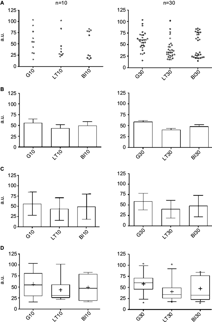Figure 5 Plotting views of three common distributions. Notes: Each row contains one plotting method for three distributions (G, LT skew, and BM). Each column contains a simulated sample size of n=10 (left) or n=30 (right). The individual points showed as dot plots (A) are given for comparison visually with more common views (B–D). Bar plots with SEM (B) appear quite similar across the simulated distributions. Similarly, plotting a bard with SD (C), there is little suggestion that three different distributions are shown. When plotted using box and whiskers, we observe clues of non-Gaussian distributions; here the box is the 25–75 percentile, the line is the median, + is the mean, and the whiskers are the 2.5–97.5 percentile. In each graph, the Y-axis is in a.u. Abbreviations: a.u., arbitrary units; BI, bimodal; G, Gaussian; LT, long tail; SD, standard deviation; SEM, standard error of the mean.

The SD, in contrast, reflects the dispersion in the data, and does not diminish with increasing sample size like the SEM. However, the SD may still be misleading in a bar graph when it is constructed from data with a non-normal distribution. Because the SD is by convention shown as symmetric bars around the mean (regardless of the actual underlying data distribution), viewers may be left with the potentially false impression of symmetric spread around the mean simply because of the display convention (Figure 5C). Sometimes the only clue in a bar graph that the population is skewed is that the SD value is greater than the mean value for a dataset that cannot take on negative values, which implies a long tail (i.e., non-normal). This is common, for example, in known skewed distributions such as AHI or sleep latency, where a value of, say, 15±18 would be interpreted as evidence of a long-tail non-normal distribution. Asymmetries and skew are visually evident in box and whisker plots (Figure 5D). However, even the box and whisker method can “hide” the distribution for unusually structured data, such as bimodal distributions, which would be phenotypically important to recognize.

Other techniques for visually assessing structure in populations include frequency histograms and cumulative distribution functions (CDFs). Histograms are used in Figure 6 to illustrate the distribution of TST, sleep efficiency, and the number of ≥30-second awakenings. The choice of bin size for histogram plots should consider the trade-off between granularity of the variable of interest, and sample size per bin. Too many bins cause the variable values to be either 0 or 1 in each bin, or to vary randomly from bin to bin due to sampling noise, and therefore offer little visual insight. Too few bins cause the underlying distribution to be overly smoothed. Histogram views can reveal outliers, suggest heterogeneity of the population, or inform selection of cutoff values (e.g., if a “valley” was seen between two modes within the data, suggests two populations). In contrast, the histograms shown in Figure 6 do not have clear “valleys” on visual inspection.

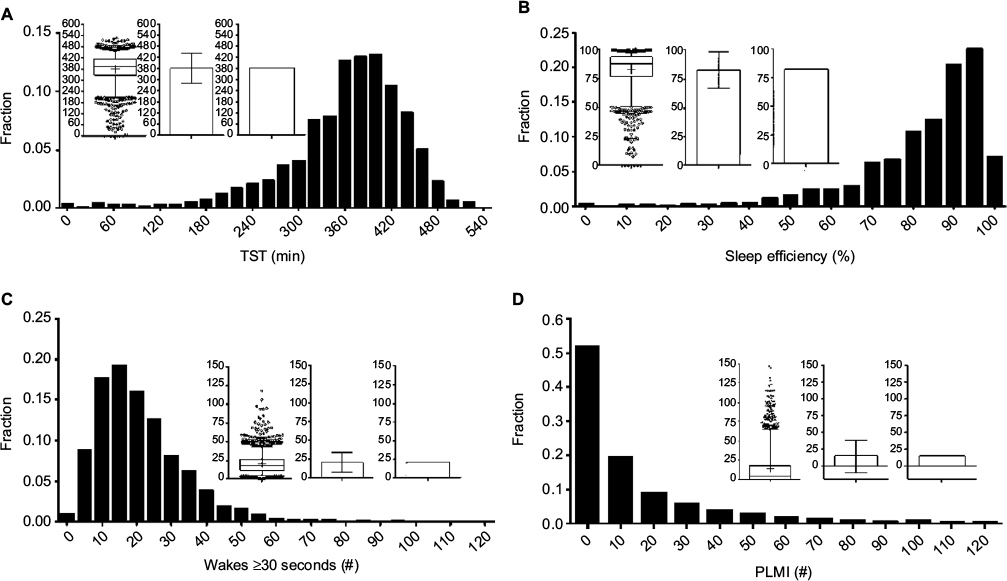Figure 6 Distributions of common PSG metrics. Notes: Each panel contains a frequency histogram of n=1835 PSGs for TST (A), efficiency (B), number of wake transitions (C), and PLMI (D). In each panel, the inlay graph contains three plots of the same distribution: box and whisker, bar with SD, and bar plot with SEM. The clearly skewed distributions are largely hidden by the bar plots, compared to the histogram and box and whisker views. Abbreviations: PLMI, periodic limb movement index; PSG, polysomnography; SEM, standard error of the mean; SD, standard deviation; TST, total sleep time.

CDF plots can also be informative, especially when comparing groups, or when the metric of interest is a threshold imposed upon a continuous variable. Unlike histograms, CDFs do not require specification of bin size; however, their visualization may be less intuitive. Figure 7 shows CDF plots for different sleep apnea metrics, such as position dependence of the AHI (Figure 7A) and of the central apnea index (Figure 7B). Figure 7C shows the distribution of time spent in different body positions during sleep. Threshold values can be evaluated visually, such as the portion of the population with at least 50% of the night spent supine (Figure 7C; ~60%), or who had a supine AHI value >30 (Figure 7A; ~20%).

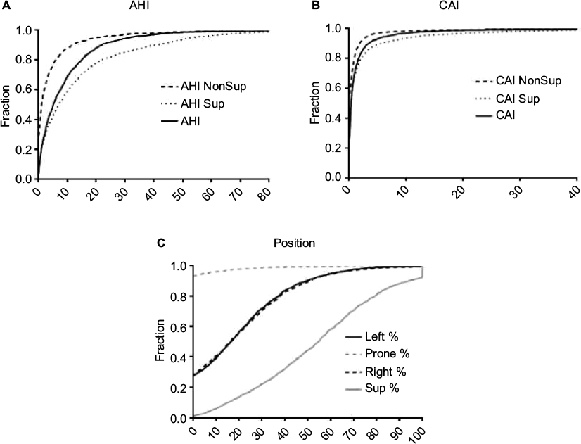Figure 7 Distribution of common sleep apnea PSG metrics. Notes: (A) CDFs for AHI, Sup AHI, and NonSup AHI; the Sup AHI values were higher as indicated by the slower rise of the CDF. (B) CDFs for CAI, which also showed some degree of position dependence. (C) A CDF of the percentage of sleep time spent in the four cardinal body positions; left and right showed similar distributions, while prone was not commonly observed. Abbreviations: AHI, apnea–hypopnea index; CAI, central apnea index; CDFs, cumulative distribution functions; NonSup, non-supine; PSG, polysomnography; Sup, supine.

Correlation analysis

One of the powerful approaches enabled by large datasets is investigating correlations between variables. Nonparametric (Spearman) correlation was performed between AHI and BMI, which are well known to be positively correlated. Taking the full cohort, the unadjusted Spearman’s R-value is ~0.25. Figure 8A shows the distribution of R-values for AHI versus BMI obtained when repeatedly analyzing randomly selected smaller subsets of the cohort. For the subgroups of the cohort, the range of R-values is larger for smaller sample sizes. In other words, smaller samples of the large cohort (n=1835) show much larger range of correlation values than the value of the whole set (~0.25). This variation includes more extreme R-values such as actually negative correlations in some cases (for the subsets of size n=10, n=20). Similar patterns are observed with another pair of parameters that showed a positive correlation in the large cohort (age and PLMI; Figure 8B).

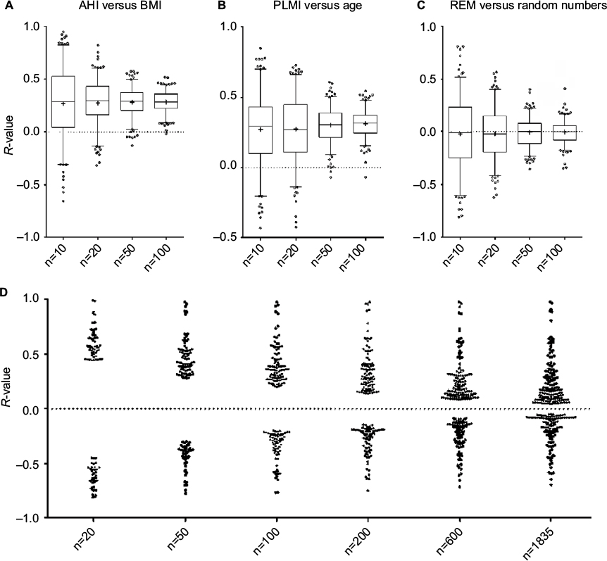Figure 8 Sample size impacts correlations calculated pairwise from PSG metrics. Notes: (A–C) Box and whisker plots of Spearman’s R-values obtained from random subsets of the full cohort (n=10, 20, 50, 100) for pairwise correlations: AHI with BMI (A), PLMI with age (B), and REM percentage with random numbers. Note the more extreme range of R-values (positive and negative) observed with smaller samples, and the wide range of observations even when correlating a PSG metric with uncorrelated random numbers. In (D), Spearman’s R-values were calculated for all pairwise correlations across 40 continuous variables (age, BMI, AHI, etc), but only those reaching a P-value <0.05 are shown. The resulting dot plots are shown across a range of sample sizes from n=20 up to the full cohort. Note that the range of significant R-values is strongly related to sample size, with only very large values reaching significance when the random subsets were small. Abbreviations: AHI, apnea–hypopnea index; BMI, body mass index; PLMI, periodic limb movement index; PSG, polysomnography; REM, rapid eye movement.

To emphasize the risks of under-sampled (small) data resulting in spurious findings using correlation analysis, we also demonstrate the R-values obtained when pairing REM% from the cohort with a vector of random numbers (Figure 8C). This plot clearly shows that significant correlations can occur, even with convincingly large R-values, with random data. These plots illustrate the concept that extreme values for statistical estimates (such as correlation coefficient or mean) are more common in under-sampled data. Most investigators reflexively think of “power” in the sense that lack of statistical significance when a true difference exists (type 2 error) could be a symptom of insufficient sample size. However, small sample sizes also harbor false-positive risk (type 1 error).

Large datasets can mitigate false-positive risks associated with the issue of small numbers mentioned earlier, except when the dataset is parsed into smaller and smaller subsets in data-mining queries of ever more specific subsets. Across all 41 continuous variables in the database, the threshold R-value for meeting significance was quite small when calculated from the entire cohort. The threshold for obtaining a significant R-value increases as progressively smaller subsets of the cohort are considered. Figure 8D illustrates how the “power” of the Spearman correlation calculated between any two pairs of variables decreases as the sample size decreases. In other words, when the entire cohort is considered, even quite small R-values in pairwise correlations meet significance criteria, because the large size essentially provides power to detect small correlations as significant. By contrast, small samples provide insufficient power to detect small correlations as statistically significant, and thus only large R-values meet significance criteria. This latter issue creates an interesting conundrum: because only large R-values can be significant when small datasets are considered, any significant correlation (whether true or false in reality) will necessarily have compelling-appearing R-values, which may overestimate the true R-value of that pair of variables, had a larger sample been utilized.

Sometimes, we may have prior information to help mitigate false inferences. Given the strong known relation between BMI and AHI, insignificant or paradoxical (negative associations) can be interpreted as false findings. However, in other cases, we may not have the benefit of strong prior knowledge, so assessing new data becomes more challenging.

Inferential pitfalls of small and large sample sizes

We have seen through empirical analyses and simulations that a spectrum of information and pitfalls are possible when working with large datasets. We now turn to illustrative examples from the literature in which large datasets may not be as explanatory as they appear. While there are many examples from which to choose, these example situations are representative of some key challenges.

Situation 1: when big data are still under-sampled

A recent study of more than 50 million pregnancies in the US sought to correlate adverse maternal and baby outcomes with OSA.⁸⁶ The study used billing codes from a massive registry to assign case labels for OSA. By this method, the prevalence of OSA in pregnancy was 3 per 10,000, approximately 100-fold lower than expected in this demographic. The discrepancy raises the possibility that the OSA coding is not just underestimating prevalence, but may also be biased, for example, toward the most severe or most symptomatic cases. If so, implications of any results based on these data greatly shrink in scope, as it they would apply only to the most severe cases of OSA or the most vulnerable or symptomatic individuals.

Situation 2: when big data explain little

While large sample sizes increase power, an associated risk involves the potential for being “overpowered” to detect very small correlations or group differences. We can observe this in the effect of modafinil on sleep latency of shift workers,⁸⁷ or in the relation of OSA severity with ESS.⁸⁸ A striking example of a very large sample supporting very small effects can be found in the analysis of mood rhythms detected in word analysis of more than 500 million tweets.⁸⁹ Relative change in day length was significantly related to positive affect, with an R-value of 1.2×10^-3, suggesting that the rhythm explained a fraction of a percent of affect fluctuations. These observations highlight the well-known but under-practiced mandate to focus scientific investigations on determining effect sizes, causal relationships, and establishing practical or clinical relevance, rather than focusing on simplistic binary questions at the heart of statistical significance testing.⁶

Situation 3: when big data are misinterpreted

The largest published study of home sleep testing was recently published, with the stated goal of determining if home testing was being used clinically in accordance with AASM standards.^90,91 The sample size of nearly 200,000 home tests is orders of magnitude larger than any prior home testing report. The authors concluded based on a high posttest probability of OSA (~80%) that indeed testing was in line with AASM guidelines. However, the AASM recommends that pretest probability (not posttest probability) should be >80% for at least moderate OSA (AHI >15). Bayes theorem tells us that the pretest probability of AHI >15 was <10% in the published cohort (and 50% if AHI >5 threshold is used),⁹² and thus the data actually support the opposite conclusion to that reached by the authors: home testing for OSA is being used too liberally, and not in line with the AASM guidance.

Another recent article⁹³ using administrative data from more than 2000 patients to derive a screening algorithm for OSA cases failed to recognize, by Bayes theorem, that their algorithm’s sensitivity and specificity were indicative of chance performance. One always needs to consider both sensitivity and specificity when evaluating any test. We use a simple calculation, the “rule of 100”, which can avoid this statistical fallacy: if the sensitivity and specificity of a test add to 100%, the probability of disease is unchanged by the result of the test (i.e., chance performance).

Conclusion

Clinical databases have important strengths that can support big data research goals. Clinical data contain diversity and heterogeneity that may be specifically excluded in clinical trial databases, which are often designed to reduce sources of variability that can be detrimental to power calculations and outcome testing. Clinical databases are more likely to reflect “real-world” variation in clinical phenotypes. This can be important for testing whether predictive algorithms can generalize across a diversity of clinical phenotypes. In addition, heterogeneous sets may be more amenable to clustering and other exploratory methods that allow discovery of new phenotypes that can be explored in subsequent prospective studies. From a resource utilization standpoint, clinical databases are a natural extension of already acquired data supporting patient care, which allows valuable and limited resources to be applied at the analysis phase.

Despite these advantages, certain limitations must be recognized. Academic centers may have different referral biases, for example, being enriched for complicated cases. Although most clinical laboratories have standardized physiological recording protocols, the collection of self-reported clinical information may not be standardized. Variation across recording and scoring technologists may contribute heterogeneity despite quality efforts required in accredited laboratories. Centralized scoring common to large clinical trials may not be practical for clinical databases.

Large sleep datasets offer the opportunity to pursue complex phenotyping exploration, and to detect scientifically or clinically interesting differences or patterns in health and disease. Despite the clear advantages, analysis of big data in sleep medicine also carries risks. Understanding common pitfalls can help mitigate the risks, whether one is conducting the analysis or reviewing publications involving big data. Ideally, what is learned from population-level big data efforts can then inform individual clinical care decisions. In an era when insurance restrictions are driving at-home limited channel alternatives, these efforts will be critical to elaborate and justify the current and possibly more advanced future use of PSG for clinical care. The era of big data in sleep medicine is poised to provide unprecedented insights, especially as it coincides with massive shifts in reimbursement and availability of laboratory-based PSG.

Disclosure

Dr Matt T Bianchi has received funding from the Department of Neurology, Massachusetts General Hospital, the Center for Integration of Medicine and Innovative Technology, the Milton Family Foundation, the MGH-MIT Grand Challenge, and the American Sleep Medicine Foundation. He has a pending patent on a sleep wearable device, received research funding from MC10 Inc and Insomnisolv Inc, has a consulting agreement with McKesson Health and International Flavors and Fragrances, serves as a medical monitor for Pfizer, and has provided expert testimony in sleep medicine. Dr M Brandon Westover receives funding from NIH-NINDS (1K23NS090900), the Rappaport Foundation, and the Andrew David Heitman Neuroendovascular Research Fund. The authors report no other conflicts of interest in this work.

References

1.		Dean DA, Goldberger AL, Mueller R, et al. Scaling up scientific discovery in sleep medicine: the National Sleep Research Resource. Sleep. 2016;39(5):1151–1164.
2.		O’Reilly C, Gosselin N, Carrier J, Nielsen T. Montreal Archive of Sleep Studies: an open-access resource for instrument benchmarking and exploratory research. J Sleep Res. 2014;23(6):628–635.
3.		Douglass C [webpage on the Internet]. American Sleep Apnea Association and IBM Launch Patient-led Sleep Study App. 2016. Available from: http://www-03.ibm.com/press/us/en/pressrelease/49275.wss. Accessed April 4, 2016.
4.		Falk R, Greenbaum CW. Significance tests die hard: the amazing persistence of a probabilistic misconception. Theory Psychol. 1995;5:75–98.
5.		Ioannidis JP. Why most published research findings are false. PLoS Med. 2005;2(8):e124.
6.		Westover MB, Westover KD, Bianchi MT. Significance testing as perverse probabilistic reasoning. BMC Med. 2011;9:20.
7.		Gill J. The insignificance of null hypothesis significance testing. Polit Res Q. 1999;52(3):647–674.
8.		Goodman SN. Toward evidence-based medical statistics. 1: the P value fallacy. Ann Intern Med. 1999;130(12):995–1004.
9.		Button KS, Ioannidis JP, Mokrysz C, et al. Power failure: why small sample size undermines the reliability of neuroscience. Nat Rev Neurosci. 2013;14(5):365–376.
10.		Nuzzo R. Scientific method: statistical errors. Nature. 2014;506(7487):150–152.
11.		Bianchi MT, Phillips AJ, Wang W, Klerman EB. Statistics for Sleep and Biological Rhythms Research: from distributions and displays to correlation and causation. J Biol Rhythms. Epub 2016 Oct 24.
12.		Klerman EB, Wang W, Phillips AJ, Bianchi MT. Statistics for Sleep and Biological Rhythms Research: longitudinal analysis of biological rhythms data. J Biol Rhythms. Epub 2016 Oct 24.
13.		Huck S. Statistical Misconceptions. Abingdon-on-Thames: Routledge; 2008.
14.		Ziliak ST, McCloskey DN. The Cult of Statistical Significance. Ann Arbor, MI: The University of Michigan Press; 2008.
15.		Reinhart A. Statistics Done Wrong: The Woefully Complete Guide. San Francisco, CA: No Starch Press; 2015.
16.		Redline S, Dean D 3rd, Sanders MH. Entering the era of “big data”: getting our metrics right. Sleep. 2013;36(4):465–469.
17.		Silber MH, Ancoli-Israel S, Bonnet MH, et al. The visual scoring of sleep in adults. J Clin Sleep Med. 2007;3(2):121–131.
18.		Babadi B, Brown EN. A review of multitaper spectral analysis. IEEE Trans Biomed Eng. 2014;61(5):1555–1564.
19.		Stein PK, Pu Y. Heart rate variability, sleep and sleep disorders. Sleep Med Rev. 2012;16(1):47–66.
20.		Citi L, Bianchi MT, Klerman EB, Barbieri R. Instantaneous monitoring of sleep fragmentation by point process heart rate variability and respiratory dynamics. Conf Proc IEEE Eng Med Biol Soc. 2011;2011:7735–7738.
21.		Thomas RJ, Mietus JE, Peng CK, et al. Differentiating obstructive from central and complex sleep apnea using an automated electrocardiogram-based method. Sleep. 2007;30(12):1756–1769.
22.		Chervin RD, Shelgikar AV, Burns JW. Respiratory cycle-related EEG changes: response to CPAP. Sleep. 2012;35(2):203–209.
23.		Chervin RD, Burns JW, Ruzicka DL. Electroencephalographic changes during respiratory cycles predict sleepiness in sleep apnea. Am J Respir Crit Care Med. 2005;171(6):652–658.
24.		McKinney SM, Dang-Vu TT, Buxton OM, Solet JM, Ellenbogen JM. Covert waking brain activity reveals instantaneous sleep depth. PLoS One. 2011;6(3):e17351.
25.		Dang-Vu TT, McKinney SM, Buxton OM, Solet JM, Ellenbogen JM. Spontaneous brain rhythms predict sleep stability in the face of noise. Curr Biol. 2010;20(15):R626–R627.
26.		Sforza E, Pichot V, Barthelemy JC, Haba-Rubio J, Roche F. Cardiovascular variability during periodic leg movements: a spectral analysis approach. Clin Neurophysiol. 2005;116(5):1096–1104.
27.		Sforza E, Juony C, Ibanez V. Time-dependent variation in cerebral and autonomic activity during periodic leg movements in sleep: implications for arousal mechanisms. Clin Neurophysiol. 2002;113(6):883–891.
28.		Aritake S, Blackwell T, Peters KW, et al. Prevalence and associations of respiratory-related leg movements: the MrOS sleep study. Sleep Med. 2015;16(10):1236–1244.
29.		Buxton OM, Ellenbogen JM, Wang W, et al. Sleep disruption due to hospital noises: a prospective evaluation. Ann Intern Med. 2012;157(3):170–179.
30.		Winkelman JW. The evoked heart rate response to periodic leg movements of sleep. Sleep. 1999;22(5):575–580.
31.		Younes M, Hanly PJ. Immediate postarousal sleep dynamics: an important determinant of sleep stability in obstructive sleep apnea. J Appl Physiol (1985). 2016;120(7):801–808.
32.		Azarbarzin A, Ostrowski M, Hanly P, Younes M. Relationship between arousal intensity and heart rate response to arousal. Sleep. 2014;37(4):645–653.
33.		Ohayon MM, Carskadon MA, Guilleminault C, Vitiello MV. Meta-analysis of quantitative sleep parameters from childhood to old age in healthy individuals: developing normative sleep values across the human lifespan. Sleep. 2004;27(7):1255–1273.
34.		Mayers AG, Baldwin DS. Antidepressants and their effect on sleep. Hum Psychopharmacol. 2005;20(8):533–559.
35.		Sullivan SS. Insomnia pharmacology. Med Clin North Am. 2010;94(3):563–580.
36.		Wesensten NJ, Balkin TJ, Belenky G. Does sleep fragmentation impact recuperation? A review and reanalysis. J Sleep Res. 1999;8(4):237–245.
37.		Thomas RJ. Sleep fragmentation and arousals from sleep-time scales, associations, and implications. Clin Neurophysiol. 2006;117(4):707–711.
38.		Bianchi MT, Thomas RJ. Technical advances in the characterization of the complexity of sleep and sleep disorders. Prog Neuropsychopharmacol Biol Psychiatry. 2013;45:277–286.
39.		Bianchi MT, Cash SS, Mietus J, Peng CK, Thomas R. Obstructive sleep apnea alters sleep stage transition dynamics. PLoS One. 2010;5(6):e11356.
40.		Norman RG, Scott MA, Ayappa I, Walsleben JA, Rapoport DM. Sleep continuity measured by survival curve analysis. Sleep. 2006;29(12):1625–1631.
41.		Swihart BJ, Caffo B, Bandeen-Roche K, Punjabi NM. Characterizing sleep structure using the hypnogram. J Clin Sleep Med. 2008;4(4):349–355.
42.		Laffan A, Caffo B, Swihart BJ, Punjabi NM. Utility of sleep stage transitions in assessing sleep continuity. Sleep. 2010;33(12):1681–1686.
43.		Klerman EB, Davis JB, Duffy JF, Dijk DJ, Kronauer RE. Older people awaken more frequently but fall back asleep at the same rate as younger people. Sleep. 2004;27(4):793–798.
44.		Kishi A, Struzik ZR, Natelson BH, Togo F, Yamamoto Y. Dynamics of sleep stage transitions in healthy humans and patients with chronic fatigue syndrome. Am J Physiol Regul Integr Comp Physiol. 2008;294(6):R1980–R1987.
45.		Bianchi MT, Eiseman NA, Cash SS, Mietus J, Peng CK, Thomas RJ. Probabilistic sleep architecture models in patients with and without sleep apnea. J Sleep Res. 2012;21(3):330–341.
46.		Lo CC, Chou T, Penzel T, et al. Common scale-invariant patterns of sleep-wake transitions across mammalian species. Proc Natl Acad Sci U S A. 2004;101(50):17545–17548.
47.		Haba-Rubio J, Ibanez V, Sforza E. An alternative measure of sleep fragmentation in clinical practice: the sleep fragmentation index. Sleep Med. 2004;5(6):577–581.
48.		Bianchi MT, Kim S, Galvan T, White DP, Joffe H. Nocturnal hot flashes: relationship to objective awakenings and sleep stage transitions. J Clin Sleep Med. 2016;12(7):1003–1009.
49.		Chu-Shore J, Westover MB, Bianchi MT. Power law versus exponential state transition dynamics: application to sleep-wake architecture. PLoS One. 2010;5(12):e14204.
50.		Kudesia RS, Bianchi MT. Decreased nocturnal awakenings in young adults performing Bikram yoga: a Low-Constraint Home Sleep Monitoring Study. ISRN Neurol. 2012;2012:153745.
51.		Saline A, Goparaju B, Bianchi MT. Sleep fragmentation does not explain misperception of latency or total sleep time. J Clin Sleep Med. 2016;12(9):1245–1255.
52.		Grigg-Damberger MM. The AASM scoring manual: a critical appraisal. Curr Opin Pulm Med. 2009;15(6):540–549.
53.		Parrino L, Ferri R, Zucconi M, Fanfulla F. Commentary from the Italian Association of Sleep Medicine on the AASM manual for the scoring of sleep and associated events: for debate and discussion. Sleep Med. 2009;10(7):799–808.
54.		Redline S, Budhiraja R, Kapur V, et al. The scoring of respiratory events in sleep: reliability and validity. J Clin Sleep Med. 2007;3(2):169–200.
55.		Ruehland WR, Rochford PD, O’Donoghue FJ, Pierce RJ, Singh P, Thornton AT. The new AASM criteria for scoring hypopneas: impact on the apnea hypopnea index. Sleep. 2009;32(2):150–157.
56.		Aarab G, Lobbezoo F, Hamburger HL, Naeije M. Variability in the apnea-hypopnea index and its consequences for diagnosis and therapy evaluation. Respiration. 2009;77(1):32–37.
57.		Ahmadi N, Shapiro GK, Chung SA, Shapiro CM. Clinical diagnosis of sleep apnea based on single night of polysomnography vs. two nights of polysomnography. Sleep Breath. 2009;13(3):221–226.
58.		Le Bon O, Hoffmann G, Tecco J, et al. Mild to moderate sleep respiratory events: one negative night may not be enough. Chest. 2000;118(2):353–359.
59.		Levendowski D, Steward D, Woodson BT, Olmstead R, Popovic D, Westbrook P. The impact of obstructive sleep apnea variability measured in-lab versus in-home on sample size calculations. Int Arch Med. 2009;2(1):2.
60.		Mosko SS, Dickel MJ, Ashurst J. Night-to-night variability in sleep apnea and sleep-related periodic leg movements in the elderly. Sleep. 1988;11(4):340–348.
61.		Stepnowsky CJ Jr, Orr WC, Davidson TM. Nightly variability of sleep-disordered breathing measured over 3 nights. Otolaryngol Head Neck Surg. 2004;131(6):837–843.
62.		Riha RL, Gislasson T, Diefenbach K. The phenotype and genotype of adult obstructive sleep apnoea/hypopnoea syndrome. Eur Respir J. 2009;33(3):646–655.
63.		Subramani Y, Singh M, Wong J, Kushida CA, Malhotra A, Chung F. Understanding phenotypes of obstructive sleep apnea: applications in anesthesia, surgery, and perioperative medicine. Anesth Analg. 2017;124(1):179–191.
64.		Zinchuk AV, Gentry MJ, Concato J, Yaggi HK. Phenotypes in obstructive sleep apnea: a definition, examples and evolution of approaches. Sleep Med Rev. Epub 2016 Oct 12.
65.		Eiseman NA, Westover MB, Ellenbogen JM, Bianchi MT. The impact of body posture and sleep stages on sleep apnea severity in adults. J Clin Sleep Med. 2012;8(6):655A–666A.
66.		de Vries N. Positional Therapy in Obstructive Sleep Apnea. Berlin: Springer; 2014.
67.		Levendowski DJ, Seagraves S, Popovic D, Westbrook PR. Assessment of a neck-based treatment and monitoring device for positional obstructive sleep apnea. J Clin Sleep Med. 2014;10(8):863–871.
68.		Russo K, Bianchi MT. How reliable is self-reported body position during sleep? J Clin Sleep Med. 2016;12(1):127–128.
69.		Appleton SL, Vakulin A, Martin SA, et al. Hypertension is associated with undiagnosed OSA during rapid eye movement sleep. Chest. 2016;150(3):495–505.
70.		Morgenthaler TI, Kapen S, Lee-Chiong T, et al. Practice parameters for the medical therapy of obstructive sleep apnea. Sleep. 2006;29(8):1031–1035.
71.		Shekleton JA, Rogers NL, Rajaratnam SM. Searching for the daytime impairments of primary insomnia. Sleep Med Rev. 2010;14(1):47–60.
72.		Bonnet MH, Arand DL. Hyperarousal and insomnia: state of the science. Sleep Med Rev. 2010;14(1):9–15.
73.		Vgontzas AN, Fernandez-Mendoza J, Liao D, Bixler EO. Insomnia with objective short sleep duration: the most biologically severe phenotype of the disorder. Sleep Med Rev. 2013;17(4):241–254.
74.		Fernandez-Mendoza J, Shea S, Vgontzas AN, Calhoun SL, Liao D, Bixler EO. Insomnia and incident depression: role of objective sleep duration and natural history. J Sleep Res. 2015;24(4):390–398.
75.		Kurina LM, McClintock MK, Chen JH, Waite LJ, Thisted RA, Lauderdale DS. Sleep duration and all-cause mortality: a critical review of measurement and associations. Ann Epidemiol. 2013;23(6):361–370.
76.		Fernandez-Mendoza J, Calhoun SL, Bixler EO, et al. Sleep misperception and chronic insomnia in the general population: role of objective sleep duration and psychological profiles. Psychosom Med. 2011;73(1):88–97.
77.		Harvey AG, Tang NK. (Mis)perception of sleep in insomnia: a puzzle and a resolution. Psychol Bull. 2012;138(1):77–101.
78.		Vanable PA, Aikens JE, Tadimeti L, Caruana-Montaldo B, Mendelson WB. Sleep latency and duration estimates among sleep disorder patients: variability as a function of sleep disorder diagnosis, sleep history, and psychological characteristics. Sleep. 2000;23(1):71–79.
79.		Bianchi MT, Williams KL, McKinney S, Ellenbogen JM. The subjective-objective mismatch in sleep perception among those with insomnia and sleep apnea. J Sleep Res. 2013;22(5):557–568.
80.		Fichten CS, Creti L, Amsel R, Bailes S, Libman E. Time estimation in good and poor sleepers. J Behav Med. 2005;28(6):537–553.
81.		Alameddine Y, Ellenbogen JM, Bianchi MT. Sleep-wake time perception varies by direct or indirect query. J Clin Sleep Med. 2015;11(2):123–129.
82.		Ogilvie RD. The process of falling asleep. Sleep Med Rev. 2001;5(3):247–270.
83.		Prerau MJ, Hartnack KE, Obregon-Henao G, et al. Tracking the sleep onset process: an empirical model of behavioral and physiological dynamics. PLoS Comput Biol. 2014;10(10):e1003866.
84.		Eiseman NA, Westover MB, Mietus JE, Thomas RJ, Bianchi MT. Classification algorithms for predicting sleepiness and sleep apnea severity. J Sleep Res. 2012;21(1):101–112.
85.		Cismondi F, Fialho AS, Vieira SM, Reti SR, Sousa JM, Finkelstein SN. Missing data in medical databases: impute, delete or classify? Artif Intell Med. 2013;58(1):63–72.
86.		Louis JM, Mogos MF, Salemi JL, Redline S, Salihu HM. Obstructive sleep apnea and severe maternal-infant morbidity/mortality in the United States, 1998–2009. Sleep. 2014;37(5):843–849.
87.		Czeisler CA, Walsh JK, Roth T, et al. Modafinil for excessive sleepiness associated with shift-work sleep disorder. N Engl J Med. 2005;353(5):476–486.
88.		Gottlieb DJ, Whitney CW, Bonekat WH, et al. Relation of sleepiness to respiratory disturbance index: the Sleep Heart Health Study. Am J Respir Crit Care Med. 1999;159(2):502–507.
89.		Golder SA, Macy MW. Diurnal and seasonal mood vary with work, sleep, and daylength across diverse cultures. Science. 2011;333(6051):1878–1881.
90.		Collop NA, Tracy SL, Kapur V, et al. Obstructive sleep apnea devices for out-of-center (OOC) testing: technology evaluation. J Clin Sleep Med. 2011;7(5):531–548.
91.		Collop NA, Anderson WM, Boehlecke B, et al. Clinical guidelines for the use of unattended portable monitors in the diagnosis of obstructive sleep apnea in adult patients. Portable Monitoring Task Force of the American Academy of Sleep Medicine. J Clin Sleep Med. 2007;3(7):737–747.
92.		Bianchi MT. Evidence that home apnea testing does not follow AASM practice guidelines – or Bayes’ theorem. J Clin Sleep Med. 2015;11(2):189.
93.		Laratta CR, Tsai WH, Wick J, Pendharkar SR, Johannson KA, Ronksley PE. Validity of administrative data for identification of obstructive sleep apnea. J Sleep Res. Epub 2016 Oct 20.

Supplementary materials

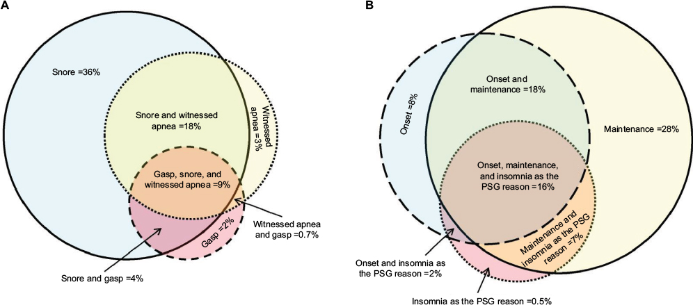Figure S1 Overlap of symptoms associated with sleep apnea and insomnia. Notes: (A) Venn diagram of symptoms related to sleep apnea: snoring (solid line, blue fill), gasping arousals (dashed line, red fill), and witnessed apnea (dotted line, yellow fill). The n-value (sample size) for each category: snoring only =656; snoring and witnessed apnea =337; gasping and snoring and witnessed apnea =166; snoring and gasping =70; gasping only =34; witnessed apnea and gasping =13; witnessed apnea only =61. (B) Venn diagram of insomnia symptoms: onset (dashed line, blue fill), maintenance (solid line, yellow fill), and listing insomnia as the reason for PSG (dotted line, red fill). The n-values for each category: onset only =148; onset and maintenance =331; maintenance only =521; maintenance and listing insomnia as the reason for PSG =121; listing insomnia as the reason for PSG but no other symptoms were indicated =10; onset and maintenance insomnia and listing insomnia as the reason for PSG =288; onset and listing insomnia as the reason for PSG =38. Abbreviation: PSG, polysomnography.

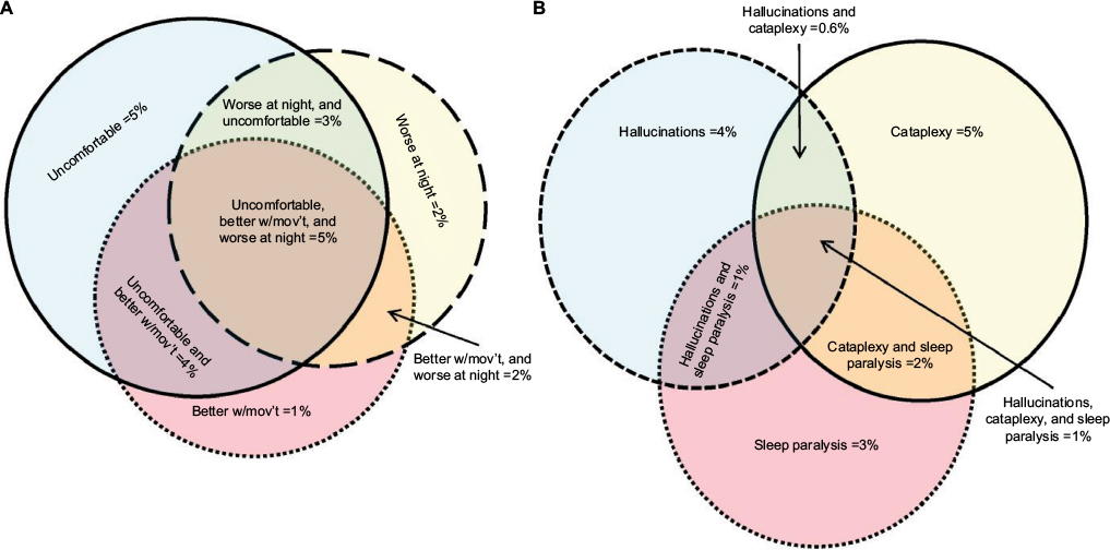Figure S2 Overlap of symptoms associated with restless legs and with narcolepsy. Notes: (A) Venn diagram of symptoms related to restless legs: uncomfortable sensation in the legs (solid line, blue fill), better with movement (w/mov’t) (dotted line, red fill), and worse at night (dashed line, yellow fill). The n-values (sample sizes) for each category: uncomfortable sensation alone =94; uncomfortable and better with movement =72; better with movement alone =26; better with movement and worse at night =33; uncomfortable and better with movement and worse at night =90; worse at night alone =42; uncomfortable and worse at night =49. (B) Venn diagram of narcolepsy symptoms: peri-sleep hallucinations (dashed line, blue fill), sleep paralysis (dotted line, red fill), and cataplexy (solid line, yellow fill). The n-values for each category: hallucinations alone =77; hallucinations and cataplexy =11; cataplexy alone =82; hallucinations and sleep paralysis =21; hallucinations and cataplexy and sleep paralysis =17; cataplexy and sleep paralysis =30; sleep paralysis alone =59.

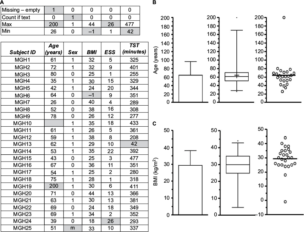Figure S3 Assessing missing data. Notes: (A) An example of missing data, outliers, and data reversals (subject code MGH24: the BMI and ESS scores are switched, but the error codes are only implausible for ESS), indicated by gray shading. Column statistics (maximum, minimum, count if text, and missing cell entries) can be helpful to alert potential anomalous data. (B) The age variable from (A) represented as a bar plot with SD, a box and whisker plot, and a dot plot; the outlier is not evident in the bar with SD. (C) The BMI variable from (A); similarly, the presence of an outlier is not evident in the bar with SD, and none hint at the switch with ESS because the erroneous value was plausible. In the Sex column in (A), 0= female and 1= male. Abbreviations: BMI, body mass index; ESS, Epworth Sleepiness Scale; m, male; Max, maximum; Min, minimum; SD, standard deviation; Subj, subject; TST, total sleep time.

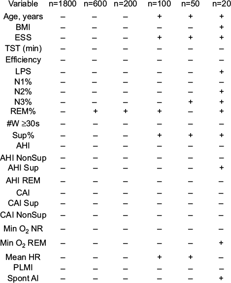Figure S4 Normality testing results vary by sample size. Notes: The variables listed were tested for normality (D’Agostino–Pearson test), with “–” indicating failed testing for normality and “+” indicating passed testing for normality. The columns indicate the sample size of random subsets of the full dataset, with none passing when the sample size was 1800. Abbreviations: AHI, apnea–hypopnea index; AHI NonSup, apnea–hypopnea index in non-supine; AHI Sup, apnea–hypopnea index in supine; BMI, body mass index; CAI, central apnea index; CAI NonSup, central apnea index in non-supine; CAI Sup, central apnea index in supine; ESS, Epworth Sleepiness Scale; LPS, latency to persistent sleep; mean HR, mean heart rate; Min O2 NR, minimum oxygen in non-REM; N1–3, non-REM stages 1–3; Min O2 REM, minimum oxygen in REM; PLMI, periodic limb movement index; REM, rapid eye movement; Spont AI, spontaneous apnea index; Sup%, supine percentage; TST, total sleep time; #W≥30s, number of wakes >30 seconds.