")
Back to Journals » Therapeutics and Clinical Risk Management » Volume 11
Bayesian imperfect information analysis for clinical recurrent data
Received 30 April 2014
Accepted for publication 12 August 2014
Published 19 December 2014 Volume 2015:11 Pages 17—26
DOI https://doi.org/10.2147/TCRM.S67011
Checked for plagiarism Yes
Review by Single anonymous peer review
Peer reviewer comments 3
Editor who approved publication: Professor Garry Walsh
Chih-Kuang Chang,1 Chi-Chang Chang2
1Department of Cardiology, Jen-Ai Hospital, Dali District, Taichung, Taiwan; 2School of Medical Informatics, Chung Shan Medical University, Information Technology Office of Chung Shan Medical University Hospital, Taichung, Taiwan
Abstract: In medical research, clinical practice must often be undertaken with imperfect information from limited resources. This study applied Bayesian imperfect information-value analysis to realistic situations to produce likelihood functions and posterior distributions, to a clinical decision-making problem for recurrent events. In this study, three kinds of failure models are considered, and our methods illustrated with an analysis of imperfect information from a trial of immunotherapy in the treatment of chronic granulomatous disease. In addition, we present evidence toward a better understanding of the differing behaviors along with concomitant variables. Based on the results of simulations, the imperfect information value of the concomitant variables was evaluated and different realistic situations were compared to see which could yield more accurate results for medical decision-making.
Keywords: Bayesian value-of-information, recurrent events, chronic granulomatous disease
Introduction
Recurrent events data on chronic diseases permeate medical fields, hence it is very important to have suitable models and approaches for statistical analyses.1 Published literature on recurrent events, (include childhood infectious diseases;2 cervical cancer;3 colon cancer;4,5 clinical trials;6 and dose-finding7). Treatment of recurrent events is still a clinical challenge today. A central problem in recurrent survival modeling is determining the distribution of the time [0,T]; that is, the first event defines the population of interest and initiates the start of the time interval at t=0, while the second event is the event of interest and terminates the time interval at time t=T. Researchers focused on an observed point process, along with fixed concomitant variables.7 Among these variables, the primary ones are age (time elapsed since birth) and/or time elapsed since an important event (eg, commencement of illness, date of operation), and they are regarded as being of prime interest.8 It is often desirable to assess the relationship between mortality and these primary concomitant variables. In general, any of the concomitant variables can be discrete or continuous. Among continuous variables, age plays an important role, and it is almost always recorded as the date of entry. Other variables, including recurrent events, are usually not only age dependent, but also vary from time to time, somewhat irregularly, for the same individual. The said variables are usually measured at the beginning of, and also periodically during the course of, a clinical trials. It is very important to note that, if the model involves values of concomitant variables measured after treatment has commenced, and these values are affected by the treatment itself, there is a need for special care in the interpretation of the results of analyses.9,10 At the time of decision-making, the measure probability of future deterioration of disease, which is likely to be uncertain, is of primary interest for the clinical physician.11
Generally, gathering additional data will not always be economical. Pratt et al described:
[...] the increase in utility which would result if the decision maker learned that Z=z (additional information). The utility which results from learning that Z=z will be called the value of the information z.12
Wendt stated:
Information that will reduce the risk of a decision may be costly in time, effort, or money. The maximum amount that should be invested in the information – its fair cost – depends upon payoffs and prior probabilities of the hypotheses.13
In Bayesian decision theory, the payoff is the loss function, and the diagnosticity of the data source is represented by the likelihood function. Bayesian decision theory and an analysis of the value of information can be used to decide whether the evidence in an economic study is “sufficient” substantiation. However, collecting additional clinical recurrent data will not always be low cost. According to Chang and Cheng,14 which was based on the assumption that we could obtain perfect information about the concomitant variables of interest.
In medical research, clinical practice must often be undertaken with imperfect information from observational studies and limited resources (these reasons include, the diagnostic accuracy of infectious diseases;15 the sample size calculations for randomized clinical trials;16 health tracking information management for outpatients;17 estimating diagnostic accuracy of multiple binary tests;18 or the reference standard for panel diagnosis19). In this light, it seems more reasonable to assume that the information we collect will be imperfect. In such situations, it becomes important to choose the optimal sample size for recurrent data. Since more extensive sampling will give us information that is more nearly perfect, but only at an increased cost, knowing the value of information is a good basis for determining the optimal amount of information to collect.20,21 In seeking optimal amount of information, both “qualitative information” and “quantitative information” are considered. Qualitative information does not come from actual failure data, but from expert opinion or past experience. In such cases, no actual failure data will be available for use in Bayesian value of information analysis. On the other hand, quantitative information is considered to be sample information that comes from an actual failure dataset. In this case, the nonhomogeneous Poisson process (NHPP) data can be transformed to equivalent homogeneous Poisson process data. According to the empirical investigation of Chang and Cheng,14 this paper discusses the decision analysis procedure when the collected information is assumed to be imperfect.
Imperfect information analysis for survival model parameters
This section describes the processes of prior and posterior decision making for each of the three clinical failure models (linear, power law, and exponential) when only imperfect information is available.1 Further, Figure 1 is a flowchart of the proposed Bayesian procedure. In this case, the additional information is imperfect, additional data or other information can be obtained by more detailed analysis of the existing data. However, before collecting additional information, one must investigate its possible outcomes and costs of each candidate sampling plan, to determine whether collecting additional information is worthwhile and also which sampling plan is the best in terms of cost-effectiveness.
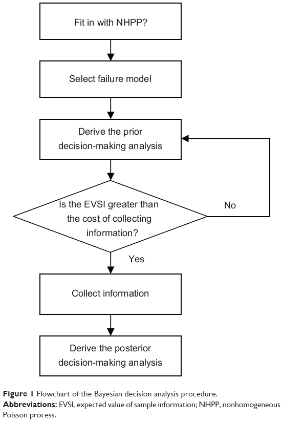 | Figure 1 Flowchart of the Bayesian decision analysis procedure. |
The case of unknown λ0 and known β
Two parameters, λ0 (the scale factor) and β (the aging rate), are useful in characterizing different clinical cases. The known aging processes about β and the information we collect for λ0 may be imperfect. Detailed root cause analysis could conceivably provide information only about λ0; for example, by revealing whether the root causes of observed failures were gene-related. Following discussion is based on NHPP.20
Qualitative information analysis
Collected information may not come from actual clinical failure data, but from physician opinions or past experiences. In such cases, it is still important to develop a procedure to take into account other types of information. Suppose ω is the estimated quantity of interest, which can be either the scale factor λ0 itself or some function of it (eg, M, the expected number of failures during the time period [t, T] under the status quo). Three heuristic assumptions can be used as a basis for formulating a model for imperfect information:21–23
- If no sample is taken at all, the posterior distribution will be identical to the prior distribution. Therefore, the posterior mean (ie, E′{ω}) will be equal to the prior mean (ie, E{ω}), which is known, and the distribution of the posterior mean will have a mass of 1 concentrated at the prior mean.
- Under appropriate conditions, an infinitely large sample will yield exact on knowledge of ω; ie, E′{ω}=ω. Therefore, before such a sample is taken, the distribution of E′{ω} will be identical to the prior distribution of ω itself. In this case, the information is perfect.
- As the sample size increases from 0 to infinity, the distribution of E′{ω} will spread out from a single point at E{ω}, corresponding to case 1, toward the prior distribution of ω as a limit, as in case 2. In these intermediate cases, the information is imperfect.
Further explanation follows, let S be the information we have collected. According to the theory of probability, we have Es{Eω{ω | S}}=E{ω}, and Vars{Eω{ω|S}}=Var{ω}−Es{Varω{ω|S}}. Here, Eω{ω|S} is equivalent to the posterior mean E′{ω}. Based on the heuristic assumptions above, we shall consider only sequences {Sn} for which the corresponding sequence {En′{ω}} converges in distribution to ω are considered; ie,  Var{{En′{ω}}}=Var{ω} and
  P(En′{ω}≤c)=P(ω≤c), where n is in some sense a measure of the sample size or the amount of information contained in Sn.
Further, the assumption of the distribution of En′{ω} has the same functional form as the distribution of ω, except that the variance decreases as n increases; furthermore, we will assume that the rate of this decrease is some function of the prior mean, E{ω}, and the prior variance, Var{ω}. This assumption may be reasonable if the information collected is not from observing actual clinical failures, but rather from more detailed analysis of existing data, such as detailed root cause analysis of observed events. This process will reduce the uncertainty about the estimated risk, but may not change the shape of the distribution for the estimated risk.24
If the estimated risk ω discussed previously is assumed to be the clinical failure rate in the absence of trends, then it will be constant in time; ie, λ. We assume that λ~Gamma(a,g), and that the sample data of n recurrent events have been collected over a period of time x (ie, S=(n,x)). We then have E{λ}=α/γ, Var{λ}=α/γ2, and the likelihood function Lik(n,x|λ)=(λx)n exp(−λx)/n!. By taking expectations of n, we can get:
| (1) |

It is easy to see that as x increases, Es{Varλ{λ|S}}→0, and therefore Vars{Eλ{λ|S}}→Var{λ}. The rate at which the expected variance Es{Varλ{λ|S}} decreases in this case is γ/(γ+x), where γ=E{λ}/Var{λ}. Once the posterior expected value and the variance for λ are derived, the expected value of sample information (EVSI) can be calculated according to:
|
|
where CI is the cost of collecting additional information, S(i) is the ith sampling plan under consideration, and CI(S(i)) is the cost of the ith sampling plan.
If EVSI≤0, then it is not worthwhile to collect additional information. Conversely, if EVSI>0, then we can start collecting data and prepare for a posterior analysis.
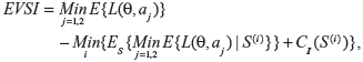
If we know the cost of collecting each additional sample datum, then the expected net gain of sampling information (ENGS) can be derived. The sample size with the highest ENGS will be the optimum.25 Figure 2 shows the relationships among EVSI, CI, and ENGS.
 | Figure 2 Relationships among EVSI, CI, and ENGS. |
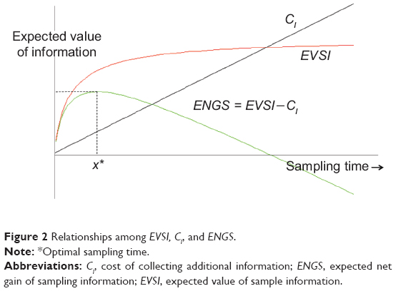
We also assume that the same rate of decrease in the variance can also be used to study the value of imperfect information in the case of trends. Figure 3 shows the expected value of imperfect information about λ0, when λ0 has a gamma prior distribution for the power law failure model. Since the value of imperfect information gets larger as the sampling time gets longer, we can then determine the optimal sampling time based on the assumption that the cost of collecting additional information is linear in the sampling time x. Empirical investigation suggests that collecting additional information tends to be worthwhile for short sampling times, but that the gain from collecting additional information eventually decreases as the sampling time gets longer.
 | Figure 3 Expected value of imperfect information about λ0. |
Quantitative information analysis
Quantitative information here is considered to be sample information that comes from an actual clinical dataset. Suppose that a patient has a planned lifetime T, and the decision of whether to maintain the status quo or to perform some intervention treatment at time t must be made, the decision variable we are dealing with is then the expected number of failures during the time period [t,T]. Since failure times are assumed to be drawn from an NHPP with the intensity function λ(t)=λ0h(β;t), the expected number of failures in [t,T] under the status quo is given by:
|
|
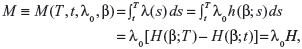
where 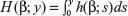 , and H=H(β)=H(β;T)−H(β;t). Suppose that undertaking the intervention treatment will reduce the failure intensity by a fraction ρ, where 0<ρ<1. Then, the expected number of failures in [t,T], if the intervention treatment is performed, is given by:
| (4) |

On the basis of the assumptions given above, we therefore have a two-action problem with a linear loss function, where the loss for taking action a1 (ie, continuing with the status quo) is CAM and the loss for taking action a2 (ie, undertaking the intervention treatment) is CA(1−ρ)M+CR, where CA is the cost of a failure if it occurs, and CR is the cost of the proposed undertaking of the intervention treatment. The expected loss for the status quo is simply CAE{M}, and the expected loss for undertaking the intervention treatment is CA(1−ρ)E{M}+CR. If we substitute in the functional form for H corresponding to a particular failure model, we can then perform a Bayesian decision analysis. Since we have a two-action problem with linear loss, it is apparent that the expected value of perfect information (EVPI) is:
|
|
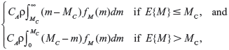
where MC=CR/(CAρ) is the cutoff value of E{M} for undertaking the intervention treatment.
In this case, it is relatively easy to identify the optimal decision,26 since the NHPP data can be transformed to equivalent homogeneous Poisson process data by the transformation z=H(β;x).
The linear failure model
The likelihood functions have a common kernel function of the form  , where
 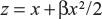 for the linear failure model. Bayesian prior and posterior analyses can be carried out simply by comparing the mean values of λ0 with the cutoff value τC for prior and posterior analysis.6 If the mean values of prior and posterior are smaller than τC, then we should maintain the status quo; if not, then we should undertake the intervention treatment. The values of τC for the linear failure model can be derived as follows:
| (6) |
The power law failure model
The likelihood functions have a common kernel function of the form  , where z=xβ in the power law failure model. Bayesian prior and posterior analyses can be carried out simply by comparing the mean values of λ0 with the cutoff value τC for prior and posterior analysis.11 If the mean values of prior and posterior are smaller than τC, then we should maintain the status quo; if not, then we should undertake the intervention treatment. The values of τC for the power law failure model can be derived as follows:
| (7) |
The exponential failure model
The likelihood functions have a common kernel function of the form  , where z=[exp(βx)−1]/β for the exponential failure model. Bayesian prior and posterior analyses can be carried out simply by comparing the mean values of λ0 with the cutoff value τC for prior and posterior analysis.5 If the mean values of prior and posterior are smaller than τC, then we should maintain the status quo; if not, then we should undertake the intervention treatment. The values of τC for the exponential failure model can be derived as follows:
| (8) |
Suppose λ0 is distributed as Gamma(m,y). The posterior distribution for λ0 will then be Gamma(m+n,y+z). In this case, the EVSI is given by
|
|
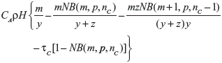
when E{λ0} ≤ τC, and by
|
|
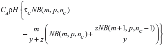
when E{λ0}>τC, where NB(a,b,c) denotes the cumulative distribution function of the negative binomial distribution with parameters a and b evaluated at point c, nC is the smallest integer greater than or equal to τC(y+z)−m, and p=y/(y+z).
The case of known λ0 and unknown β
As with the initial failure rate λ0, the information we collect for β may be imperfect. Detailed root cause analysis could conceivably provide information only about β; for example, by revealing whether the root causes of observed failures were related to the process of aging.
Qualitative information
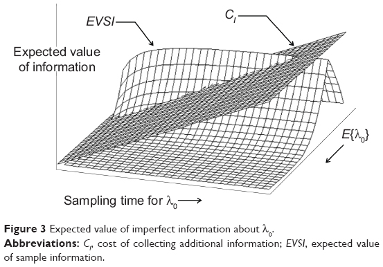
In analyzing qualitative information, we make the same heuristic assumptions as qualitative information analysis and apply the same assumed rate of decrease in the variance of β. Figure 4 shows the expected value of imperfect information when β has a uniform prior distribution for the power law failure model. Since the value of imperfect information gets larger as the sampling time gets longer, we can then determine the optimal sampling time based on the assumption that the cost of collecting additional information is linear in the sampling time. Empirical investigation suggests that collecting additional information tends to be worthwhile for short sampling times, but that the gain from collecting additional information (CI) eventually decreases as the sampling time gets longer.
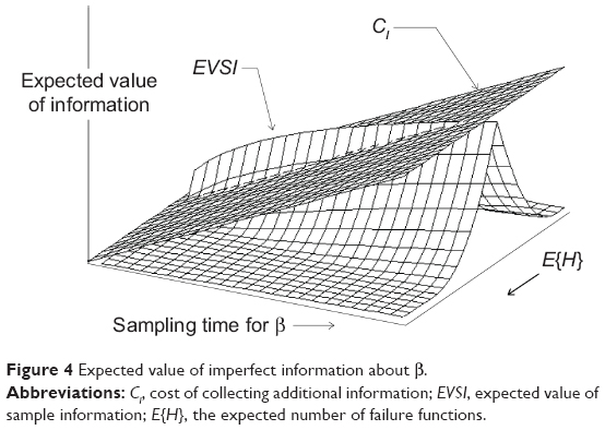 | Figure 4 Expected value of imperfect information about β. |
Quantitative information analysis
The EVSI and the ENGS are not available when the sample information is from actual clinical failure data. Physicians can judge whether collecting additional information from clinical data is worthwhile only by referring to the expected value of perfect information (eg, according to the EVPI, the physician can evaluate whether collecting additional information from clinical data is worthwhile or not). Bayesian prior and posterior analysis can be carried out as long as the prior and posterior expectations for H can be obtained, either analytically or numerically. Based on the results of Chang et al12 we can compare the prior and/or posterior mean values of H with the cutoff value τC. If the relevant mean is smaller than τC, then we should maintain the status quo; if not, then we should undertake the intervention treatment.
The case of unknown λ0 and unknown β
As with, the information we collect for both λ0 and β may be imperfect.
Qualitative information
If both λ0 and β are qualitative, we can make the same heuristic assumptions and apply the known rates of decrease in the variances of λ0 and β, respectively. Figure 5 shows the expected value of imperfect information about λ0 and β when λ0 has a gamma prior distribution and β has a uniform prior distribution for the power law failure model. Since the value of imperfect information gets larger as the sampling time gets longer, we can determine the optimal sampling time based on the assumption that the cost of collecting additional information is linear in the sampling time. Empirical investigation suggests that collecting additional information tends to be worthwhile for short sampling times, but that the gain from collecting additional information eventually decreases as the sampling time gets longer.
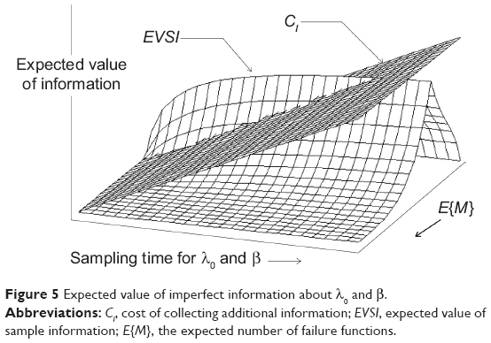 | Figure 5 Expected value of imperfect information about λ0 and β. |
Quantitative information
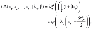
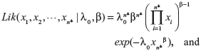
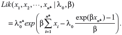
When actual clinical failure data are available, neither the EVSI nor the ENGS information are available. However, prior and posterior analyses can be performed as long as the prior and posterior expectations for M (ie, the expected number of recurrent events under the status quo) can be derived, either analytically or numerically. The likelihood functions of the first n* failure times for the linear, power law, and exponential failure models are, respectively:
|
|
|
|
|
|
The joint posterior distribution for λ0 and β obtained by Bayesian updating is simply proportional to the product of the joint prior distribution for λ0 and β and the likelihood function. However, the derivation of the posterior analysis is often cumbersome and must generally be performed by numerical integration. Furthermore, if the prior distributions for λ0 and β are Gamma(α,γ) and Uniform(a,b), respectively, then the joint posterior distribution for λ0 and β, which the given likelihood function can be obtained by incorporating equation (11), (12) and (13) as the following:
|
|
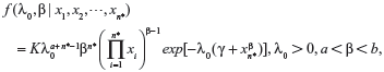
where 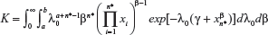 is the normalizing constant.
Once the posterior joint distributions for λ0 and β are obtained, the posterior density function for M (ie, the expected number of failures during the time period [t,T] under the status quo) can be derived by substituting the appropriate densities for λ0 and β. Bayesian prior and posterior analyses can be carried out by comparing the prior and posterior mean values of M with the cutoff value MC. If the relevant mean is smaller than MC, then we should maintain the status quo; if not, then we should undertake the intervention treatment.
Example with recurrent chronic granulomatous disease
In order to analyze the behavior of the proposed model, a set of recurrence events data were simulated with chronic granulomatous disease (CGD).1 CGD is an inherited disease caused by defects in superoxide-generating nicotinamide adenine dinucleotide phosphate (NADPH). Most cases of CGD are transmitted as a mutation on the X chromosome and can also be transmitted via CYBA and NCF1 and affect other PHOX proteins. In developed countries, survival of CGD patients have lived beyond the third decade of life. In developing countries, both delay in diagnosis of CGD and poor compliance with long-term antimicrobial prophylaxis are responsible for high morbidity and premature mortality. In one study, the use of prophylactic itraconazole reduced the incidence of fungal infections, but the effectiveness of long-term prophylaxis remains to be evaluated. Patients with CGD benefit from recombinant human interferon-γ (rIFN-γ) prophylaxis. However, fungal infections remain the main cause of mortality in CGD. Failure data from a trial of immunotherapy for the treatment of CGD have been previously studied.27 In this study, we have used the unknown λ0 and known β case to illustrate the model developed in preposterior analysis. We assume that the cost of collecting and analyzing actual failure data is US$500 per year from the start of the observation period t0=4.417. The assumption of US$500 per year for collecting actual clinical failure data is made to give the same cost as in the case of perfect information (ie, CI=10,000) if the data are collected for the entire 20 years. The optimal sampling time can then be evaluated. In this example, since the clinical failure data are already available, we assume that the cost of analyzing the clinical failure data is associated with tasks such as reviewing medical records and interviewing physicians. Discounting of the data collection cost over time is not considered.
The purpose of this study was to identify the ranges of numerical values for which each option will be most efficient with respect to the input parameters. If the recurrent process of CGD is modeled by the linear failure model with β=0.6, then the optimal sampling time is 11.300 years from the start of the observation period. The ENGS for this case is 8,595.52. If the recurrent process of CGD is modeled by the power law failure model with β=1.65, then the optimal sampling time is 10.277 years from the start of the observation period. The ENGS for this case is 6,410.37. If the recurrent process of CGD is modeled by the exponential failure model with β=0.16, then the optimal sampling time is 14.541 years from the start of the observation period. The ENGS for this case is 10,117.91. Since the optimal sampling period of [4.317,14.541] exceeds the observation period of [4.317,14.417], we would presumably use the entire available dataset. In this case, the ENGS would be 10,034.40, which is slightly smaller than the net gain of 10,117.91 that would be expected if data from the full 10.224 years identified as optimal were available. The above results are consistent with the results of EVPI, which show that collecting perfect information would be desirable for all three clinical failure models (and hence that collecting imperfect information might also be worthwhile).
Prior and posterior analyses
Prior and posterior analyses can be carried out by comparing the prior and posterior mean values of λ0 with the cutoff value τC. If the mean of λ0 is smaller than τC, then we should maintain the status quo; if not, then we should undertake the intervention.
Linear failure model
If the recurrent process of CGD is modeled by the linear failure model with β=0.6, then the cutoff value of E{λ0} at which the risk reduction action becomes cost-effective is τC=CR/{CAρ[T−t+β(T2−t2)/2]}=0.1186. Since the prior mean E{λ0}=0.1 is smaller than τC, maintaining the status quo would be the optimal prior decision (ie, prior to collecting any information). Taking into account the failure data within the optimal sampling period [4.317,11.300], the posterior mean E′{λ0} is 0.2090, which is greater than τC, so undertaking the risk reduction action would be the optimal posterior decision.
Power law failure model
If the recurrent process of CGD is modeled by the power law failure model with β=1.65, then the cutoff value of E{λ0} at which the risk reduction action becomes cost-effective is τC=CR/{CAρ(Tβ−tβ)}=0.1282. Since the prior mean E{λ0}=0.1 is smaller than τC, maintaining the status quo would be the optimal prior decision. Taking into account the failure data within the optimal sampling period [4.317, 10.277], the posterior mean E′{λ0} is 0.1673, which is greater than τC, so undertaking the risk reduction action would be the optimal posterior decision.
Exponential failure model
If the recurrent process of CGD is modeled by the exponential failure model with β=0.16, then the cutoff value of E{λ0} at which the risk reduction action becomes cost-effective is τC=CR/{CAρ[exp(βT)−exp(βt)]/β}=0.08281. Since the prior mean E{λ0}=0.1 is greater than τC, undertaking the risk reduction action would be the optimal prior decision. Taking into account the failure data within the total available observation period [4.317,14.417], the posterior mean E′{λ0} is 0.1906, which is still greater than τC, so undertaking the risk reduction action would also be the optimal posterior decision.
Table 1 summarizes the results of the analyses performed for the case of unknown λ0 and known β. As can be seen from Table 1, the observed data generally support the adoption of the risk reduction action. This is also supported by the prior analysis for the exponential failure model (which shows a steep increase in failure rate after the end of the observation period), but not by the prior analysis for the linear and power law failure models (which show much less steep increases).
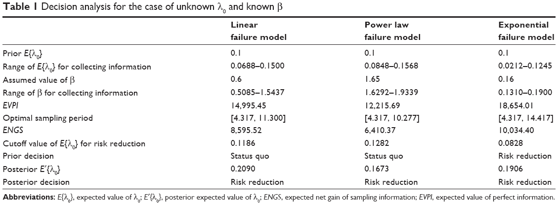 | Table 1 Decision analysis for the case of unknown λ0 and known β |
Discussion
The effective management of uncertainty is one of the most fundamental problems in medical decision-making. Currently, most medical decision models rely on point estimates for input parameters, although the uncertainty surrounding these values is well recognized. It is natural that the physician should be interested in the relationship between changes in those values and subsequent changes in model output.
The empirical investigation of the CGD case study was discussed as follows. First, the base case in the case of unknown λ0 and known β, the width of values of λ0 within which collecting additional information is desirable is larger for the exponential failure model than for either the linear failure model or the power law failure model. Similarly, the EVPI for the base case is larger for the exponential failure model than for the other failure models. These results suggest that the possibility of rapid aging with the exponential failure model may make reduction of uncertainty more important, as one might expect (although it would not have been entirely clear a priori whether we should expect the possibility of rapid aging to favor data collection or the immediate adoption of the risk reduction action).
Second, in the case of known λ0 and unknown β, and the width of the range of values of E{M}, within which collecting additional information is desirable is much larger for both the power law failure model and the exponential failure model than for the linear failure model. This is because the functional form of M is more sensitive to the value of β for the power law and exponential failure models than for the linear failure model. The range of values of λ0 within which collecting additional information is desirable is also larger for the power law and exponential failure models than for the linear failure model. Finally, the EVPI is larger for both the power law and exponential failure models than for the linear failure model. These results again show the importance of reducing uncertainty when rapid aging is possible, as is intuitively reasonable. Similar results are also found in the case of unknown λ0 and unknown β.
Overall, as one could expect, the case of unknown λ0 and unknown β represents greater uncertainty than the other two cases, since the EVPI for the case of unknown λ0 and unknown β is larger than for the other two cases. Thus, even with the linear failure model (where the prior decision is always to maintain the status quo), the optimal posterior decision is to undertake the risk reduction action. In this study, an NHPP was used for describing the CGD. Three kinds of failure models (linear, exponential, and power law) were considered, and the effects of the scale factor and the aging rate of these models were investigated. The failure models were studied under the assumptions of unknown scale factor and known aging rate, known scale factor and unknown aging rate, and unknown scale factor and unknown aging rate, respectively. In addition, in order to analyze the value of information under imperfect, we devised a method for experts’ knowledge which are usually the absence of sharply defined criteria for dealing with such situations. Further, we demonstrated our method with an analysis of data from a trial of immunotherapy in the treatment of CGD. In some situations, the data were simply inadequate for any predictions to be made with a high level of confidence. Thus, it is recognized that practical judgments are very often, inevitably, strongly guided by subjective judgment. Bayesian decision analysis provides a means of quantifying subjective judgments and combining them in a rigorous way with information obtained from experimental data. Instead of considering only the sparse failure data, Bayesian analysis can provide a technique by which prior knowledge, such as expert opinion, past experience, or similar situations, can be taken into account.
Conclusion
The scientific development on clinical decision-making is toward a model-based analysis with evidence of available data. The diverse clinical data and events make complicated clinical decision-making an actual evaluating challenge. One approach to this issue is to develop a Bayesian information-value analysis that explicitly represents that the history of the disease along with concomitant variables and the impact of treatments. The Bayesian decision model is essential by which the impact of alternative clinical scenarios and uncertainty in model input can be evaluated. The Bayesian decision analysis can be useful for determining, analytically or numerically, the conditions under which it will be worthwhile to collect additional information. Value-of-information analysis can provide a measure of the expected payoff from proposed research, which can be used to set priorities in research and development. In addition, it seems reasonable to assume that the information we collect will be imperfect. In such situations, it becomes important to choose the optimal sampling time or the optimal sample size. Since more extensive sampling will give us information that is more nearly perfect, but only at an increased cost, knowing the value of information is a good basis for determining the optimal amount of information to collect. In this study, a major concern was on how the imperfect information value should be interpreted, integrated, simulated, and effectively linked to medical practice. Three clinical failure models (the linear, power law, and exponential failure models) were evaluated to give a better understanding of the differing history of the disease associated with concomitant variables. Based on the results of this study, the power law and exponential failure models appear to be more sensitive than the linear failure model toward the requirement of being requisite among others. In particular, the result of exponential failure model may be less realistic, since the intensity function often becomes too steep after the observation period. One area in which further work might be desirable is in the study of other failure models using the same procedure developed in this study.
Acknowledgments
The authors wish to express their sincere thanks to Professor Shaw Wang for the helpful English language copy editing and to the reviewers for comments on an early draft of this paper. This work is supported by the Jen-Ai Hospital and Chung-Shan Medical University of Taiwan (CSMU-JAH-103-01).
Disclosure
The authors report no conflicts of interest in this work.
References
Cook RJ, Lawless JF. The Statistical Analysis of Recurrent Events. New York, NY: Springer; 2007. | ||
Kelly PJ, Lim LL. Survival analysis for recurrent event data: an application to childhood infectious diseases. Stat Med. 2000;19(1):13–33. | ||
Tseng CJ, Lu CJ, Chang CC, Chen GD. Application of machine learning to predict the recurrence-proneness for cervical cancer. Neural Comput Appl. 2014;24(6):1311–1316. | ||
Belot A, Rondeau V, Remontet L, Giorgi R; CENSUR working survival group. A joint frailty model to estimate the recurrence process and the disease-specific mortality process without needing the cause of death. Stat Med. 2014;33(18):3147–3166. | ||
Chang CC, Ting WC, Teng T, Hsu CH. Evaluating the accuracy of ensemble learning approaches for prediction on recurrent colorectal cancer. International Journal of Engineering and Innovative Technology. 2014;3(10):19–22. | ||
Schneider S, Schmidli H, Friede T. Blinded sample size re-estimation for recurrent event data with time trends. Stat Med. 2013;32(30):5448–5457. | ||
Cox DR, Lewis PAW. The Statistical Analysis of Series of Events. London: Chapman and Hall; 1966. | ||
Qin R, Nembhard DA. Demand modeling of stochastic product diffusion over the life cycle. International Journal of Production Economics. 2012;137(2):201–210. | ||
Speybroeck N, Praet N, Claes F, et al. True versus apparent malaria infection prevalence: the contribution of a Bayesian approach. PLoS One. 2011;6(2):e16705. | ||
Gustafson P. The utility of prior information and stratification for parameter estimation with two screening tests but no gold standard. Stat Med. 2005;24(8):1203–1217. | ||
Chang CC, Cheng CS, Huang YS. A web-based decision support systems for chronic diseases. J Univers Comput Sci. 2006;12(1):115–125. | ||
Pratt J, Raiffa H, Schlaifer R. Introduction to Statistical Decision Theory. Cambridge, MA: Massachusetts Institute of Technology (MIT); 1995. | ||
Wendt D. Value of information for decisions. J Math Psychol. 1969;6:430–443. | ||
Chang CC, Cheng CS. A structural design of clinical decision support system for chronic diseases risk management. Cent Eur J Med. 2007; 2(2):129–139. | ||
Menten J, Boelaert M, Lesaffre E. Bayesian meta-analysis of diagnostic tests allowing for imperfect reference standards. Stat Med. 2013; 32(30):5398–5413. | ||
Willan AR, Simon E. Optimal clinical trial design using value of information methods with imperfect implementation. Health Econ. 2010; 19(5):549–561. | ||
Gething PW, Noor AM, Goodman CA, et al. Information for decision making from imperfect national data: tracking major changes in health care use in Kenya using geostatistics. BMC Med. 2007;5:37. | ||
Albert PS. Estimating diagnostic accuracy of multiple binary tests with an imperfect reference standard. Stat Med. 2009;28(5):780–797. | ||
Bertens LCM, Broekhuizen BDL, Naaktgeboren CA, et al. Use of expert panels to define the reference standard in diagnostic research: a systematic review of published methods and reporting. PLoS Med. 2013;10(10):e1001531. | ||
Chang CC. Bayesian value of information analysis with linear, exponential, power law failure models for aging chronic diseases. J Comput Sci Eng. 2008;2(2):201–220. | ||
Azondékon SH, Martel JM. “Value” of additional information in multicriterion analysis under uncertainty. Eur J Oper Res. 1999;117(1):45–62. | ||
Schlaifer R. Probability and Statistics for Business Decisions: An Introduction to Managerial Economics under Uncertainty. New York: McGraw-Hill; 1959. | ||
Raiffa H, Schlaifer R. Applied Statistical Decision Theory. Cambridge, MA: Massachusetts Institute of Technology (MIT) Press; 1968. | ||
Ren D, Stone RA. A Bayesian approach for analyzing a cluster-randomized trial with adjustment for risk misclassification. Comput Stat Data Anal. 2007;51(12):5507–5518. | ||
Dendukuri N, Rahme E, Bélisle P, Joseph L. Bayesian sample size determination for prevalence and diagnostic test studies in the absence of a gold standard test. Biometrics. 2004;60(2):388–397. | ||
Soland RM. Bayesian analysis of the Weibull process with unknown scale parameter and its application to acceptance sampling. IEEE Transactions on Reliability. 1698;R-17(2):84–90. | ||
[No authors listed]. A controlled trial of interferon gamma to prevent infection in chronic granulomatous disease. The International Chronic Granulomatous Disease Cooperative Study Group. N Engl J Med. 1999; 324:509–516. |
 © 2014 The Author(s). This work is published and licensed by Dove Medical Press Limited. The full terms of this license are available at https://www.dovepress.com/terms.php and incorporate the Creative Commons Attribution - Non Commercial (unported, v3.0) License.
By accessing the work you hereby accept the Terms. Non-commercial uses of the work are permitted without any further permission from Dove Medical Press Limited, provided the work is properly attributed. For permission for commercial use of this work, please see paragraphs 4.2 and 5 of our Terms.
© 2014 The Author(s). This work is published and licensed by Dove Medical Press Limited. The full terms of this license are available at https://www.dovepress.com/terms.php and incorporate the Creative Commons Attribution - Non Commercial (unported, v3.0) License.
By accessing the work you hereby accept the Terms. Non-commercial uses of the work are permitted without any further permission from Dove Medical Press Limited, provided the work is properly attributed. For permission for commercial use of this work, please see paragraphs 4.2 and 5 of our Terms.