Automated measurements of human cone photoreceptor density in healthy and degenerative retina by region-based segmentation

Introduction

Adaptive optics scanning laser ophthalmoscope (AOSLO) permits a direct en face view of human cone photoreceptors.¹ The high-resolution en face images obtained using AOSLO have been used to investigate alterations in the photoreceptor densities in eyes with degenerative retinal diseases such as cone-rod dystrophy,^2,3 retinitis pigmentosa (RP),^4,5 acute zonal occult outer retinopathy (AZOOR),⁶ and occult macular dystrophy.⁷ In such degenerative retinal diseases, measurements of cone photoreceptor densities can be used to follow up the progression of the degeneration or the effectiveness of therapy in preserving the photoreceptors.⁵

Automated methods have been used to identify individual cone photoreceptors and determine the density of the cones in healthy eyes.^8–14 In many studies designed to determine cone density, individual cones are identified by automatically detecting bright spots on a cone mosaic image. The cone mosaic images are averaged and filtered using a spatial frequency filtering (SFF) technique to avoid misidentification of the cones because of image noise. The SFF technique is based on the fast Fourier transform (FFT) method. This technique was widely used in earlier studies on the automated calculation of the cone densities in the AOSLO images, and it was based on intensity enhancement and noise reduction, ie, increasing the signal-to-noise ratio. For this technique to be effective, the images must have a periodic structure like the cone mosaic images in healthy eyes. In healthy eyes, the cone mosaic images have a periodical structural pattern, ie, they have a spatial frequency pattern. This information can be used to estimate cone densities. Cooper et al¹⁵ estimated cone density from a power spectrum of cone mosaic images without identification of individual cones. The central issue in the clinical use of an automated measurement of cone densities is its ability to obtain accurate values. Accuracy is important in determining whether the cone densities are significantly different from normal densities and whether they have changed significantly over time or after therapy. Recently, several studies evaluated the accuracy and stability of determining cone photoreceptor density manually or by an automated identification method.^16,17 In these studies, healthy cone mosaic images were photographed by AOSLO repeatedly in the same retinal location, and the accuracy and stability of estimated cone photoreceptor density were evaluated. However, automated estimation methods have been used to assess the effect of some retinal degenerative diseases on cone densities.^18,19 In these studies, cone density was estimated by manual identification or automated identification with manual collection. In fact, fully automated estimation of cone density in degenerated cone mosaic images may include considerable misidentification because of vague structures of the affected tissues. However, manual identification and corrections would be too time-consuming and not appropriate for the clinic. To overcome this deficit, we have developed a technique based on a region-based segmentation algorithm for determining the cone densities. A region-based segmentation algorithm has been commonly applied in image processing studies for various purposes.²⁰ An approach for estimating cone density using a region-based segmentation without spatial filtering has not been reported. The region-based segmentation technique can reduce misidentifications of the cone mosaic images, which have unique features or non-periodic structure, because this technique does not use the spatial frequency information, and it should be particularly effective, especially, in diseased eyes with a non-periodic pattern of the cone mosaic.

The purpose of this study was to estimate cone density by region-based segmentation for cone mosaic images. We estimated the cone densities automatically, both healthy and degenerative cone mosaic images, using our methods. We compared our method with a conventional SFF method and manual identification to examine the possibility of the clinical application of automated cone density counting.

Subjects and methods

Subjects

A total of 15 eyes of 15 healthy subjects consisting of eight men and seven women were studied. None of these subjects had any ocular pathology. The mean axial length was 25.20±1.67 mm with a range of 23.11–27.22 mm. We also examined a man with macular dystrophy (subject 16), a woman with RP (subject 17), and a woman with AZOOR (subject 18). The patients were diagnosed at the Department of Ophthalmology, Osaka University School of Medicine. This research protocol was approved by the institutional review board of the Osaka University Medical School, and the procedures used conform to the tenets of the Declaration of Helsinki. All subjects provided written informed consent.

AOSLO imaging

Details of the custom-built AOSLO (Topcon Corporation, Tokyo, Japan) used in this study have been published.²¹ The AOSLO images were taken through dilated pupils, and the ciliary muscle was paralyzed by topical tropicamide (0.5%) and phenylephrine (0.5%) in all subjects. The AOSLO system can take 400 sequential images at a rate of 30 frames/s, and the retinal image can be displayed in real-time. The field of view (FOV) can be immediately varied from 0.20°×0.23° to 6.4°×7.2°. All the cone mosaic images were obtained with a 0.8°×0.9° field. In addition, retinal images were also obtained with a 3.2°×3.6° field to construct montage images and determine the foveal center (Figure 1). The montage images were used to verify the location of the high-magnification cone mosaic images. The subjects were instructed to fixate on a target displayed on a built-in organic electro luminescent diode display, which could be moved to obtain photographs of different retinal sites. We determined foveal center with wide FOV images. First, the retinal image was acquired with a wide FOV mode as 6.4°×7.2° or 3.2°×3.6°, and the subject was instructed to fixate a built-in target display. Then, to determine the position of the target corresponding to the foveal center, the target was moved to almost align the center of the FOV with the foveal center. To evaluate our algorithm for measuring parafoveal cone photoreceptor density at different retinal locations, cone mosaic images were photographed at 0.5, 1.0, and 1.5 mm temporal to the center of the fovea. The fixiation target was moved to previously calculated coordinate that corresponds to each retinal eccentricity. The angular coordinates of the fixation target are indicated in degrees. To convert the angle to the linear scale, we calculated the retinal magnification factor (RMF) from the axial length of each subject.^22,23 The RMF is a factor that represents conversion from angle to linear scale on the retina (mm/degree). The RMF can be calculated from the axial length x as RMF =0.01306·(x −1.82). For instance, the linear distance on retina t can be calculated using the RMF and the angle of incident ray U in degrees as t = RMF·U.²³

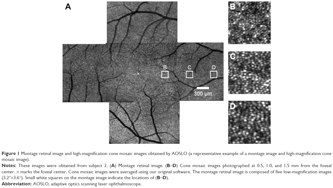Figure 1 Montage retinal image and high-magnification cone mosaic images obtained by AOSLO (a representative example of a montage image and high-magnification cone mosaic image). Notes: These images were obtained from subject 2. (A) Montage retinal image. (B–D) Cone mosaic images photographed at 0.5, 1.0, and 1.5 mm from the foveal center. × marks the foveal center. Cone mosaic images were averaged using our original software. The montage retinal image is composed of five low-magnification images (3.2°×3.6°). Small white squares on the montage image indicate the locations of (B–D). Abbreviation: AOSLO, adaptive optics scanning laser ophthalmoscope.

The axial length was measured using an optical biometer (AL-Scan; Nidek Co., Aichi, Japan). A fixation point of the angular coordinates in degrees corresponding to 0.5, 1.0, and 1.5 mm temporal to the center of the fovea was calculated from the RMF.

For one trial, ~400 sequential images were obtained at 30 frames/s. In the 15 healthy subjects, we recorded 10 trials with a short break between each of the three locations on the retina. Cone mosaic image sequences were obtained for a total of 30 trials for each subject to calculate the cone photoreceptor density in each trial using the software we developed with the three different methods, as described later. However, only one trial was obtained in the three patients with retinal degeneration because many repeated trials could be a burden to the patients. For all patients, a high- and low-magnification-affected retinal image ~1.0 mm temporal to the fovea was obtained. We selected and generated five averaged images from 400 sequential images included in one trial. Then, a total of 15 averaged degenerative cone mosaic images from three patients were generated. We also calculated cone density of diseased cone mosaic images using three methods under the same procedure as the healthy eyes.

Image averaging

The algorithm for analyzing cone density consisted of several image processing steps. To eliminate inappropriate images for averaging, 10 strongly correlated sequential images were automatically selected from the 400 sequential images taken at one time. These selected images were averaged to increase the signal-to-noise ratio for subsequent analysis. The selected sequential images were similar to each other, but they were misaligned because of microsaccades. To obtain an averaged image, all misaligned sequential images were superposed as accurately as possible. Our technique uses several steps to superpose sequential images. The images were matched from relatively large to relatively small areas, step-by-step, for accurate superpositioning. Finally, the superposed images were averaged pixel by pixel except for the pixels that had values markedly different from those in the other images. All averaged images were cropped to 256×256 pixels. The cone photoreceptor density was calculated from the number of individual cone cells in the cropped area of the averaged images. The number of individual cone cells was counted with our automated algorithm based on the region-based segmentation technique. We also counted the number of cells in the same cropped area with the conventional SFF method and the manual identification method (MIM). Finally, the cone densities were converted to cells/mm². The cropped window area of an image (256×256 pixels) corresponded to ~0.41°×0.33° on the scan angle of our AOSLO. This window area is approximately equivalent to 120×100 μm at 24 mm axial length, which is enough to estimate cone densities.²⁴ The square image area is not equivalent to the square area on the retina because of the correction for the distortion of the raw digital image. The scan angle was converted to a retinal distance in millimeter using the RMF of each subject. Then, the square area of the analyzed retinal area was calculated in square millimeter. The cone photoreceptor density was calculated from the number of individual cone photoreceptor cells and the square measure of the analyzed retinal area.

Region-based segmentation method (RSM)

The region-based segmentation technique was used to identify individual cones without any spatial filtering. Our algorithm has four steps that are illustrated in Figure 2. To estimate cone density, the number of divided segments is counted instead of detecting by peak bright spot. First, the averaged cone mosaic image is enhanced with a morphological dilation process to prevent misidentification of cone cells that have relatively lower brightness than the surrounding cells. Then, the binarization was applied to the enhanced image. To avoid the effects of regional differences in brightness, the image was binarized by adaptive thresholding of Otsu’s method.²⁵ After binarization, the contours of the cone cells were segmented. To eliminate pixel noise, segments with a smaller size than the predetermined threshold were deleted. The appropriate threshold was empirically determined for the best retinal image at each retinal location. The threshold on each retinal location was fixed for all healthy subjects. Finally, the cone density was calculated from the number of segmented cone cells in the analysis window of the cone mosaic image.

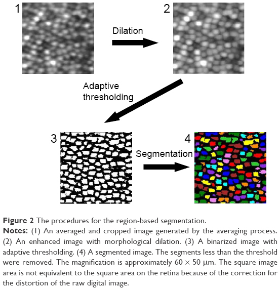Figure 2 The procedures for the region-based segmentation. Notes: (1) An averaged and cropped image generated by the averaging process. (2) An enhanced image with morphological dilation. (3) A binarized image with adaptive thresholding. (4) A segmented image. The segments less than the threshold were removed. The magnification is approximately 60 × 50 mm. The square image area is not equivalent to the square area on the retina because of the correction for the distortion of the raw digital image.

SFF method

We also estimated the cone density by the SFF method, which is similar to previous studies with AOSLO.⁹ The procedures for spatial filtering method (SFM) are shown in Figure 3. The averaged image was converted to a frequency domain image by FFT. Then, the spatial frequency band-pass filter was applied to the frequency domain image. The filtered frequency domain image was converted to a spatial domain image by inverse FFT. Finally, the individual cone photoreceptor cells were identified by searching for peak brightness values on the spatial domain image. We determined the appropriate bandwidth of the spatial frequency band-pass filter earlier by experimenting on each retinal location and fixed the bandwidth for all healthy subjects.

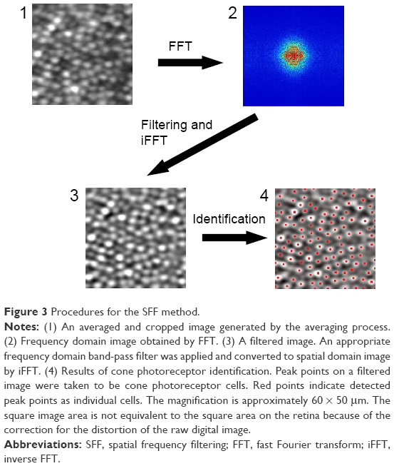Figure 3 Procedures for the SFF method. Notes: (1) An averaged and cropped image generated by the averaging process. (2) Frequency domain image obtained by FFT. (3) A filtered image. An appropriate frequency domain band-pass filter was applied and converted to spatial domain image by iFFT. (4) Results of cone photoreceptor identification. Peak points on a filtered image were taken to be cone photoreceptor cells. Red points indicate detected peak points as individual cells. The magnification is approximately 60 × 50 mm. The square image area is not equivalent to the square area on the retina because of the correction for the distortion of the raw digital image. Abbreviations: SFF, spatial frequency filtering; FFT, fast Fourier transform; iFFT, inverse FFT.

MIM

In previous studies, the MIM or correction in cone counting has been adopted as the benchmark for automatic identification methods.^16,17 We also calculated the cone densities with manual identification of the cone cells in the same image. We manually identified the individual cones and counted the number of cells in the same cone mosaic image. We did this independently before running RSM and SFM.

Statistical data analyses

We compared the results from RSM and SFM with MIM to evaluate the accuracy of the cone density calculated by our method. The cone photoreceptor density derived from MIM on the same retinal cone mosaic images was used as the basis for the accuracy of the automated calculated cone density. The results of the cone density calculated by these three methods were compared in each healthy subject. We evaluated the differences between RSM and MIM and between SFM and MIM using the Wilcoxon rank sum test. A P-value of <0.05 was considered to be statistically significant. We also analyzed the degree of agreement between each method using Bland–Altman plots.²⁶ All data were analyzed using SigmaPlot 12.0 (Systat Software San Jose, CA) and R (R core team, Vienna, Austria).

Results

We calculated the cone density at retinal eccentricities of 0.5, 1.0, and 1.5 mm from the center of the fovea by the two automated methods and the MIM. The average ± standard deviation (SD) of the cone densities, which were sequentially photographed 10 times on 15 normal subjects, is shown in Table 1 and Figure 4.

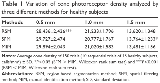Table 1 Variation of cone photoreceptor density analyzed by three different methods for healthy subjects Notes: Average cone density of 150 trials (10 sequential trials of 15 healthy subjects, cells/mm2) ± SD. *P<0.05 (SFM > MIM, Wilcoxon rank sum test) and ***P<0.001 (RSM < MIM, Wilcoxon rank sum test). Abbreviations: RSM, region-based segmentation method; SFM, spatial filtering method; MIM, manual identification method; SD, standard deviation.

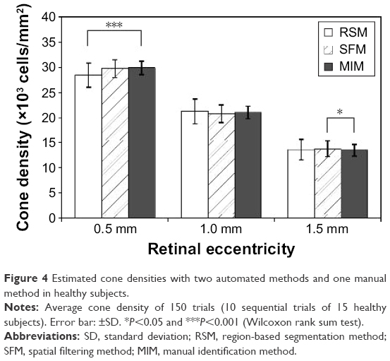Figure 4 Estimated cone densities with two automated methods and one manual method in healthy subjects. Notes: Average cone density of 150 trials (10 sequential trials of 15 healthy subjects). Error bar: ±SD. *P<0.05 and ***P<0.001 (Wilcoxon rank sum test). Abbreviations: SD, standard deviation; RSM, region-based segmentation method; SFM, spatial filtering method; MIM, manual identification method.

We found statistically significant differences in the calculated cone densities between RSM and MIM at 0.5 mm retinal eccentricity and between SFM and MIM at 1.5 mm retinal eccentricity. Bland–Altman plots between RSM and MIM and between SFM and MIM are shown in Figure 5. The Bland–Altman plots were made for all trials and healthy subjects at each retinal eccentricity. We found that there were no systematic errors. However, there was a slightly biased error between automated methods and MIM.

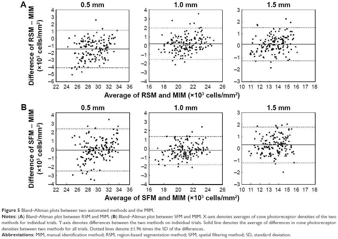Figure 5 Bland–Altman plots between two automated methods and the MIM. Notes: (A) Bland–Altman plot between RSM and MIM. (B) Bland–Altman plot between SFM and MIM. X-axis denotes averages of cone photoreceptor densities of the two methods for individual trials. Y-axis denotes differences between the two methods on individual trials. Solid line denotes the average of differences in cone photoreceptor densities between two methods for all trials. Dotted lines denote ±1.96 times the SD of the differences. Abbreviations: MIM, manual identification method; RSM, region-based segmentation method; SFM, spatial filtering method; SD, standard deviation.

The representative diseased retinal images from each patient are shown in Figure 6A–F. The results of the estimated cone density difference between RSM and MIM and between SFM and MIM of the 15 diseased retinal areas of three patients (five images from each patient) are shown in Figure 7.

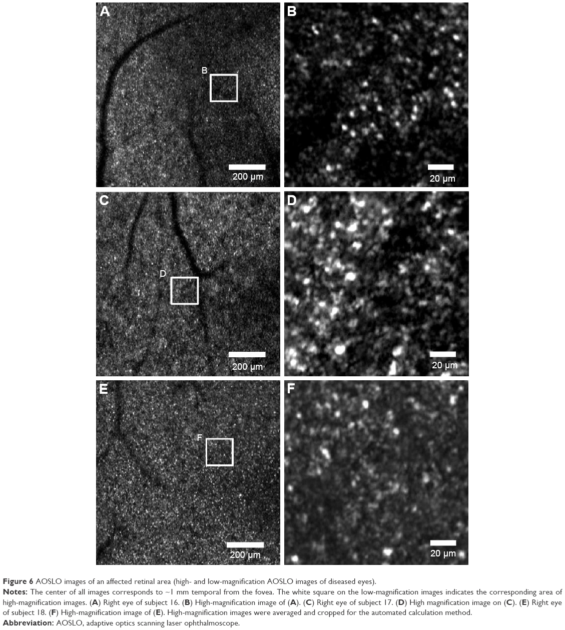Figure 6 AOSLO images of an affected retinal area (high- and low-magnification AOSLO images of diseased eyes). Notes: The center of all images corresponds to ~1 mm temporal from the fovea. The white square on the low-magnification images indicates the corresponding area of high-magnification images. (A) Right eye of subject 16. (B) High-magnification image of (A). (C) Right eye of subject 17. (D) High magnification image on (C). (E) Right eye of subject 18. (F) High-magnification image of (E). High-magnification images were averaged and cropped for the automated calculation method. Abbreviation: AOSLO, adaptive optics scanning laser ophthalmoscope.

Figure 7 Differences in estimated cone densities between automated methods and manual identification of diseased eyes. Notes: A total of 15 diseased retinal areas (five image areas from three patients) were analyzed. RSM-MIM and SFM-MIM denote differences in estimated cone densities between RSM and MIM and between SFM and MIM, respectively. Error bars indicate SD. ***P<0.001 (Wilcoxon rank sum test). Abbreviations: RSM, region-based segmentation method; MIM, manual identification method; SFM, spatial filtering method; SD, standard deviation.

In eyes with retinal degeneration, the cone densities measured by manual estimation were significantly closer to RSM than SFM, with the appropriate threshold levels or the spatial frequency bandwidth. The most appropriate threshold level or the spatial frequency bandwidth was manually determined by way of experimentation of the individual cases. In cases analyzed by RSM and SFM, individual cones were not detected appropriately with the same threshold level or the same spatial frequency bandwidth that was applied in healthy eyes.

Discussion

The densities of human cones have been investigated using the images obtained by AOSLO or in vitro studies. Curcio et al²⁷ measured the human cone and rod densities in whole mounted human retinas, and many recent studies have reported on human cone densities in the fovea using adaptive optics (AO) images.^{10,14,18,28,29} We estimated mean cone densities using RSM at 0.5, 1.0, and 1.5 mm temporal from the fovea to be 28,436, 21,233, and 13,620 cells/mm², respectively, which are the mean values of all trials of all healthy subjects. The estimated cone densities from previous studies and this study are shown in Table 2. The average cone densities of all healthy subjects obtained in our study were consistent with those reported earlier. The slight difference at 0.5 mm of retinal eccentricity was probably caused by slight misjudgment of retinal eccentricity from the foveal center. In fact, a slight difference in retinal point can cause a considerable difference in the cone density near the foveal center. In some studies, the cone density varied with the axial length and age.²⁸ However, the sex and race of the subjects should not affect the cone densities.^10,30

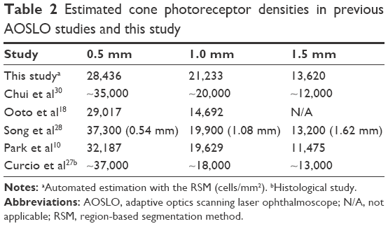Table 2 Estimated cone photoreceptor densities in previous AOSLO studies and this study Notes: aAutomated estimation with the RSM (cells/mm2). bHistological study. Abbreviations: AOSLO, adaptive optics scanning laser ophthalmoscope; N/A, not applicable; RSM, region-based segmentation method.

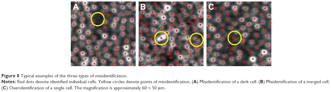
We compared the estimated cone densities between RSM and MIM and between SFM and MIM for each subject with 10 repeated trials. We found statistical significance for the difference between RSM and MIM at 0.5 mm and between SFM and MIM at 1.5 mm (Figure 4). These errors in the automated methods were caused by misidentification of merged cells, dark cells, residual pixel noise, and ambiguous tissues. The merged cells were two or more adjacent cells that were merged and identified as one cell. The average cone density at 0.5 mm retinal eccentricity by RSM was less than that by MIM because of less identification derived from misidentification of merged cells. Merged cells can be separated by spatial band-pass filtering in SFM, and the estimated cone photoreceptor density was closer to the MIM. However, misidentification of merged cells by RSM is considered possible to avoid using features of outline or shape of segments.

The very dark gap regions between cone photoreceptor cells that have low reflectance should cause overidentification because of the residual pixel noise or ambiguous tissues that are not cone photoreceptor cells. In fact, the gap region of cone photoreceptor cells is larger in the outer retinal area than in the inner area. This gap includes rod cells, but it is difficult to resolve distinctly. At 1.5 mm retinal eccentricity, the estimated cone density using SFM was more than that using MIM, which was caused by the overidentification counted at the gap region. These results suggest that in SFM, the SFF may not be suitable to enhance the signals or to suppress noise for non-periodical structures.

Typical example images of these types of misidentifications are shown in Figure 8. The misidentification of merged cells tends to occur in high-density cone mosaic images because of the limited resolution of the AOSLO. This overidentification was derived from overdetermination at the gap between cone photoreceptor cells.

Figure 8 Typical examples of the three types of misidentification. Notes: Red dots denote identified individual cells. Yellow circles denote points of misidentification. (A) Misidentification of a dark cell. (B) Misidentification of a merged cell. (C) Overidentification of a single cell. The magnification is approximately 60 × 50 mm.

We also compared the estimated cone densities of all 15 subjects and all trials with the Bland–Altman plots. The Bland–Altman plots between SFM and MIM and between RSM and MIM are shown in Figure 5. There were no systematic errors, and the biased errors were derived from under- or overidentification. The biased errors of RSM and SFM from MIM were 0.6%–5.1% of the estimated cone density. For healthy subjects, results of biased error and measurement error are considered reasonable, even compared to previous studies of repeated cone density estimation for AO retinal images.^14,16,17

In diseased eyes, we picked five affected retinal areas from each patient. The results of the calculated cone density from the three methods are shown in Figure 7. In addition, examples of identification using two automated methods and MIM for a seriously affected retinal area are shown in Figure 9. We determined the most appropriate threshold level or spatial frequency bandwidth by experimenting for the individual cases. However, the cone densities obtained by SFM were always overestimated with any spatial frequency bandwidth. The results of the diseased eyes shown in Figure 7 indicate the smallest values on SFM, with the most appropriate spatial frequency bandwidth. SFM should overestimate the cone density in the non-periodic very dark areas and vague structures of the affected tissues. However, the cone densities obtained by RSM with the most appropriate threshold were obviously closer to MIM than SFM. These results suggest that RSM has the advantage for non-periodic structures of affected cone mosaic images because RSM does not depend on spatial frequency information of the image. In the affected retinal areas, a cone mosaic image has unique features, such as those shown in Figure 6. For example, it has bright spots, very dark areas, non-periodic cone photoreceptors, and vague structure of the affected tissues.

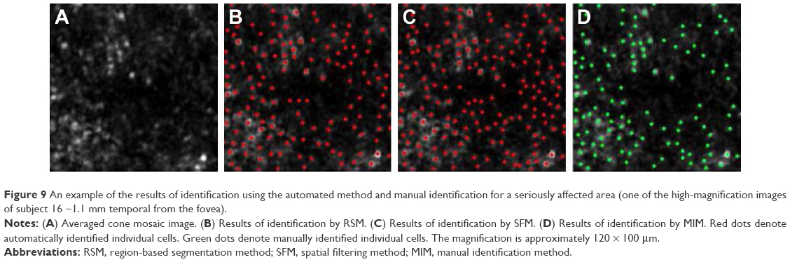Figure 9 An example of the results of identification using the automated method and manual identification for a seriously affected area (one of the high-magnification images of subject 16 ~1.1 mm temporal from the fovea). Notes: (A) Averaged cone mosaic image. (B) Results of identification by RSM. (C) Results of identification by SFM. (D) Results of identification by MIM. Red dots denote automatically identified individual cells. Green dots denote manually identified individual cells. The magnification is approximately 120 × 100 mm. Abbreviations: RSM, region-based segmentation method; SFM, spatial filtering method; MIM, manual identification method.

Even in RSM, an overestimation derived from such patterns could occur, but it can be reduced by applying an appropriate threshold of segment size. RSM rejects smaller bright segments derived from residual pixel noise or affected tissues that were picked up by the threshold of the segment area size. In healthy eyes, the segment size of cone cells can be predicted from previous research results of cone densities. In fact, variations in cone density with retinal eccentricity or axial length were studied in healthy subjects.^22,28 However, the appropriate threshold of RSM must be manually determined before calculating cone density in each case of diseased eyes; this is because of the large variation of cone cell size and affected vague tissues. However, it is considered possible to determine the threshold automatically from some image characteristics of cone mosaic images.

Conclusion

We have developed an automated method for determining the cone densities of human retinas based on a region-based segmentation algorithm in the cone mosaic images photographed by the AOSLO. In healthy subjects, no serious differences were found between the densities determined by our algorithm and the conventional automated algorithm or MIM. The performance of algorithm developed in this work was also demonstrated by the agreement of the measured cone density with the previously published data. In eyes with retinal degeneration, cone density measurement by our method might be more suitable for automated detection compared to the conventional SFF method. The automated cone photoreceptor density estimation can be used in a longitudinal follow-up of disease progression and the effectiveness of therapy in eyes with retinal degeneration. Future studies should focus on the automatic determination of appropriate thresholds and improve accuracy in RSM for various clinical cases in diseased eyes.

Acknowledgments

The authors are thankful to Y Hirohara, M Miwa, and M Saika of Eye Care Technology Development Department, Product Technology Section, Topcon Corporation, for their technical assistance. This work was supported by KAKENHI (25293354) from the Ministry of Education, Culture, Sports, Science and Technology, Japan; Translational Research Network Program from the Ministry of Education, Culture, Sports, Science, and Technology, Japan; and Asian CORE Program from the Japan Society for the Promotion of Science.

Disclosure

The authors report no conflicts of interest in this work.

---

References

1.		Roorda A, Duncan JL. Adaptive optics ophthalmoscopy. Annu Rev Vis Sci. 2015;1:19–50.
2.		Wolfing JI, Chung M, Carroll J, Roorda A, Williams DR. High-resolution retinal imaging of cone-rod dystrophy. Ophthalmology. 2006;113(6):1014–1019.
3.		Choi SS, Doble N, Hardy JL, et al. In vivo imaging of the photoreceptor mosaic in retinal dystrophies and correlations with visual function. Invest Ophthalmol Vis Sci. 2006;47(5):2080–2092.
4.		Duncan JL, Zhang Y, Gandhi J, et al. High-resolution imaging with adaptive optics in patients with inherited retinal degeneration. Invest Ophthalmol Vis Sci. 2007;48(7):3283–3291.
5.		Talcott KE, Ratnam K, Sundquist SM, et al. Longitudinal study of cone photoreceptors during retinal degeneration and in response to ciliary neurotrophic factor treatment. Invest Ophthalmol Vis Sci. 2011;52(5):2219–2226.
6.		Merino D, Duncan JL, Tiruveedhula P, Roorda A. Observation of cone and rod photoreceptors in normal subjects and patients using a new generation adaptive optics scanning laser ophthalmoscope. Biomed Opt Express. 2011;2(8):2189–2201.
7.		Kitaguchi Y, Kusaka S, Yamaguchi T, Mihashi T, Fujikado T. Detection of photoreceptor disruption by adaptive optics fundus imaging and Fourier-domain optical coherence tomography in eyes with occult macular dystrophy. Clin Ophthalmol. 2011;5:345–351.
8.		Li KY, Roorda A. Automated identification of cone photoreceptors in adaptive optics retinal images. J Opt Soc Am A Opt Image Sci Vis. 2007;24(5):1358–1363.
9.		Xue B, Choi SS, Doble N, Werner JS. Photoreceptor counting and montaging of en-face retinal images from an adaptive optics fundus camera. J Opt Soc Am A Opt Image Sci Vis. 2007;24(5):1364–1372.
10.		Park SP, Chung JK, Greenstein V, Tsang SH, Chang S. A study of factors affecting the human cone photoreceptor density measured by adaptive optics scanning laser ophthalmoscope. Exp Eye Res. 2013;108:1–9.
11.		Chitchian S, Boretsky AR, Kuijk FJ, Motamedi M. An edge detection approach for mapping of the human cone photoreceptor mosaic using adaptive optics scanning ophthalmoscope. Biomed Opt 3D Imaging OSA. 2012;BSu3A:17.
12.		Lazareva A, Liatsis P, Rauscher FG. Hessian-LoG filtering for enhancement and detection of photoreceptor cells in adaptive optics retinal images. J Opt Soc Am A Opt Image Sci Vis. 2016;33(1):84–94.
13.		Bukowska DM, Chew AL, Huynh E, et al. Semi-automated identification of cones in the human retina using circle Hough transform. Biomed Opt Express. 2015;6(12):4676–4693.
14.		Zhang T, Godara P, Blanco ER, et al. Variability in human cone topography assessed by adaptive optics scanning laser ophthalmoscopy. Am J Ophthalmol. 2015;160(2):290.e1–300.e1.
15.		Cooper RF, Langlo CS, Dubra A, Carroll J. Automatic detection of modal spacing (Yellott’s ring) in adaptive optics scanning light ophthalmoscope images. Ophthalmic Physiol Opt. 2013;33(4):540–549.
16.		Garrioch R, Langlo C, Dubis AM, Cooper RF, Dubra A, Carroll J. Repeatability of in vivo parafoveal cone density and spacing measurements. Optom Vis Sci. 2012;89(5):632–643.
17.		Liu BS, Tarima S, Visotcky A, et al. The reliability of parafoveal cone density measurements. Br J Ophthalmol. 2014;98(8):1126–1131.
18.		Ooto S, Hangai M, Takayama K, et al. Comparison of cone pathologic changes in idiopathic macular telangiectasia types 1 and 2 using adaptive optics scanning laser ophthalmoscopy. Am J Ophthalmol. 2013;155(6):1045–1057.
19.		Morgan JI, Han G, Klinman E, et al. High-resolution adaptive optics retinal imaging of cellular structure in choroideremia. Invest Ophthalmol Vis Sci. 2014;55(10):6381–6397.
20.		Gonzalez RC, Woods RE. Digital Image Processing. 3rd ed. New Jersey: Prentice Hall Inc.; 2006.
21.		Yamaguchi T, Mihashi T, Kitaguchi Y, Kanda H, Morimoto T, Fujikado T. Adaptive optics dioptic scanning ophthalmoscope with a wider field of view similar to those of normal ophthalmoscopes. Opt Lett. 2012;37(13):2496–2498.
22.		Li KY, Tiruveedhula P, Roorda A. Intersubject variability of foveal cone photoreceptor density in relation to eye length. Invest Ophthalmol Vis Sci. 2010;51(12):6858–6867.
23.		Bennett AG, Rudnicka AR, Edgar DF. Improvements on Littmann’s method of determining the size of retinal features by fundus photography. Graefes Arch Clin Exp Ophthalmol. 1994;232(6):361–367.
24.		Lombardo M, Serrao S, Ducoli P, Lombardo G. Influence of sampling window size and orientation on parafoveal cone packing density. Biomed Opt Express. 2013;4(8):1318–1331.
25.		Ostu N. A threshold selection method from gray-level histograms. IEEE Trans Syst Man Cyber. 1979;9(1):62–66.
26.		Bland JM, Altman DG. Statistical methods for assessing agreement between two methods of clinical measurement. Lancet. 1986;1:307–310.
27.		Curcio CA, Sloan KR, Kalina RE, Hendrickson AE. Human photoreceptor topography. J Comp Neurol. 1990;292(4):497–523.
28.		Song H, Chui TY, Zhong Z, Elsner AE, Burns SA. Variation of cone photoreceptor packing density with retinal eccentricity and age. Invest Ophthalmol Vis Sci. 2011;52(10):7376–7384.
29.		Chui TY, Song H, Burns SA. Adaptive-optics imaging of human cone photoreceptor distribution. J Opt Soc Am A Opt Image Sci Vis. 2008;25(12):3021–3029.
30.		Chui TY, Song H, Burns SA. Individual variations in human cone photoreceptor packing density: variations with refractive error. Invest Ophthalmol Vis Sci. 2008;49(10):4679–4687.